Free-Breathing Liver Fat and ${\text{R}}_2^{*}$ Quantification using Motion-corrected Averaging based on a Non-local Means Algorithm

Abstract

Purpose:

To propose a motion-robust chemical shift-encoded (CSE) method with high signal-to-noise (SNR) for accurate quantification of liver proton density fat fraction (PDFF) and ${\text{R}}_2^{*}$.

Methods:

A free-breathing multi-repetition 2D CSE acquisition with motion-corrected averaging using non-local means (NLM) was proposed. PDFF and ${\text{R}}_2^{*}$ quantified with 2D CSE-NLM were compared to two alternative 2D techniques: direct averaging and single acquisition (2D 1ave) in a digital phantom. Further, 2D NLM was compared in patients to 3D techniques (standard breath-hold, free-breathing and navigated), and the alternative 2D techniques. A reader study and quantitative analysis (Bland-Altman, correlation analysis, paired Student’s t-test) were performed to evaluate the image quality and assess PDFF and ${\text{R}}_2^{*}$ measurements in regions of interest.

Results:

In simulations, 2D NLM resulted in lower standard deviations (STDs) of PDFF (2.7%) and ${\text{R}}_2^{*}$ (8.2 s⁻¹) compared to direct averaging (PDFF: 3.1%, ${\text{R}}_2^{*}$: 13.6 s⁻¹) and 2D 1ave (PDFF: 8.7%, ${\text{R}}_2^{*}$: 33.2 s⁻¹). In patients, 2D NLM resulted in fewer motion artifacts than 3D free-breathing and 3D navigated, less signal loss than 2D direct averaging, and higher SNR than 2D 1ave. Quantitatively, the STDs of PDFF and ${\text{R}}_2^{*}$ of 2D NLM were comparable to those of 2D direct averaging (p>0.05). 2D NLM reduced bias, particularly in ${\text{R}}_2^{*}$ (−5.73 to −0.36 s⁻¹) that arises in direct averaging (−3.96 to 11.22 s⁻¹) in the presence of motion.

Conclusion:

2D CSE-NLM enables accurate mapping of PDFF and ${\text{R}}_2^{*}$ in the liver during free-breathing.

Introduction

Non-alcoholic fatty liver disease (NAFLD), characterized by the deposition of fat within hepatocytes (hepatic steatosis), is the most prevalent chronic liver disease worldwide [1, 2]. An estimated 100 million Americans have NAFLD[3], which can progress to non-alcoholic steatohepatitis, cirrhosis and hepatocellular carcinoma. Importantly, lifestyle interventions may be effective for the treatment of NAFLD[4]. For these reasons, accurate quantification of liver fat deposition is needed for early detection, staging, and treatment monitoring of NAFLD.

MRI-based chemical shift-encoded (CSE) techniques[5, 6] are able to quantify proton density fat fraction (PDFF), a quantitative biomarker of triglyceride concentration[7] in tissue. These techniques have been shown in multiple studies[8, 9] to provide accurate, repeatable, and reproducible quantification of liver fat deposition, and also provide measurements of ${\text{R}}_2^{*}$ as a biomarker of liver iron concentration[10, 11, 12]. Despite the success of current CSE-MRI techniques, these methods generally require a prolonged breath-hold (e.g.: 20 seconds) in order to avoid motion artifacts. Unfortunately, many patients are unable to comply with these breath-holds, resulting in image artifacts and introducing bias and variability in the measurement of PDFF and ${\text{R}}_2^{*}$[13, 14]. Therefore, there is a need for motion-robust free-breathing CSE-MRI techniques for quantification of fat and iron deposition in the liver.

Several free-breathing CSE-MRI techniques have been proposed to address this need. Respiratory-gated free-breathing CSE-MRI techniques based on either bellows or navigators[15] enable accurate fat quantification. Respiratory-gated free-breathing techniques assume periodic respiratory motion as they combine k-space data from multiple respiratory cycles. Irregular respiratory cycles may lead to inappropriate respiratory-gating using bellows or navigators[15], resulting in inconsistencies in the acquired k-space data and corresponding degradation on the image quality. Non-Cartesian sampling based on radial or stack-of-stars or other trajectories[16] has also been proposed for CSE imaging of the liver. However, non-Cartesian CSE methods are currently not widely available, due in part to additional challenges with data processing and reconstruction.

A recently proposed 2D sequential Cartesian CSE-MRI technique, where slices are acquired sequentially with a short temporal footprint, enables motion-robust CSE-MRI of the abdomen [17]. Unlike the traditional 2D CSE approach where long TRs with slice interleaving are used to improve signal-to-noise ratio (SNR), the short temporal footprint in 2D sequential CSE-MRI provides motion robustness at the cost of relatively low SNR[18]. A variety of denoising methods have been proposed to improve the SNR of MR images, including methods based on direct filtering[19, 20, 21, 22], as well as regularized formulations [23, 24]. Other filtering methods, including a multi-spectral averaging approach[25, 26] have also been proposed to improve SNR from a single repetition. Alternatively, multiple repetitions of 2D sequential CSE-MRI can be acquired during free-breathing, and subsequently averaged. However, averaging these free-breathing repetitions will generally introduce motion-related artifacts as there may be substantial motion between repetitions [27, 28]. Further, non-rigid, through-plane motion between repetitions complicates the explicit registration of these 2D repetitions prior to averaging. An alternative approach for motion-corrected averaging, which does not require explicit registration, is based on the NLM method. Unlike conventional filtering methods, NLM [29] enables image denoising while preserving the fine details and texture, by combining potentially distant regions within the image using a patch-based metric. This algorithm has been used in previous works to remove noise in MR images[30, 31]. Since NLM makes use of similar patches throughout the image, it may be feasible to apply an NLM approach in order to leverage similar structures across multiple repetitions of the same slice as well as neighboring slices, to enable motion corrected averaging without the need for explicit image registration.

Therefore, the purpose of this work is to develop a free-breathing multi-repetition 2D CSE-MRI acquisition with NLM-based motion-corrected averaging. We hypothesize that this approach may enable artifact-free SNR enhancement in multi-repetition 2D sequential acquisitions, potentially leading to reliable, high-SNR, free-breathing quantification of liver PDFF and ${\text{R}}_2^{*}$. In this paper, we first describe the proposed acquisition and NLM-based algorithm. Then, this method is validated in a study in healthy volunteers and patients, and it is compared to several alternative CSE-MRI methods, with a reader study evaluating image quality and a quantitative evaluation of PDFF and ${\text{R}}_2^{*}$ measurements of the liver.

Methods

Overview of proposed 2D NLM technique for liver PDFF and ${\text{R}}_2^{*}$ mapping

The proposed CSE-NLM technique is based on a free-breathing 2D multi-echo RF-spoiled gradient echo (SGRE) acquisition[32], where the phase encodes for each slice are acquired sequentially, resulting in a short temporal footprint for each slice. 2D sequential acquisitions rely on short repetition times (TR) in order to shorten the temporal footprint, which inherently leads to relatively low SNR. In order to address this limitation, multiple repetitions (“averages”) are obtained for each slice during free-breathing. Direct averaging of these multiple repetitions acquired during free-breathing, may lead to blurring and artifacts[27, 28], due to the presence of respiratory and other physiological motion between repetitions. To address this challenge, we have implemented an NLM approach [29] for motion-corrected averaging in order to obtain high-SNR, artifact-free CSE images of the liver. These CSE images are subsequently processed using previously validated confounder-corrected fat-water separation and ${\text{R}}_2^{*}$ estimation methods[5, 33] in order to produce maps of PDFF and ${\text{R}}_2^{*}$ over the entire liver. Details of the proposed method (termed “2D NLM”) are provided below and summarized in Figure 1. The evaluation of 2D NLM was performed on both simulations and in vivo scans of healthy volunteers and patients. Due to a tradeoff between maximum scan time and achievable SNR, our study limited the number of acquired 2D CSE-MRI repetitions to 10. Thus, 10 repetitions of each slice from 2D CSE-MRI were acquired for the proposed 2D NLM. In addition, the impact of the number of repetitions is also assessed retrospectively in this work, by repeating the processing using varying numbers of repetitions. A single repetition of 2D NLM (2D 1ave), with minimal motion artifacts but poor SNR, was used as for comparison. Finally, 10 repetitions for each slice were averaged directly (2D 10ave) for comparison. For in vivo scans, additional scans included a standard 3D breath-hold CSE (3D BH, as the reference)[18], 3D free-breathing CSE (3D FB)[15] and 3D navigated free-breathing CSE (3D Nav)[34] were also acquired for comparison.

Figure 1.

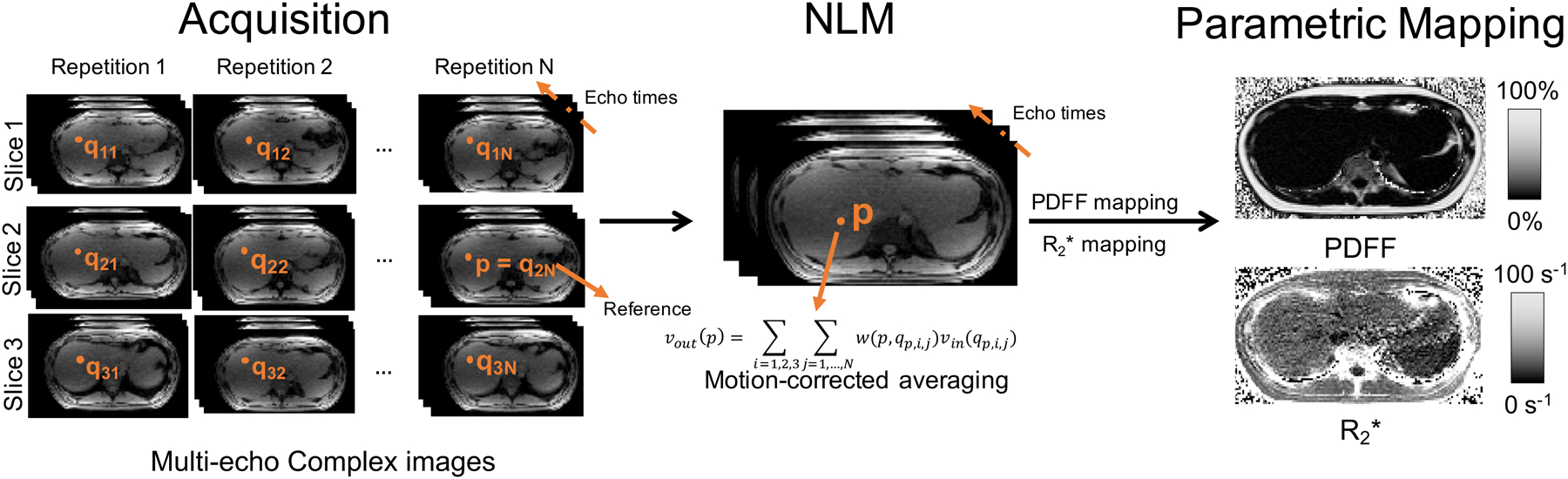
Flow chart of the proposed method for free-breathing CSE imaging, including NLM-based motion corrected averaging. 2D multi-echo slices are acquired sequentially (ie: with a short temporal footprint) with N repetitions obtained during free-breathing. Subsequently, motion-corrected averaging is performed based on NLM in order to obtain high-SNR images with minimal motion artifacts. In this work, the slice window size is 3 (i.e., three consecutive slices are considered for motion-corrected averaging). Multi-echo image pixel values v_out(p) at pixel p of slice 2 are calculated by motion-corrected, weighted averaging of pixels {q_i,j,i ∈ [1, 3], j ∈ [1, N]} arising from the N repetitions and three slices. For motion-correction, pixels are selected from each slice and repetition using a patch-based similarity metric. The weight w(p, q_i,j) is estimated from the similarity between the pixels p and q_i,j. NLM processing is performed jointly for all the echoes, and the resulting high-SNR images are subsequently post-processed to obtain ${\text{R}}_2^{*}$ and PDFF maps.

Study data

Simulations:

A simple 3D model of abdominal motion was generated for simulations. The liver in this model undergoes elastic, non-rigid motion in the axial plane and translation along the S/I direction. Two overlapping ellipsoids are used to represent the liver. The lengths of their two minor axes increase by 8% in the axial plane and 3% along the S/I direction respectively and recover circularly with respiratory motion. A sinusoidal model[35] of respiratory motion was applied:

$$g(t)=A{cos}^{2n}(\pi ft)$$

where t is time in minutes, g(t) (mm) is the respiratory displacement, f (breaths/minute) is the respiratory frequency, A (mm) is the amplitude of motion and n is a parameter determining the asymmetry. The simulated respiratory frequency (f) of 10 breaths/minute and the parameter n of 3 were used.

Simulated acquisition parameters for 2D CSE with 10 repetitions included: FOV = 28 × 28 cm², matrix size = 144 × 144, 7 mm slices, 8 echoes, TE₁/ΔTE = 1.2/1.4 ms, TR = 13 ms, and SNR = 10 chosen to match the observed SNR from in vivo images. The total acquisition time for a single repetition including 22 slices is estimated at around 41 sec as: number of slices × number of phase encoding steps × TR.

Healthy volunteer scans:

In order to perform a preliminary evaluation of the proposed method, a healthy volunteer was scanned after obtaining informed written consent and approval from the local institutional review board (IRB). The volunteer was scanned at 3T (MR750, GE Healthcare, Waukesha, WI) using a 32-channel phased array torso coil (Neocoil, Pewaukee, WI). 2D sequential CSE was acquired during free-breathing with 10 repetitions and the following parameters: flip angle = 3°, FOV = 40 × 30 cm², matrix = 192 × 144, TR = 9.5 ms, TE₁/ΔTE = 1.7/1.2 ms, 8 mm slices, 3 echoes/TR with 2 shots, bandwidth = ±62.5 kHz, 22 slices, total scan time = 4 min. Figure 2 illustrates the sequence design and 2 shots acquired in healthy volunteers. In order to assess the robustness of the proposed method to varying levels of respiratory motion, the 2D sequential CSE acquisition was performed twice: once instructing the volunteer to breathe softly (”easy free-breathing”) and once instructing the volunteer to breathe vigorously (“heavy free-breathing”). Reference PDFF and ${\text{R}}_2^{*}$ quantification was performed using a breath-hold 3D CSE-MRI sequence with a standard protocol[5]: flip angle = 3°, FOV = 40 × 30 × 26 cm³, matrix = 224×160×32, 8 mm slices, TR = 9.5 ms, TE₁/ΔTE = 1.1/0.9 ms, 3 echoes/TR with 2 shots, bandwidth = ±125 kHz, total scan time = 21 sec.

Figure 2.

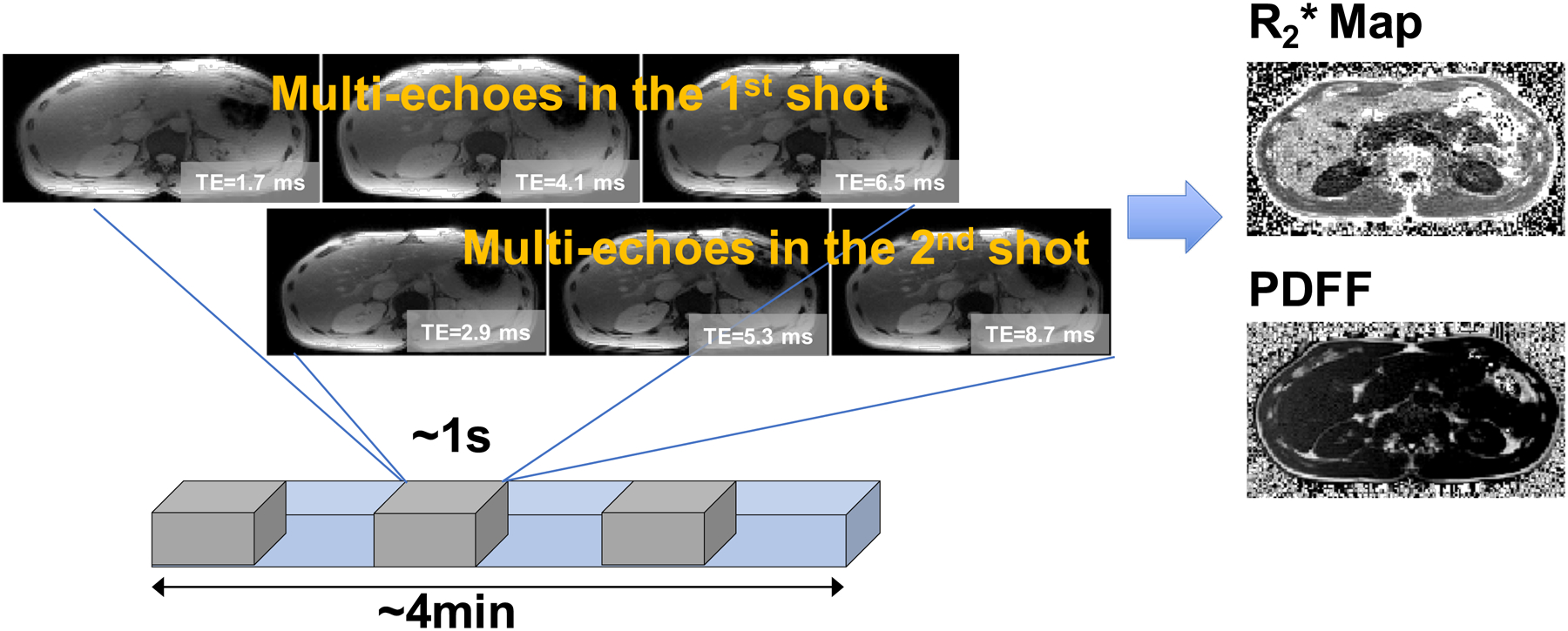
The sequence design and 2 shots acquired in “healthy volunteers” scans. The gray segment represents each repetition. In the overall acquisition (represented by the blue segment), all the repetitions for one slice are acquired consecutively before moving on to the next slice.

Patient scans:

In this IRB-approved study, 30 patients referred for abdominal MRI at our institution were recruited and scanned after informed written consent. For the free breathing scans, patients were instructed to breathe normally. Patient information included 15 male/15 female, age (years): (min-max) 31–82, (mean±standard deviation) 57.8±12.8, weight (kg): 52–136, 91.9±24.9. Height information was recorded for 20 out of the 30 patients, who had a body mass index (kg/m²): 19.1–48.4, 30.8±8.1. Scans were performed at 1.5T (MR750, GE Healthcare, Waukesha, WI) using a 32-channel phased array torso coil (Neocoil, Pewaukee, WI). Four different CSE-MRI acquisitions were performed in each patient: 2D sequential FB with 10 repetitions, 3D BH, 3D Nav and 3D FB. Acquisition parameters for each sequence are described in Table 1.

Table 1.

Imaging protocols in patient studies.

	3D BH	3D FB	3D Nav	2D Sequential FB
Flip angle	5°	5°	5°	5°
FOV	42×42 cm2	42×42 cm2	42×42 cm2	42×42 cm2
Matrix	192×160	192×160	220×176	180×144
Slice thickness	8 mm	8 mm	8 mm	8 mm
TR	14.9 ms	14.9 ms	16.1 ms	12.8 ms
Echo train length	6	6	6	6
TE1	1.1 ms	1.1 ms	1.2 ms	1.3 ms
Δ TE	1.9 ms	1.9 ms	2.1 ms	1.9 ms
Bandwidth	±100 kHz	±100 kHz	±100 kHz	±62.5 kHz
Scan time	21 sec	21 sec	1 min 59 sec	3 min 50 sec

NLM-based motion-corrected averaging

In this study, NLM-based motion-corrected averaging from multiple 2D sequential repetitions was performed jointly for all echo times (Figure 1), in order to maintain all processing consistent across echoes. A reference repetition was picked automatically for each slice, as the repetition with minimal average difference with other repetitions, based on the hypothesis that this approach will select a reference repetition that is free of major artifacts and also close to many other repetitions (to enable effective subsequent averaging). The difference was calculated by the average of root-mean-squared differences between the chosen repetition and the rest of repetitions. Next, NLM motion-corrected averaging was performed[29], as follows: given the pixel located at position p for the current slice in the multi-echo reference images (I_ref), the algorithm finds the most similar pixel in a search window in each of the neighboring slices for each of the repetitions based on neighborhood similarity over a comparison window. Let ${\mathcal{N}}_k$ denote a square region over the comparison window of width L_N centered at pixel k, and ${\mathcal{S}}_k$ denote a square region over the search window of width L_S centered at pixel k. The neighborhood similarity is measured by the Gaussian-weighted Euclidean distance d(p, q_i,j) of the squared neighborhood ${\mathcal{N}}_p$ (centered on p) in the reference images I_ref and the neighborhood ${\mathcal{N}}_{q_{i,j}}$ (centered on q_i,j) in the non-reference images I _i,j:

$$d\left(p,q_{i,j}\right)={\Vert I_{\text{ref}}\left({\mathcal{N}}_p\right)-I_{i,j}\left({\mathcal{N}}_{q,i,j}\right)\Vert }_{2,a}^2,q_{i,j}\in I_{i,j}\left({\mathcal{S}}_p\right)$$ (1)

where I_i,j denotes the measured multi-echo signal located at i-th slice and j-th repetition and ${\mathcal{S}}_p$ is the search window centered at p. Note that the neighborhoods include all acquired echo times, as all echo times are processed jointly in the proposed method to maintain consistency of the CSE data. The parameter a (a = 2 used in this work) denotes the standard deviation (STD) of the Gaussian weighting on L₂ norm of the difference between corresponding pixels, placing larger weights on pixels closer to the center of the square neighborhood. For a pixel p in the reference repetition, the most similar pixel’s position at i-th slice and j-th repetition (as defined by the distance d(p, q_i,j) in Eq.1) is denoted by q_p,i,j, and then pixel values at position q_p,i,j are denoted by v_in(q_p,i,j). Subsequently, the output pixel values v_out(p) at location p for the current slice are calculated as:

$$v_{out}(p)=\sum _{i,j}w\left(p,q_{p,i,j}\right)v_{in}\left(q_{p,i,j}\right),q_{p,i,j}\in I_{i,j}\left({\mathcal{S}}_p\right)$$ (2)

The weight w(p, q_p,i,j) is defined as:

$$w\left(p,q_{p,i,j}\right)=\frac{1}{z}{e}^{-\frac{d\left(p,q_{p,i,j}\right)}{h^2}}$$ (3)

where z is a normalizing factor, namely the sum of exponential items in weights of all the repetitions, $z={\sum }_{i,j}{e}^{-\frac{d\left(p,q_{p,i,j}\right)}{h^2}}$. Finally, h is a filtering parameter which indicates the degree of smoothing, in order to balance motion robustness and SNR.

Impact of NLM Parameters:

Parameters used in NLM method, including the number of adjacent slices, the degree of smoothing (h), the number of repetitions of each slice, the comparison window size (L_N) and the search window size (L_S), are tunable and may affect the image quality and quantitative measurements. In this work, we preliminarily analyzed the impact of different parameter combinations on one slice of images in three patients with low PDFF, moderate PDFF and high PDFF in the Supporting Information S1.1. Additionally, we also preliminarily analyzed the effect of various parameter combinations using the simulation described above, as detailed in the Supporting Information S1.2.

A radiologist (J.S.) with 9 years of experience in MRI evaluated the overall image quality of three subjects reconstructed using different parameter combinations using a 5-point Likert scale: 1, non-diagnostic; 2, severe artifacts, limited diagnostic confidence; 3, modest artifacts, slightly impaired diagnostic confidence; 4, minor artifacts, diagnostic confidence not affected; 5, no significant artifacts, full diagnostic confidence. Moreover, the STDs of liver PDFF and ${\text{R}}_2^{*}$ in 2D CSE-MRI were compared to the STDs of PDFF and ${\text{R}}_2^{*}$ in the reference 3D BH CSE-MRI, respectively. Detailed information is explained again in the Supporting Information S1.

PDFF and ${\text{R}}_2^{*}$ mapping

Parametric fitting from the complex echo images was performed in order to obtain PDFF and ${\text{R}}_2^{*}$ maps from each of the acquisitions described above, as well as for the NLM-processed CSE 2D data. This parametric fitting, which has been described in previous works[36, 37, 38] is based on a two-step algorithm, including: 1) regularized estimation of the B₀ field map imposing spatial smoothness to avoid fat-water swaps[39], followed by 2) voxel-independent non-linear least squares fitting which results in water-only and fat-only images, with correction for ${\text{R}}_2^{*}$ decay[40, 41], spectral complexity of the fat signals[42, 40], and phase errors[36, 41]. A low flip angle was used for the acquisition to minimize T₁ bias [43]. Finally, these water-only and fat-only images were combined at each voxel to generate a PDFF map, including correction for noise bias [43]. This same algorithm also results in fat-corrected ${\text{R}}_2^{*}$ maps.

Data Analysis

To evaluate the performance of different techniques, statistical analysis was performed on the patient studies. One trained analyst drew the regions of interest (ROIs) of all the measurements. This analyst placed a single circular ROI with approximate diameter of 19 mm over each of the nine Couinaud liver segments [44], where the mean and STD of PDFF and ${\text{R}}_2^{*}$ were recorded. The STD over a ROI on a homogeneous tissue region in PDFF or ${\text{R}}_2^{*}$ was used to estimate SNR of various techniques. The ROIs were co-localized in all CSE-MRI images of the same subject. Correlation analysis and Bland-Altman analysis[45] for mean PDFF and ${\text{R}}_2^{*}$ of each segment, were performed to assess correlation and bias between each of the different techniques (3D FB, 3D Nav, 2D 1ave, 2D 10ave and 2D NLM) and the reference (3D BH). In the correlation analysis, Pearson’s correlation coefficient[46] and Lin’s concordance correlation coefficients[47] were calculated. Paired Student’s t-test with Bonferroni correction for STDs of 2D-based reconstructions (2D 1ave, 2D 10ave and 2D NLM) was performed to assess the SNR of different reconstruction techniques from the 2D sequential data. For all statistical tests, the significance threshold was set at p=0.05. All the statistical analysis was performed with MATLAB 2019a (MathWorks, Natick, MA).

One radiologist (J.S.) evaluated the image quality of PDFF and ${\text{R}}_2^{*}$ maps separately using 5-point Likert scale as stated above. The reader was blinded to all image acquisition and reconstruction techniques (i.e., 3D BH, 3D FB, 3D Nav, 2D 1ave, 2D 10ave, 2D NLM) and the reading order of PDFF or ${\text{R}}_2^{*}$ maps in all subjects was randomized. The reader scored on motion artifacts, SNR, image sharpness, and overall impression, separately. The reader also noted other artifacts including signal inhomogeneity or signal loss, etc. Student’s t-test was performed on the reader’s scores for comparison.

Results

Impact of NLM Parameters

In this work, the number of adjacent slices was determined to be three, including the current slice and its two adjacent slices. The maximum liver movement in the slice-encoding (S/I) direction due to the respiratory motion is about 24 mm as shown in previous studies[48]. For this reason, the tissue displacement was assumed to be restricted to three consecutive slices with a slice thickness of 8 mm in 2D CSE-MRI.

The other parameters used in NLM reconstruction were determined based on the scores on image quality by the radiologist, quantitative measurements and additional analysis, and the simulation, as detailed in the Supporting Information S1.1, S1.2 and Supporting Figures S1–S4. NLM searched for similar pixels over a 3-by-3 pixels square window centered at the reference pixel. The neighborhood similarity measure was based on a 11-by-11 pixels neighborhood. The degree of smoothing (h) was chosen at 0.11. Finally, 10 repetitions were used in our experiments.

Simulations

Figure 3 shows representative measurements of ${\text{R}}_2^{*}$ and PDFF in the simulation. 2D NLM (10 rep) resulted in lower ROI-based STDs of liver PDFF (2.7%) and ${\text{R}}_2^{*}$ (8.2 s⁻¹) compared with those of 2D 1ave (PDFF: 8.7%, ${\text{R}}_2^{*}$: 33.2 s⁻¹) and 2D 10ave (PDFF: 3.1%, ${\text{R}}_2^{*}$: 13.6 s⁻¹). Substantial blurring near the tissue interfaces was observed in 2D 10ave, but not in 2D NLM (10 rep). Thus, the simulation of the abdominal motion indicated that 2D NLM (10 rep) improved SNR compared to 2D 1ave, and reduced the blurring compared to 2D 10ave.

Figure 3.

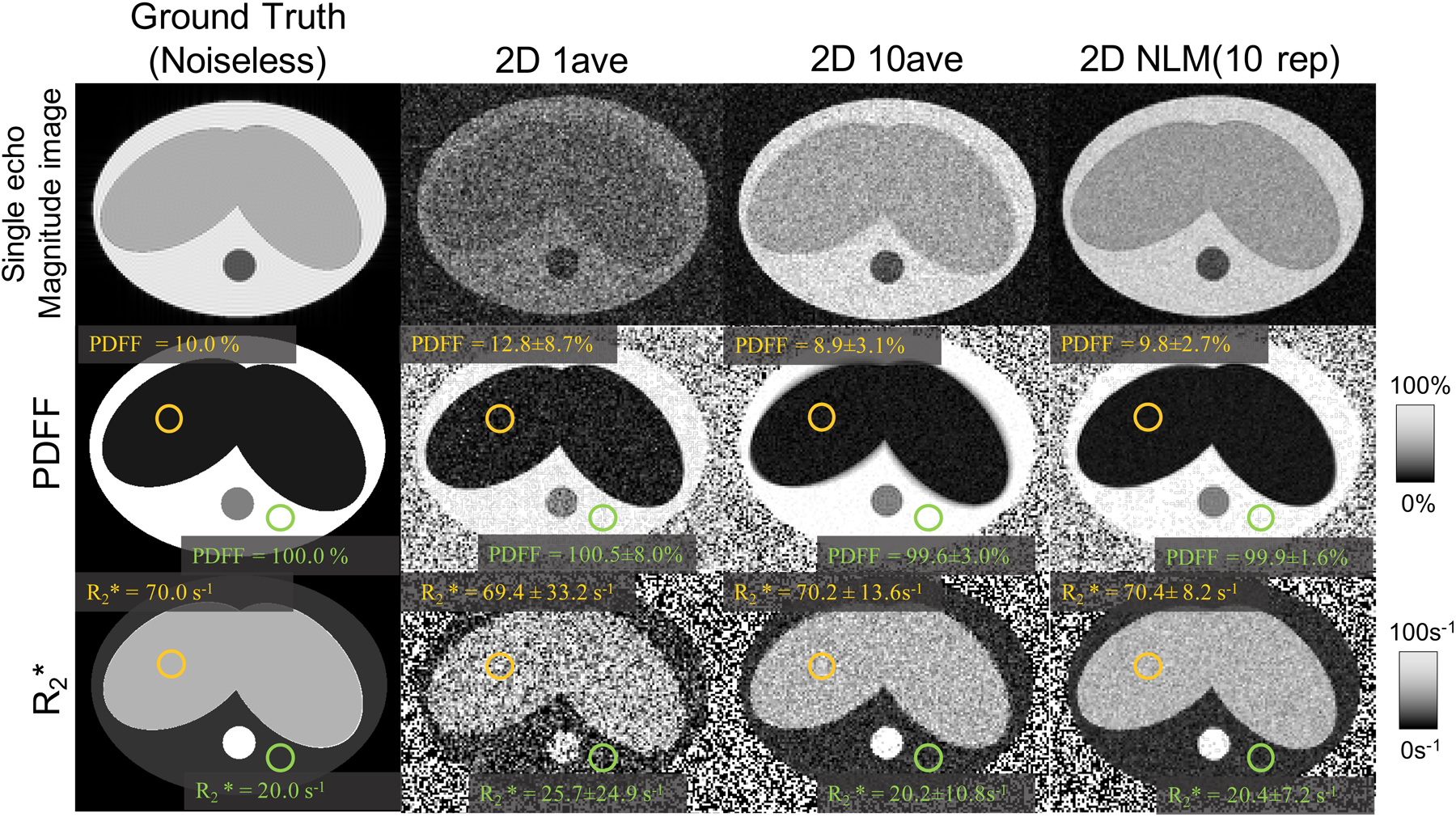
Representative simulation results of a simple abdominal motion model. Noiseless ground truth, single-average (“1ave”) as well as direct averaging (“10ave”) maps are shown for comparison to the proposed NLM method. The results illustrate the potential of the proposed NLM method to provide PDFF and ${\text{R}}_2^{*}$ maps with low bias, high SNR and minimal motion-related blurring and artifacts (compared to direct averaging).

Healthy Volunteer Study

Figure 4 illustrates the results of the in vivo liver 3D BH and 2D CSE data acquired during “easy breathing” and “heavy breathing” from the same healthy volunteer, respectively. In 3D BH, liver PDFF and ${\text{R}}_2^{*}$ of the ROI were −0.8 ± 1.8% and 64.8 ± 7.3 s⁻¹, respectively. In the “easy breathing” acquisition, PDFF of the ROI in 2D 1ave, 2D 10ave and 2D NLM (10 rep) were 0.2 ± 24.4%, 2.8 ± 7.4% and 3.1 ± 8.3%, respectively. ${\text{R}}_2^{*}$ of the ROI in 2D 1ave, 2D 10ave and 2D NLM (10 rep) were 64.4 ± 18.7 s⁻¹, 72.8 ± 9.8 s⁻¹ and 70.1 ± 9.9 s⁻¹, respectively. 2D 10ave and 2D NLM (10 rep) showed comparable PDFF and ${\text{R}}_2^{*}$ measurements, both with lower STDs compared to 2D 1ave. In the “heavy breathing” acquisition, PDFF of the ROI in 2D 1ave, 2D 10ave and 2D NLM (10 rep) were −2.9 ± 26.0%, 6.4 ± 9.1% and 2.5 ± 8.9%, respectively. ${\text{R}}_2^{*}$ measured by these methods were 72.6 ± 18.6 s⁻¹,164.9 ± 13.0 s⁻¹ and 73.3 ± 9.8 s⁻¹, respectively. Importantly, 2D 10ave led to bias in ${\text{R}}_2^{*}$ and PDFF, whereas 2D NLM (10 rep) maintained accurate quantification.

Figure 4.

PDFF and ${\text{R}}_2^{*}$ maps from a volunteer instructed to perform “easy” and “heavy” breathing in separate 2D sequential multi-repetition CSE free-breathing acquisitions. Both direct averaging (2D 10ave) and NLM are able to improve SNR (reduce standard deviations) compared to a single average. However, direct averaging results in noticeable artifacts, particularly under “heavy” breathing conditions, whereas the proposed NLM method results in reproducible PDFF and ${\text{R}}_2^{*}$ measurements regardless of the breathing pattern.

Patient Study

Statistical Analysis.

Figure 5 shows representative PDFF and ${\text{R}}_2^{*}$ maps obtained from two patients with moderate and high liver fat, respectively, using 3D BH, 3D FB, 3D Nav, 2D 1ave, 2D 10ave and 2D NLM (10 rep). Compared to the reference (3D BH), 3D FB and 3D Nav resulted in noticeable motion artifacts. 2D 1ave resulted in no motion artifacts but lower SNR than other techniques: The measured STDs of PDFF were more than 5.5% but the STDs of PDFF from other techniques were from 2.2% to 4.4%. 2D 10ave resulted in improved SNR but biased measurements of ${\text{R}}_2^{*}$: ${\text{R}}_2^{*}$ for two patients with moderate and high liver fat were 74.8±24.1 s⁻¹ and 51.5±7.6 s⁻¹ respectively, higher than ${\text{R}}_2^{*}$ of the reference (moderate fat: 25.1±12.0 s⁻¹, high fat: 34.6±6.4 s⁻¹). 2D NLM (10 rep) resulted in comparable PDFF and ${\text{R}}_2^{*}$ measurements relative to the reference 3D BH, also with comparable SNR.

Figure 5.

PDFF and ${\text{R}}_2^{*}$ measurements of patient scans with moderate and high liver fat using six different techniques: 3D BH, 3D FB, 3D Nav, 2D 1ave and 2D 10ave and 2D NLM (10 rep). Compared to other techniques, the proposed NLM-based method is able to provide high-image quality, high-SNR, and low-bias quantification of PDFF and ${\text{R}}_2^{*}$ during free-breathing, relative to the reference 3D BH acquisitions.

Figure 6 shows a case of focal, mass-like fat deposition. PDFF maps of 2D 10ave and 2D NLM (10 rep) both kept the lesion in the liver as pointed by red arrows. However, 2D 10ave introduced blurring compared to 2D NLM (10 rep), distorting the shape of the lesion compared to that in the post-contrast T_1w map (pointed by the red arrow). In addition, the lesion on pancreas tail pointed by the blue arrow was blurred in 2D 10ave compared to that in 2D 1ave and 2D NLM (10 rep). In summary, this example illustrates that 2D NLM (10 rep) can simultaneously preserve fine details and denoise images.

Figure 6.

Example of images from a clinic study with a fat-containing lesion in the left liver lobe (pointed by the red arrow). As demonstrated in this example, 2D NLM (10 rep) and 2D 10ave are able to accurately depict the lesion, compared to 2D 1ave and 3D BH. However, 2D 10ave results in blurring as pointed by the blue arrow. This example demonstrates the ability of the proposed NLM method in preserving fine structures, even relatively small focal lesions.

Reader Study.

Figure 7(a) plots mean reader scores for the PDFF maps from the 30 subjects. The reader’s score on motion artifacts of all 2D techniques (>4) was higher compared to the score of all 3D techniques (3D BH=3.3, 3D FB=1.8, 3D Nav=2.2, all p<0.0001). The score on SNR was the highest in 3D Nav (=3.4) with p<0.0001 compared to all other techniques, and comparable (~2.5, all p>0.05 between each other) in 3D BH, 3D FB, 2D 10ave, and 2D NLM (10 rep), while it was the lowest in 2D 1ave (=1.3) with p<0.05. The score on image sharpness of all 3D techniques (>3) was higher than the score of all 2D techniques (~2), with p<0.001. The score on overall impression was relatively high in 3D BH, 3D Nav, 2D 10ave, and 2D NLM (10 rep) (>2), compared to that in 3D FB and 2D 1ave (~1.6).

Figure 7.

Top: Mean scores of the reader study on motion artifacts, SNR, image sharpness and overall impression in PDFF (a) and ${\text{R}}_2^{*}$ maps (b) of 3D BH, 3D FB, 3D Nav, 2D 1ave, 2D 10ave, and 2D NLM (10 rep), separately. Bottom: The number of datasets with signal loss or signal inhomogeneity observed in the PDFF (a) and ${\text{R}}_2^{*}$ (b) maps.

Figure 7(b) plots mean scores for the ${\text{R}}_2^{*}$ maps from the 30 subjects. The reader’s score on motion artifacts of all 2D techniques (>3.4) was significantly higher compared to the score of all 3D techniques (3D BH=3.1, 3D FB=1.6, 3D Nav=2.1) with p<0.0001. The score on SNR was also the highest in 3D Nav (=3.3) with p<0.05, and comparable (~2.5, all p>0.05) in 3D BH, 3D FB, 2D 10ave and 2D NLM (10 rep), and it was also the lowest in 2D 1ave (=1.4) with p<0.05 compared to other techniques. The score on image sharpness was the highest in 3D Nav (=3.6) with p<0.0001, and comparable (~2.8, p>0.05 between each other) in 3D BH, 2D 10ave and 2D NLM (10 rep), but relatively low in 3D FB (=2.4) and 2D 1ave (=1.5). The score on overall impression was higher in 3D BH, 3D Nav, 2D 10ave and 2D NLM (10 rep) (~2.4) than in 3D FB and 2D 1ave (~1.5) with p<0.05.

Both 2D NLM (10 rep) and 2D 10ave had relatively high performance on motion-robustness, SNR, and overall impression. However, signal inhomogeneity or signal loss were observed in the PDFF/${\text{R}}_2^{*}$ map of 3 (PDFF) /12 (${\text{R}}_2^{*}$) subjects in 2D 10ave, respectively, versus 3 (PDFF) /1 (${\text{R}}_2^{*}$) subjects in 2D NLM (10 rep). In other methods, signal inhomogeneity or signal loss were observed in the ${\text{R}}_2^{*}$ map of 3 subjects in 3D FB and 6 subjects in 2D 1ave, and in the PDFF map of 1 subject in 3D FB, and 1 subject in 2D 1ave. Figure 7 (bottom) plots the number of subjects with signal inhomogeneity or signal loss observed in the PDFF/${\text{R}}_2^{*}$ maps obtained with all techniques.

Bland-Altman Analysis.

Bias±95 % limits of agreement (LOA) and p-values from Bland-Altman analysis of liver PDFF and ${\text{R}}_2^{*}$ obtained using different techniques (3D FB, 3D Nav, 2D 1ave, 2D NLM (10 rep) and 2D 10ave) compared to the reference (3D BH) for each ROI are reported in the Supporting Table S1. Narrower LOAs of both liver PDFF and ${\text{R}}_2^{*}$ measurements of 2D techniques, especially 2D NLM (10 rep) and 2D 10ave, were observed. Figure 8 showed Bland-Altman plots of PDFF and ${\text{R}}_2^{*}$ of two ROIs in liver segment 5 and 6, separately. 2D NLM (10 rep) resulted in narrower LOAs of both PDFF and ${\text{R}}_2^{*}$, compared with 3D FB, 3D Nav, 2D 1ave. The results of the segment 6 and other segments were consistent.

Figure 8.

Bland-Altman analysis of ${\text{R}}_2^{*}$ and PDFF for different techniques of two ROIs in liver segment 5 and 6 across all patients (using a standard 3D BH CSE technique as the reference), demonstrating low bias and narrow limits of agreement of the proposed NLM technique.

Correlation analysis.

Pearson’s correlation coefficient (Pearson’s r), Lin’s concordance correlation coefficients (ρ_c) and 95% confidence interval of correlation analysis of liver PDFF and ${\text{R}}_2^{*}$ of 2D 1ave, 2D 10ave and 2D NLM (10 rep) are reported in the Supporting Table S2. Correlation analysis on liver PDFF and ${\text{R}}_2^{*}$ measurements showed a higher Pearson’s r (from 0.93 to 1.00) and higher ρ_c (from 0.92 to 0.99) in 2D NLM than that in 3D FB (Pearson’s r: 0.77 to 0.95, ρ_c: 0.72 to 0.95), 3D Nav (Pearson’s r: 0.70 to 0.99, ρ_c: 0.67 to 0.99) or 2D 1ave (Pearson’s r: 0.94 to 0.99, ρ_c: 0.92 to 0.98), when compared to the standard 3D BH. 2D 10ave resulted in relatively low correlation for ${\text{R}}_2^{*}$ quantification (Pearson’s r: 0.74 to 0.97, ρ_c: 0.68 to 0.95), but high correlation for PDFF quantification (Pearson’s r: 0.97 to 1.00, ρ_c: 0.96 to 0.98).

Paired Student’s t-test of STDs of liver PDFF and ${\text{R}}_2^{*}$ of 2D techniques:

Paired Student’s t-test with Bonferroni correction (reported in the Supporting Table S3) of STDs of liver PDFF and ${\text{R}}_2^{*}$ measurements for each ROI showed a significant difference of 2D NLM (10 rep) vs. 2D 1ave and 2D 1ave vs. 2D 10ave (p<0.05). There was no significant difference of STD of measurements between 2D NLM (10 rep) and 2D 10ave. These results are plotted in Figure 9.

Figure 9.

The range of STD of the three 2D techniques in each liver segment in this study including 30 patients. In the PDFF of Segment 1 (top), the STD is in the range of 4 to 12% in 2D 1ave, which was significantly higher (p<0.05, shown in the Supporting Table S3) than the STD of 2 to 6% in both 2D 10ave and 2D NLM (10 rep). Similarly, the STD of PDFF in other segments in 2D 1ave is higher than the STD in 2D 10ave and 2D NLM (10 rep) (p<0.05). The STDs of ${\text{R}}_2^{*}$ in the 9 liver segments are consistently high (p>0.05).

Discussion

This work proposed and evaluated a method for free-breathing 2D sequential CSE based on a multi-repetition acquisition with motion-corrected averaging, for motion-robust mapping of PDFF and ${\text{R}}_2^{*}$ in the liver. By evaluating the performance of the proposed method and other 2D and 3D CSE techniques in both simulations and in vivo scans, we have demonstrated the feasibility of the proposed CSE-NLM method for free-breathing PDFF and ${\text{R}}_2^{*}$ quantification in the abdomen. The proposed 2D CSE-NLM method exhibited fewer motion artifacts than other 3D techniques (3D Nav and 3D FB) and comparable relatively high SNR with 2D 10ave. Furthermore, 2D NLM demonstrated promising performance for the preservation of localized features in the presence of motion.

The proposed NLM-based method for 2D CSE-MRI provides a novel approach for liver fat and iron quantification during free-breathing. This approach may be complementary to existing 3D techniques, including respiratory gating [49] based on bellows and navigators. For instance, the proposed method may be preferable to respiratory gating-based methods in cases of irregular breathing, where the lack of periodicity of the breathing motion may introduce artifacts in methods that assume periodic motion. This potential advantage of the proposed method may be important for widespread dissemination of CSE-MRI for liver fat and iron quantification. Further, this approach may enable a reliable clinical workflow for liver fat and ${\text{R}}_2^{*}$ quantification without the need for breath-holds, which is important in pediatric imaging. Indeed, NAFLD represents a growing concern for children[50], particularly in the context of the current obesity epidemic. Motion robust, free-breathing CSE-MRI acquisitions require a short temporal footprint (e.g.: ~1–2 s). The techniques improved by NLM may make contributions to quantification of liver fat content in this challenging and clinically relevant patient population. Moreover, the proposed NLM-based method motion-corrected averaging framework is not specific to CSE imaging of the liver. Indeed, this approach may be relevant to other quantitative imaging applications beyond CSE, such as diffusion imaging and T₂/T₁ relaxometry, as well as imaging of other abdominal and cardiovascular imaging applications.

This study proposes a motion-corrected averaging method for SNR enhancement from multiple repetitions. As an alternative, a wide variety of denoising filtering methods have been proposed for SNR-enhancement from a single repetition. Gaussian filtering[51] improves SNR but can lead to blurring across edges[29] To preserve image edges, the anisotropic diffusion filter[52, 53, 30] method was proposed, which can protect edges by averaging pixels in the orthogonal direction of the local gradient, however, it may result in a loss of small features[54]. Wavelet-based filters[55, 56] are also widely used for denoising, although they may introduce artifacts in the denoised image[54]. NLM as a post-processing method has been proposed to denoise magnitude MR images[54] which demonstrated its potential to improve SNR while preserving edges. This method enables additional SNR gains in the proposed NLM-based motion-corrected averaging.

There are still several limitations in this study. Comparison with 3D navigated CSE acquisitions in our clinical study was not performed using equal acquisition times of 2D CSE acquisitions due to scan time limitation, and the focus on obtaining sufficient 2D sequential data for this early-stage validation study. However, we have evaluated the impact of TEs and SNR in simulations in the Supporting Information S2, as well as Supporting Figures S5 and S6. The results indicated that 2D NLM was relatively insensitive to the choice of TEs. Different field strengths were used in the healthy volunteer and patient experiments due to practical constraints on our access to scanners. Thus, the differences in performance due to the field strength still need to be evaluated in future work, although we do not expect major differences in performance of the proposed method across field strengths. Further, the selection of NLM parameters was based on the quantitative measurements of PDFF and ${\text{R}}_2^{*}$ of only three patients, in addition to simulations with a simplified abdominal model in our study. Further fine-tuning of NLM parameters in future works may require analyses with a larger in vivo dataset and simulations with a more sophisticated abdominal model. The proposed NLM-based method has lower STDs than 2D 10ave in the structure free area in simulations, likely due to additional averaging of neighboring slices with similar signals. Also, the proposed method implicitly assumes a locally uniform SNR. The search window in the proposed NLM approach has a moderate size so the assumption of homogeneity over the search window is likely reasonable. Nevertheless, incorporation of spatially-varying SNR into the proposed method would be feasible, eg: by relying on the noise standard deviation maps [57]. Finally, we have not performed explicit comparison between our method and registration-based motion-corrected averaging, due to the challenges associated with 3D registration from 2D axial slices [49].

In conclusion, the proposed NLM-based motion-corrected averaging approach has the potential to enable free-breathing CSE-MRI based PDFF and ${\text{R}}_2^{*}$ mapping in the liver, with low bias, high SNR, and minimal motion artifacts. Upon further validation in relevant patient populations (e.g.: in children), this technique may enable improved liver CSE-MRI with important applications in research and in the clinic.

Supplementary Material

Supporting Information

Figure S1. PDFF and ${\text{R}}_2^{*}$ maps for a patient with low liver fat fraction. (a) Degree of smoothing (h)=0.06, 0.11 and 0.16, 10 repetitions, width of comparison window of 11 pixels and width of search window of 3 pixels. (b) 2, 6 and 10 repetitions were processed with h=0.11, width of comparison window of 11 pixels and width of search window of 3 pixels. (c) Changing the width of comparison window to 3 pixels, 7 pixels and 11 pixels with 10 repetitions, the degrees of smoothing (h) of 0.11 and width of search window of 3 pixels. (d) Changing the width of search window to 3 pixels, 7 pixels and 11 pixels with 10 repetitions, degree of smoothing (h) of 0.11 and width of comparison window of 11 pixels. (e) PDFF and ${\text{R}}_2^{*}$ of 3D BH CSE-MRI as reference.

Figure S2. PDFF and ${\text{R}}_2^{*}$ maps for a patient with moderate liver fat fraction. (a) Degree of smoothing (h) = 0.06, 0.11 and 0.16, 10 repetitions, width of comparison window of 11 pixels and width of search window of 3 pixels. (b) 2, 6 and 10 repetitions were processed with h=0.11, width of comparison window of 11 pixels and width of search window of 3 pixels. (c) Changing the width of comparison window to 3 pixels, 7 pixels and 11 pixels with 10 repetitions, h of 0.11 and width of search window of 3 pixels. (d) Changing the width of search window to 3 pixels, 7 pixels and 11 pixels with 10 repetitions, h of 0.11 and width of comparison window of 11 pixels. (e) PDFF and ${\text{R}}_2^{*}$ of 3D BH CSE-MRI as reference.

Figure S3. PDFF and ${\text{R}}_2^{*}$ maps for a patient with high liver fat fraction. (a) Degree of smoothing (h)=0.06, 0.11 and 0.16, 10 repetitions, width of comparison window of 11 pixels and width of search window of 3 pixels. (b) 2, 6 and 10 repetitions were processed with h=0.11, width of comparison window of 11 pixels and width of search window of 3 pixels. (c) Changing the width of comparison window to 3 pixels, 7 pixels and 11 pixels with 10 repetitions, h of 0.11 and width of search window of 3 pixels. (d) Changing the width of search window to 3 pixels, 7 pixels and 11 pixels with 10 repetitions, h of 0.11 and width of comparison window of 11 pixels. (e) PDFF and ${\text{R}}_2^{*}$ of 3D BH CSE-MRI as reference.

Figure S4. Simulation-based bias (top) and root-mean-square error (bottom) in PDFF and ${\text{R}}_2^{*}$ as a function of four algorithm parameters: degree of smoothing, number of repetitions, width of comparison window, and width of search window. The plots display the bias and root-mean-square error as a function of one of the algorithm parameters, while minimizing across the remaining three algorithm parameters.

Figure S5. PDFF and ${\text{R}}_2^{*}$ maps in three 2D CSE-MRI techniques using different TEs (as acquired using 3D BH, 3D Nav and 2D CSE, respectively, in the in vivo studies). The ground truth values of ${\text{R}}_2^{*}$ and PDFF in the ROI are 10% and 70 s⁻¹, respectively. The standard deviations of PDFF and R2* in the placed ROI vary with TE/ΔTE. 2D 1ave is more sensitive to different TEs, while 2D 10ave and 2D NLM are less sensitive to different TEs.

Figure S6. PDFF and ${\text{R}}_2^{*}$ maps in three 2D CSE-MRI techniques at a SNR of 5, 10, 15 and 20, respectively. The ground truth values of ${\text{R}}_2^{*}$ and PDFF in the ROI are 10% and 70 s⁻¹. The standard deviation of PDFF and ${\text{R}}_2^{*}$ decreases as SNR increases. At a fixed SNR, the standard deviation of PDFF and ${\text{R}}_2^{*}$ is lowest in 2D NLM, and highest in 2D 1ave.

Table S1. Bland-Altman Analysis for different techniques vs. 3D breath-hold CSE (3D BH).

Table S2. Pearson correlation coefficients (r), Lin’s concordance correlation coefficients (ρ_c) and the confidence interval.

Table S3. The p-values of Paired student’s t-test for multi-comparison of 2D techniques.

References

- [1].Bellentani S The epidemiology of non-alcoholic fatty liver disease. Liver international 2017; 37:81–84. [DOI] [PubMed] [Google Scholar]
- [2].Younossi ZM, Koenig AB, Abdelatif D, Fazel Y, Henry L, Wymer M. Global epidemiology of nonalcoholic fatty liver disease—meta-analytic assessment of prevalence, incidence, and outcomes. Hepatology 2016; 64:73–84. [DOI] [PubMed] [Google Scholar]
- [3].Ahmed A, Wong RJ, Harrison SA. Nonalcoholic fatty liver disease review: diagnosis, treatment, and outcomes. Clinical Gastroenterology and Hepatology 2015; 13:2062–2070. [DOI] [PubMed] [Google Scholar]
- [4].RomeroGόmez M, ZelberSagi S, Trenell M. Treatment of NAFLD with diet, physical activity and exercise. Journal of hepatology 2017; 67:829–846. [DOI] [PubMed] [Google Scholar]
- [5].Reeder SB, Sirlin CB. Quantification of liver fat with Magnetic Resonance Imaging. Magnetic Resonance Imaging Clinics 2010; 18:337–357. [DOI] [PMC free article] [PubMed] [Google Scholar]
- [6].Meisamy S, Hines CD, Hamilton G, Sirlin CB, McKenzie CA, Yu H, Brittain JH, Reeder SB. Quantification of hepatic steatosis with T1-independent, -corrected MR imaging with spectral modeling of fat: blinded comparison with MR spectroscopy. Radiology 2011; 258:767–775. [DOI] [PMC free article] [PubMed] [Google Scholar]
- [7].Reeder SB, Hu HH, Sirlin CB. Proton density fat-fraction: a standardized MR-based biomarker of tissue fat concentration. Journal of magnetic resonance imaging 2012; 36:1011–1014. [DOI] [PMC free article] [PubMed] [Google Scholar]
- [8].Idilman IS, Aniktar H, Idilman R, Kabacam G, Savas B, Elhan A, Celik A, Bahar K, Karcaaltincaba M. Hepatic steatosis: quantification by proton density fat fraction with MR imaging versus liver biopsy. Radiology 2013; 267:767–775. [DOI] [PubMed] [Google Scholar]
- [9].Kim KY, Song JS, Kannengiesser S, Han YM. Hepatic fat quantification using the proton density fat fraction (pdff): utility of free-drawn-pdff with a large coverage area. La radiologia medica 2015; 120:1083–1093. [DOI] [PubMed] [Google Scholar]
- [10].Wood JC, Enriquez C, Ghugre N, Tyzka JM, Carson S, Nelson MD, Coates TD. MRI R2 and mapping accurately estimates hepatic iron concentration in transfusion-dependent thalassemia and sickle cell disease patients. Blood 2005; 106:1460–1465. [DOI] [PMC free article] [PubMed] [Google Scholar]
- [11].Vasanawala SS, Yu H, Shimakawa A, Jeng M, Brittain JH. Estimation of liver in transfusion-related iron overload in patients with weighted least squares IDEAL. Magnetic resonance in medicine 2012; 67:183–190. [DOI] [PubMed] [Google Scholar]
- [12].Hernando D, Levin YS, Sirlin CB, Reeder SB. Quantification of liver iron with MRI: state of the art and remaining challenges. Journal of Magnetic Resonance Imaging 2014; 40:1003–1021. [DOI] [PMC free article] [PubMed] [Google Scholar]
- [13].Yokoo T, Shiehmorteza M, Hamilton G, Wolfson T, Schroeder ME, Middleton MS, Bydder M, Gamst AC, Kono Y, Kuo A et al. Estimation of hepatic proton-density fat fraction by using MR imaging at 3.0 T. Radiology 2011; 258:749–759. [DOI] [PMC free article] [PubMed] [Google Scholar]
- [14].Yokoo T, Serai SD, Pirasteh A, Bashir MR, Hamilton G, Hernando D, Hu HH, Hetterich H, Kühn JP, Kukuk GM et al. Linearity, bias, and precision of hepatic proton density fat fraction measurements by using MR imaging: a meta-analysis. Radiology 2017; 286:486–498. [DOI] [PMC free article] [PubMed] [Google Scholar]
- [15].Motosugi U, Hernando D, Bannas P, Holmes JH, Wang K, Shimakawa A, Iwadate Y, Taviani V, Rehm JL, Reeder SB. Quantification of liver fat with respiratory-gated quantitative chemical shift encoded MRI. Journal of Magnetic Resonance Imaging 2015; 42:1241–1248. [DOI] [PMC free article] [PubMed] [Google Scholar]
- [16].Armstrong T, Dregely I, Stemmer A, Han F, Natsuaki Y, Sung K, Wu HH. Free-breathing liver fat quantification using a multiecho 3D stack-of-radial technique. Magnetic resonance in medicine 2018; 79:370–382. [DOI] [PMC free article] [PubMed] [Google Scholar]
- [17].Pooler BD, Hernando D, Ruby JA, Ishii H, Shimakawa A, Reeder SB. Validation of a motion-robust 2D sequential technique for quantification of hepatic proton density fat fraction during free breathing. Journal of Magnetic Resonance Imaging 2018; 48:1578–1585. [DOI] [PMC free article] [PubMed] [Google Scholar]
- [18].Yokoo T, Bydder M, Hamilton G, Middleton MS, Gamst AC, Wolfson T, Hassanein T, Patton HM, Lavine JE, Schwimmer JB et al. Nonalcoholic fatty liver disease: diagnostic and fat-grading accuracy of low-flip-angle multiecho gradient-recalled-echo MR imaging at 1.5T. Radiology 2009; 251:67–76. [DOI] [PMC free article] [PubMed] [Google Scholar]
- [19].Anand CS, Sahambi JS. Wavelet domain non-linear filtering for MRI denoising. Magnetic Resonance Imaging 2010; 28:842–861. [DOI] [PubMed] [Google Scholar]
- [20].Mohan J, Krishnaveni V, Guo Y. A survey on the magnetic resonance image denoising methods. Biomedical signal processing and control 2014; 9:56–69. [Google Scholar]
- [21].Sharif M, Hussain A, Jaffar MA, Choi TS. Fuzzy-based hybrid filter for rician noise removal. Signal, Image and Video Processing 2016; 10:215–224. [Google Scholar]
- [22].Ali HM. MRI medical image denoising by fundamental filters in “High-Resolution Neuroimaging-Basic Physical Principles and Clinical Applications”, pp. 111–124. InTech, 2018. [Google Scholar]
- [23].Rajan J, Veraart J, VanAudekerke J, Verhoye M, Sijbers J. Nonlocal maximum likelihood estimation method for denoising multiple-coil magnetic resonance images. Magnetic Resonance Imaging 2012; 30:1512–1518. [DOI] [PubMed] [Google Scholar]
- [24].Lam F, Babacan SD, Haldar JP, Weiner MW, Schuff N, Liang ZP. Denoising diffusion-weighted magnitude MR images using rank and edge constraints. Magnetic Resonance in Medicine 2014; 71:1272–1284. [DOI] [PMC free article] [PubMed] [Google Scholar]
- [25].Lugauer F, Nickel D, Wetzl J, Kannengiesser SA, Maier A, Hornegger J. Robust spectral denoising for water-fat separation in Magnetic Resonance Imaging. In: International Conference on Medical Image Computing and Computer-Assisted Intervention, 2015. pp. 667–674. [Google Scholar]
- [26].Gal Y, Mehnert AJ, Bradley AP, McMahon K, Kennedy D, Crozier S. Denoising of dynamic contrast-enhanced MR images using dynamic nonlocal means. IEEE transactions on medical imaging 2009; 29:302–310. [DOI] [PubMed] [Google Scholar]
- [27].Tryggestad E, Flammang A, HanOh S, Hales R, Herman J, McNutt T, Roland T, Shea SM, Wong J. Respiration-based sorting of dynamic MRI to derive representative 4D-MRI for radiotherapy planning. Medical physics 2013; 40:051909. [DOI] [PubMed] [Google Scholar]
- [28].Kochunov P, Lancaster JL, Glahn DC, Purdy D, Laird AR, Gao F, Fox P. Retrospective motion correction protocol for high-resolution anatomical MRI. Human brain mapping 2006; 27:957–962. [DOI] [PMC free article] [PubMed] [Google Scholar]
- [29].Buades A, Coll B, Morel JM. A non-local algorithm for image denoising. In: Computer Vision and Pattern Recognition, 2005. CVPR 2005. IEEE Computer Society Conference on, 2005. pp. 60–65. [Google Scholar]
- [30].Samsonov AA, Johnson CR. Noise-adaptive nonlinear diffusion filtering of MR images with spatially varying noise levels. Magnetic Resonance in Medicine 2004; 52:798–806. [DOI] [PubMed] [Google Scholar]
- [31].Manjόn JV, Coupé P, MartíBonmatí L, Collins DL, Robles M. Adaptive non-local means denoising of MR images with spatially varying noise levels. Journal of Magnetic Resonance Imaging 2010; 31:192–203. [DOI] [PubMed] [Google Scholar]
- [32].Crawley AP, Wood ML, Henkelman RM. Elimination of transverse coherences in flash MRI. Magnetic resonance in medicine 1988; 8:248–260. [DOI] [PubMed] [Google Scholar]
- [33].Hernando D, Kramer JH, Reeder SB. Multipeak fat-corrected complex relaxometry: theory, optimization, and clinical validation. Magnetic resonance in medicine 2013; 70:1319–1331. [DOI] [PMC free article] [PubMed] [Google Scholar]
- [34].Asbach P, Warmuth C, Stemmer A, Rief M, Huppertz A, Hamm B, Taupitz M, Klessen C. High spatial resolution T1-weighted MR imaging of liver and biliary tract during uptake phase of a hepatocyte-specific contrast medium. Investigative radiology 2008; 43:809–815. [DOI] [PubMed] [Google Scholar]
- [35].Lujan AE, Balter JM, TenHaken RK. A method for incorporating organ motion due to breathing into 3D dose calculations in the liver: sensitivity to variations in motion. Medical physics 2003; 30:2643–2649. [DOI] [PubMed] [Google Scholar]
- [36].Hernando D, Liang ZP, Kellman P. Chemical shift–based water/fat separation: A comparison of signal models. Magnetic resonance in medicine 2010; 64:811–822. [DOI] [PMC free article] [PubMed] [Google Scholar]
- [37].Yu H, Shimakawa A, Hines CD, McKenzie CA, Hamilton G, Sirlin CB, Brittain JH, Reeder SB. Combination of complex-based and magnitude-based multiecho water-fat separation for accurate quantification of fat-fraction. Magnetic resonance in medicine 2011; 66:199–206. [DOI] [PMC free article] [PubMed] [Google Scholar]
- [38].Hernando D, Sharma SD, AliyariGhasabeh M, Alvis BD, Arora SS, Hamilton G, Pan L, Shaffer JM, Sofue K, Szeverenyi NM et al. Multisite, multivendor validation of the accuracy and reproducibility of proton-density fat-fraction quantification at 1.5T and 3T using a fat–water phantom. Magnetic resonance in medicine 2017; 77:1516–1524. [DOI] [PMC free article] [PubMed] [Google Scholar]
- [39].Hernando D, Kellman P, Haldar J, Liang ZP. Robust water/fat separation in the presence of large field inhomogeneities using a graph cut algorithm. Magnetic Resonance in Medicine 2010; 63:79–90. [DOI] [PMC free article] [PubMed] [Google Scholar]
- [40].Yu H, Shimakawa A, McKenzie CA, Brodsky E, Brittain JH, Reeder SB. Multiecho water-fat separation and simultaneous estimation with multifrequency fat spectrum modeling. Magnetic Resonance in Medicine 2008; 60:1122–1134. [DOI] [PMC free article] [PubMed] [Google Scholar]
- [41].Hamilton G, Yokoo T, Bydder M, Cruite I, Schroeder ME, Sirlin CB, Middleton MS. In vivo characterization of the liver fat 1h MR spectrum. NMR in biomedicine 2011; 24:784–790. [DOI] [PMC free article] [PubMed] [Google Scholar]
- [42].Bydder M, Yokoo T, Hamilton G, Middleton MS, Chavez AD, Schwimmer JB, Lavine JE, Sirlin CB. Relaxation effects in the quantification of fat using gradient echo imaging. Magnetic resonance imaging 2008; 26:347–359. [DOI] [PMC free article] [PubMed] [Google Scholar]
- [43].Liu CY, McKenzie CA, Yu H, Brittain JH, Reeder SB. Fat quantification with ideal gradient echo imaging: correction of bias from T1 and noise. Magnetic Resonance in Medicine 2007; 58:354–364. [DOI] [PubMed] [Google Scholar]
- [44].Campo CA, Hernando D, Schubert T, Bookwalter CA, Pay AJV, Reeder SB. Standardized approach for ROI-based measurements of proton density fat fraction and in the liver. American Journal of Roentgenology 2017; 209:592–603. [DOI] [PMC free article] [PubMed] [Google Scholar]
- [45].Doğan NÖ. Bland-altman analysis: A paradigm to understand correlation and agreement. Turkish journal of emergency medicine 2018; 18:139–141. [DOI] [PMC free article] [PubMed] [Google Scholar]
- [46].Sedgwick P Pearson’s correlation coefficient. Bmj 2012; 345:e4483. [Google Scholar]
- [47].Lawrence I, Lin K. A concordance correlation coefficient to evaluate reproducibility. Biometrics 1989; pp. 255–268. [PubMed] [Google Scholar]
- [48].Bussels B, Goethals L, Feron M, Bielen D, Dymarkowski S, Suetens P, Haustermans K. Respiration-induced movement of the upper abdominal organs: a pitfall for the three-dimensional conformal radiation treatment of pancreatic cancer. Radiotherapy and Oncology 2003; 68:69–74. [DOI] [PubMed] [Google Scholar]
- [49].Kellman P, Chefd’hotel C, Lorenz CH, Mancini C, Arai AE, McVeigh ER. Fully automatic, retrospective enhancement of real-time acquired cardiac cine MR images using image-based navigators and respiratory motion-corrected averaging. Magnetic Resonance in Medicine 2008; 59:771–778. [DOI] [PubMed] [Google Scholar]
- [50].Rehm JL, Wolfgram PM, Hernando D, Eickhoff JC, Allen DB, Reeder SB. Proton density fat-fraction is an accurate biomarker of hepatic steatosis in adolescent girls and young women. European radiology 2015; 25:2921–2930. [DOI] [PMC free article] [PubMed] [Google Scholar]
- [51].Ashburner J, Friston KJ. Voxel-based morphometry—the methods. Neuroimage 2000; 11:805–821. [DOI] [PubMed] [Google Scholar]
- [52].Perona P, Malik J. Scale-space and edge detection using anisotropic diffusion. IEEE Transactions on pattern analysis and machine intelligence 1990; 12:629–639. [Google Scholar]
- [53].Gerig G, Kubler O, Kikinis R, Jolesz FA. Nonlinear anisotropic filtering of MRI data. IEEE Transactions on medical imaging 1992; 11:221–232. [DOI] [PubMed] [Google Scholar]
- [54].Manjón JV, CarbonellCaballero J, Lull JJ, GarcíaMartí G, MartíBonmatí L, Robles M. MRI denoising using non-local means. Medical image analysis 2008; 12:514–523. [DOI] [PubMed] [Google Scholar]
- [55].Nowak RD. Wavelet-based rician noise removal for Magnetic Resonance Imaging. IEEE Transactions on Image Processing 1999; 8:1408–1419. [DOI] [PubMed] [Google Scholar]
- [56].Pizurica A, Philips W, Lemahieu I, Acheroy M. A versatile wavelet domain noise filtration technique for medical imaging. IEEE Trans. Med. Imaging 2003; 22:323–331. [DOI] [PubMed] [Google Scholar]
- [57].Rabanillo I, AjaFernández S, AlberolaLópez C, Hernando D. Exact calculation of noise maps and g-factor in GRAPPA using a k-space analysis. IEEE transactions on medical imaging 2017; 37:480–490. [DOI] [PubMed] [Google Scholar]
Associated Data
This section collects any data citations, data availability statements, or supplementary materials included in this article.
Supplementary Materials
Figure S1. PDFF and maps for a patient with low liver fat fraction. (a) Degree of smoothing (h)=0.06, 0.11 and 0.16, 10 repetitions, width of comparison window of 11 pixels and width of search window of 3 pixels. (b) 2, 6 and 10 repetitions were processed with h=0.11, width of comparison window of 11 pixels and width of search window of 3 pixels. (c) Changing the width of comparison window to 3 pixels, 7 pixels and 11 pixels with 10 repetitions, the degrees of smoothing (h) of 0.11 and width of search window of 3 pixels. (d) Changing the width of search window to 3 pixels, 7 pixels and 11 pixels with 10 repetitions, degree of smoothing (h) of 0.11 and width of comparison window of 11 pixels. (e) PDFF and of 3D BH CSE-MRI as reference.
Figure S2. PDFF and maps for a patient with moderate liver fat fraction. (a) Degree of smoothing (h) = 0.06, 0.11 and 0.16, 10 repetitions, width of comparison window of 11 pixels and width of search window of 3 pixels. (b) 2, 6 and 10 repetitions were processed with h=0.11, width of comparison window of 11 pixels and width of search window of 3 pixels. (c) Changing the width of comparison window to 3 pixels, 7 pixels and 11 pixels with 10 repetitions, h of 0.11 and width of search window of 3 pixels. (d) Changing the width of search window to 3 pixels, 7 pixels and 11 pixels with 10 repetitions, h of 0.11 and width of comparison window of 11 pixels. (e) PDFF and of 3D BH CSE-MRI as reference.
Figure S3. PDFF and maps for a patient with high liver fat fraction. (a) Degree of smoothing (h)=0.06, 0.11 and 0.16, 10 repetitions, width of comparison window of 11 pixels and width of search window of 3 pixels. (b) 2, 6 and 10 repetitions were processed with h=0.11, width of comparison window of 11 pixels and width of search window of 3 pixels. (c) Changing the width of comparison window to 3 pixels, 7 pixels and 11 pixels with 10 repetitions, h of 0.11 and width of search window of 3 pixels. (d) Changing the width of search window to 3 pixels, 7 pixels and 11 pixels with 10 repetitions, h of 0.11 and width of comparison window of 11 pixels. (e) PDFF and of 3D BH CSE-MRI as reference.