

Abstract
High-frequency ventilation is a type of mechanical ventilation therapy applied on patients with damaged or delicate lungs. However, the transport of oxygen down, and carbon dioxide up, the airway is governed by subtle transport processes which hitherto have been difficult to quantify. We investigate one of these mechanisms in detail, nonlinear mean streaming, and the impact of the onset of turbulence on this streaming, via direct numerical simulations of a model 1:2 bifurcating pipe. This geometry is investigated as a minimal unit of the fractal structure of the airway. We first quantify the amount of gas recirculated via mean streaming by measuring the recirculating flux in both the upper and lower branches of the bifurcation. For conditions modeling the trachea-to-bronchi bifurcation of an infant, we find the recirculating flux is of the order of 3–5% of the peak flux . We also show that for conditions modeling the upper generations, the mean recirculation regions extend a significant distance away from the bifurcation, certainly far enough to recirculate gas between generations. We show that this mean streaming flow is driven by the formation of longitudinal vortices in the flow leaving the bifurcation. Second, we show that conditional turbulence arises in the upper generations of the airway. This turbulence appears only in the flow leaving the bifurcation, and at a point in the cycle centered around the maximum instantaneous flow rate. We hypothesize that its appearance is due to an instability of the longitudinal-vortices structure.
Keywords: High-frequency ventilation, Nonlinear mean streaming, Turbulence, Direct numerical simulations
Introduction
Ventilatory support is often required for patients in the intensive care unit and is achieved in the form of mechanical ventilation techniques. The conventional approach to mechanical ventilation is based on the hypothesis that the tidal volume per inflation should exceed the dead space of the airway to facilitate adequate alveolar ventilation; thus, the tidal volume used in conventional mechanical ventilation (CMV) is approximately 75–150% of the patient’s natural respiratory volume [36]. However, such large tidal volumes can cause over distention of lung tissues (barotrauma) and injuries associated with cyclic opening and closing of alveolar tissues (volutrauma). As a remedial alternative to CMV, high-frequency ventilation (HFV) adopts very fast, shallow inflations that are much smaller in volume than the volume of the airway. These small volumes result in small intralung peak pressures and thereby provide a way to protect delicate lungs from over-distention and pressure-induced lung injury, while still providing adequate gas exchange. In contrast to cyclic opening and closing of alveolar units in CMV, HFV uses an adequate mean airway pressure to keep alveoli open during the gas exchange process [17].
These small tidal volumes present an interesting question from a fluid mechanics point of view—if the airway is not emptied and refilled each inflation cycle, how is gas transported throughout the airway? At least six mechanisms are purported to play some role in the gas transport throughout the airway [8, 46]—these being molecular diffusion, Pendelluft effect, cardiogenic mixing, turbulent diffusion, Taylor dispersion, and asymmetric velocity profiles or nonlinear mean streaming. The last three of these appear to be the most likely to dominate and they are the mechanisms which can be controlled via the input pressure waveform. Despite this list of mechanisms, little advance has been made in using knowledge of them to be able to quantify or predict the gas transport that will occur. Protocols for the clinical use of HFV, where they exist, have often been derived with minimal evidence [32, 34, 41, 45].
This has led to a situation where HFV is routinely used in neonatal ICU (NICU), but not in the adult population, as it appears that there are scaling effects that are not understood in the clinic. This is despite a number of experimental and numerical studies of the underlying flows involved. Here, we concentrate our efforts on quantifying the effect of nonlinear mean streaming and the appearance of turbulence in the airflow pertaining to clinically relevant parameters for the application of HFV.
A large number of oscillatory flow studies have been carried out experimentally [37] and numerically [15] in simple bronchial bifurcation models at conditions relevant to HFV.
The oscillatory flow in a single bifurcation model was experimentally studied by Jan et al. [29]. Based on an order of magnitude analysis, this study proposed a benchmark regime classification for respiratory patterns ranging from quiet breathing to HFV. This classification is proposed in the parameter space, where is the average axial displacement of a fluid particle, a is the airway radius and is the Womersley number (). Three major zones, the unsteady (zone I), viscous (zone II) and convective (zone III), were identified in this space depending on the relative dominance of the convective acceleration terms or the viscous terms in the momentum transport equation. The convective zone is further divided into two subcategories (zone IIIa, zone IIIb) based on the experimental evidence. These two subdivisions correspond to the dominating convective acceleration term over the sub-dominant viscous term and the dominating convective acceleration term over the unsteady acceleration term, respectively. Further, there is a turbulent region in the convective zone corresponding to high values of both and .
We used this regime classification to obtain a preliminary understanding of the flow pertaining to existing clinical conditions of HFV. Figure 1 shows the position corresponding to the airflow of each generation in the parameter space where for the first 10 generations of the neonatal airway subjected to HFV, on the map of different regimes based on the scaling analysis from Jan et al. [29] (the calculation of the parameter pairs for each generation is further explained in Sect. 2.4). The uppermost generation is in the zone IIIb and predicted to be susceptible to the appearance of turbulence due to high dimensionless amplitude and frequency of the flow. The subsequent generations lie in the zone IIIa where convective acceleration terms dominate over the viscous term. At the lowest generation cases tested, modeling generations further down the airway, the flow becomes viscous dominated. Since the flows in the upper generations (at least the first 10) are in the convective region, there is the potential for mean streaming to occur due to the dominance of the nonlinear convective terms which can induce a mean flow correction.
Fig. 1.
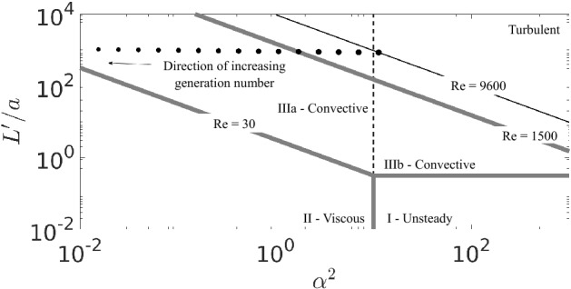
Estimated conditions of the first 10 generations of the neonatal airway subjected to HFV (), superposed on the flow regime diagram proposed by Jan et al. [29]
Nonlinear mean streaming or steady streaming [42] is the net velocity experienced at a given location in a purely oscillating flow due to the difference in velocity fields formed when the flow moves in the forward and backward directions. Such dissimilar velocity fields are caused by nonlinearity which destroys the reversibility. In the bifurcation, this nonlinearity can be introduced either by a curved flow path or varying cross sectional area along the streamwise direction. This phenomenon dictates that while the mean mass flux through a given cross section must be zero (the same amount of mass goes forward and backward across the cross section in one cycle) the flow moves on average in one direction along the core of the flow section and in the opposite direction in the near wall region. Such a flow sets up a direct recirculation that could greatly enhance the gas transport. Haselton and Scherer [21] interpreted the balanced mean flux as a convective-exchange of fluid elements and proposed a coefficient to quantify this process across any arbitrary plane. The same effect was analytically shown by Grotberg [19], through an analysis of oscillatory flow in a diverging channel. Due to the tapered geometry of a diverging channel, the velocity profile along one direction does not remain symmetric with that of the opposite direction. This phenomena holds true for a bifurcating geometry and it has been demonstrated experimentally for tapered channels and conical tubes [7, 16].
The mean streaming velocity fields were extensively reported and analyse in the recent study from Jalal et al. [28], using magnetic resonance velocimetry (MRV) to compare the streamwise and transverse velocity fields in a steady and oscillatory flow in a double bifurcation model. They studied the degree of streamwise velocity variation within a particular cross section of interest using a momentum distortion parameter. Further, they computed iso-surfaces of a scalar quantity used as a vortex identifier and visualized them to provide important insights about the flow development. Interestingly, Jalal et al. [28] suggested that the steady streaming is not the primary gas transport mechanism responsible for HFV.
Defining a secondary flow as the motion of fluid on a perpendicular plane to the streamwise direction, it can be considered as a proxy for the mean streaming phenomenon. The generation of secondary flow is likely to coincide with mean streaming due to the generation of asymmetry. A number of studies have reported the evolution of a transverse velocity field as an important feature influencing the gas mixing [40, 44]. In the Horsfield model for the human bronchial tree [26], consisting of an asymmetric bifurcation in which the left primary bronchus divides into three branches while the right primary bronchus divides into four branches, Tanaka et al. [47] used LDV to verify the effect of secondary flow during oscillatory flow. This study reported that the spatial variation of secondary flow was well correlated with the measured gas transport rates. In addition to these secondary flow features, Heraty et al. [22] and Choi et al. [9] reported the coaxial counterflow feature using stretch rate analysis.
Due to the fact that the mean streaming is a function of the difference between the flow moving backwards and forwards, it may be expected that the generation of turbulence over a portion of the cycle will have some impact on it. The reciprocating flow, even in a straight pipe, can be turbulent during some or all of the reciprocation period [1, 25]. The scales associated with this study are typical to a full-term neonate subjected to high-frequency ventilation: volume per inflation per unit body weight of the infant 1–3 ml/kg and the frequency of therapy in the range of 8–12 Hz. The typical diameter of the endotracheal tube employed is 3 mm. Assuming typical numbers of a body mass of 3 kg, a ventilator frequency of 12 Hz and a sinusoidal variation of the volumetric flow rate over the inflation cycle results in a maximum volumetric flow rate of . These numbers results in and in the trachea and and in the main bronchi of the airway. Consideration of the size of the trachea and the bronchi in the early generations in the airway, and the typical flow rates used during HFV [8], indicates that these flows can be turbulent. This turbulence is also likely to be triggered by the ribbed structure of the tracheal wall providing a flow disturbance at the pipe wall [50]. Due to the presence of sharp curvatures, the ribbed structures may potentially generate streaming fields that are non-trivial in the above scales of gas transport [5, 38]. The presence of such ribbings in the upper airway might cause potential mechanisms of the gas transport in the HFV; however is beyond the scope of this study. Therefore, the ribbings and elasticity of the walls are not taken into consideration in this study.
Peattie and Schwarz [39] studied purely oscillatory flow through a symmetrically branching model of a bronchial bifurcation. They used pulsed hydrogen bubbles for qualitative visualization and frequency-shifted LDV to take quantitative velocity measurements of the flow. They studied the evolution of the instantaneous velocity field along with the transverse velocity fields which were reported to be negligible at all times. During the expiration cycle, for in the mother branch (where the mother branch is the large single pipe), they observed a burst of rapid fluctuations at a frequency between 10 and 100 times the flow frequency, superposed on its fundamental variation. Notably, these rapid velocity fluctuations were never observed in the higher frequency flows, which remained laminar at all times. Rapid velocity fluctuations were never observed at any location in the daughter branches (the smaller pair of pipes). This study did not report the stroke length of the oscillations directly and it is therefore difficult to ascertain how applicable these results are to HFV. However, it does clearly demonstrate that turbulence can be generated for different epochs of time and at different locations during the oscillatory flow in the bifurcation.
In this study, we investigate the nonlinear mean streaming and the onset of turbulence. We employ direct numerical simulations on the basic self-similar unit (1:2 bifurcation) of the fractal structure of the airway. The geometry employed—a single bifurcation consisting of rigid walls—is obviously highly idealised compared to the real airway, with no consideration of vessel compliance or any viscoelastic effects due to mucus layers or cilia. However, this is not as large an approximation from a physiological perspective as might initially be thought, as the upper airway is reasonably stiff (the trachea is cartilage-reinforced), the high mean pressures of HFV further reduce compliance, and cilia layers can be completely sheared away during mechanical ventilation. From a flow perspective, these rigid-vessel simulations can also be directly compared to the recent experimental characterisations of Jalal et al. [28]. We have also deliberately removed the coupling between the generations, to focus on the flow phenomena generated in a single bifurcation without the impact of variable inlet and outlet conditions. A series of generations of the airway are modeled by varying the amplitude and frequency via and .
The rest of this article is structured as follows. An overview of the simulation model and method is presented in Sect. 2. Section 3 presents the results first quantifying the mean streaming. We show that the mean streaming is expected to be significant in the first 5 or 6 generations, and that this streaming is caused by the generation of longitudinal vortices in the flow leaving the generation. Second, results investigating the onset of turbulence are presented. These show the times and locations where turbulence occurs, indicating turbulence arises via an instability of the aforementioned longitudinal vortices. The relevance to the clinical application of HFV is discussed.
Methodology
Flow domain configuration
The geometry employed throughout this study is a 1:2 symmetric planar bifurcating pipe. The human airway consists of 21 generations of 1:2 bifurcations [12, 35], and the geometry of these bifurcations is approximately geometrically similar, maintaining a constant ratio between the diameters of the large single pipe (here referred to as the mother branch) and the two smaller pipes (here referred to as the daughter branches) of , and an included angle between the daughter branches around [18]. Figure 2 shows a schematic of the geometry employed.
Fig. 2.

Attributes of the bifurcation model used in the study. a Dimensions of the 1:2 bifurcation. b CAD model of the 1:2 bifurcation. Note that the CAD model shown here is not to the correct scale and the actual computational domain has much longer inlet and outlet sections to minimize the effect of boundary conditions on the flow generated by the bifurcation
Another aspect of the geometric similarity of the airway is the length of each branch section being approximately 3.5D. For the current study we have deliberately not maintained this. Instead, we have used very long inlet and outlet sections to focus on the flow features generated by the presence of a single bifurcation without the influence of the boundary conditions (which includes the influence of preceding or following generations).
The centerline of the mother branch coincides with the z-axis of the global coordinate system and splits into the two centerlines of the daughter branches. These centerlines coincide with branch axes in the cylindrical parts of the domain. Each axis of the daughter branch is connected to the axis of the mother branch by a circular arc to obtain the centerlines of the bifurcating region. These centerlines, denoted by S, with subscripts L and R indicating left and right daughter branches, are used to identify streamwise locations of various cross sections. In this context, the axial velocity of any arbitrary point in the fluid domain is defined as the tangential component of the velocity vector to the closest centerline point. Therefore, the axial velocity is identical to the streamwise velocity of the point of interest. The transverse velocity is the projection of the velocity vector along a direction perpendicular to .
We note here that only a single geometry is tested, and therefore we cannot definitively comment of the impact of small geometrical details such as the filet radius. However, the results presented in Sect. 3 indicate that the streaming flows and turbulence appear to be driven by large-scale flow features, predominantly the Dean-type vortices generated by the curvature of the flow vessel. This suggests these small details will not play a large role.
Boundary conditions
Standard no-slip boundary conditions were applied at the walls of the bifurcation, i.e. and , where is the flow velocity, p is the pressure and is the normal vector.
The reciprocating flow with zero mean velocity was driven by imposing a time dependent boundary condition at the inlet (the free end of the mother branch) for the velocity, which was the analytical solution for the fully-developed reciprocating flow in an infinitely long straight pipe first derived by Womersley [51] and a zero-normal-gradient condition () was imposed for the pressure. This time-dependent velocity boundary condition distribution is given by,
| 1 |
where
| 2 |
where being the Bessel function of the first kind, order 0 and
| 3 |
The amplitude of the spatial mean velocity across the cross-section is given by
| 4 |
In these expressions, D is the branch diameter, r the radial coordinate, the Stokes parameter and the phase lag, and K was chosen such that .
We note that the profile described in Eq. (1) is an exact solution of the Navier–Stokes equations that corresponds to a harmonically-oscillating pressure gradient, not the constant pressure gradient () that was imposed here. Practically, this results in the flow deviating slightly from the Womersley profile at any finite distance from the inlet. We ran tests of two mother branch lengths (one twice the length of the other) and observed virtually no difference in the results, suggesting this deviation has little to no impact.
At the free end of the daughter branches, a modified outflow condition was imposed. Here a Dirichlet condition was imposed on the pressure (), while nominally a zero-normal-gradient condition was imposed on the velocity (). Such symmetric boundary conditions imposed at the end of daughter branches enforce a symmetry of the mass flux in each of the daughter branches. However, an extra divergence term was added to the velocity to prevent flow entering the domain through this boundary which numerically stabilizes the solution. Locally this means the mass conservation was not satisfied; however the impact of this was evident only 3–4 diameters upstream, and the use of long daughter sections means this did not pollute our simulation results near the bifurcation. This boundary condition has previously been used successfully in other biologically-inspired oscillating flows in the same code [13].
Discretization and solver details
The three-dimensional incompressible Navier–Stokes equations were solved in the flow domain described in Sect. 2.1 with the boundary conditions described in Sect. 2.2 using the spectral-element code Nek5000 [14]. The code has previously been employed and validated for use in oscillatory confined flows [11, 31]. Further details of the implementation details can be found in Tufo and Fischer [49], while an overview of the essential elements of the numerical scheme is provided below.
Like all finite-element-based schemes, the code solves the equations of motion in a weak form. To facilitate this, we employed 7th-order tensor-product Lagrange polynomials associated with Gauss–Legendre–Lobatto quadrature points as both test and trial functions on a mesh of hexahedral elements that were free to have curved faces to exactly represent the curved surfaces of the bifurcation geometry.
Temporal discretization was done by first employing three-way time-splitting to arrive at separate sub-step equations for the advection, pressure and viscous terms of the Navier–Stokes equations. The advection equation was discretized and integrated using a third-order Adams–Bashforth scheme to arrive at an intermediate velocity field. Continuity was then imposed at the end of the pressure sub-step to arrive at a Poisson equation for the pressure correction, which once solved, provided a pressure field so the pressure sub-step equation could be integrated to a second intermediate velocity field. Finally, the diffusion term was integrated using a second-order Crank–Nicolson scheme to arrive at the velocity field at the end of the time step.
A resolution study was carried out to determine the required spatial and temporal resolution to resolve the flow. The same spatial and temporal resolution is used for all the simulations. Concerning the spatial resolution, the mother and daughter branch contained 160 and 80 hexahedral elements in the transverse plane, respectively, and approximately 5 elements per streamwise length of one . The structure of the macro element mesh on the transverse planes in the mother and daughter branches is shown in Fig. 3.
Fig. 3.
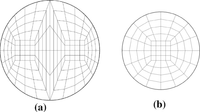
The macro mesh topology of computational domain used in the study. a Mesh topology of the mother branch at section . b Mesh topology of the right daughter branch at section
This resolution results in a mesh of 38,400 elements with a total of 13,171,200 node points. This setup was typically solved using 512 CPUs, with run times of around two weeks to conduct enough cycles of the flow to ensure converged statistics.
Simulation parameters
Since the geometry used is fixed, and the reciprocating flow employed is purely harmonic, the flow can be shown to be a function of only two non-dimensional groups. The first of these essentially quantifies the amplitude of the reciprocating flow, which we define as a maximum Reynolds number as
| 5 |
where is the kinematic viscosity. The second parameter quantifies the frequency, which can be presented in terms of the square of the Womersley number
| 6 |
where f is the frequency of oscillation. This can, in turn be presented in terms of a traditional Stokes parameter
| 7 |
where is the Stokes layer thickness or viscous length, so that
| 8 |
To set these parameters to be clinically relevant we start from the conditions of a typical full-term neonate, which are: volume per inflation per unit body weight of the infant 1–3 ml/kg and the frequency of therapy in the range of 8–12 Hz. The typical diameter of the endotracheal tube employed is 3 mm. Assuming typical numbers of a body mass of 3 kg and a ventilator frequency of 12 Hz results in and at the mother branch of the first generation, referred to here as .
As mentioned in Sect. 1, the structure of the human airway is effectively self-similar, with each generation maintaining similar proportions as shown in Fig. 2 and defined in Grotberg [18]. Therefore, if it is assumed that the flow splits symmetrically in each daughter branch, once the amplitude and frequency (quantified by and ) are known at the first generation, and can be calculated at each subsequent generation. Figure 4 shows the variation of pairs at each generation for the typical neonate conditions outlined above. The same data for the first four generations, and the ninth generation, are also tabulated in Table 1.
Fig. 4.
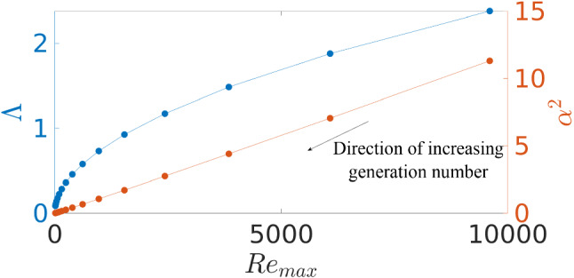
Variation of traditional Stokes parameter , and Womersley number squared , as a function of maximum Reynolds number for generations 1–15 of the neonatal airway, using the proportions proposed by Grotberg [18]
Table 1.
Summary of simulation attributes
| Case | Simulating junction | Re | ||||
|---|---|---|---|---|---|---|
| DNS1 | 50 | 849 | 9600 | 11.31 | 2.38 | |
| DNS2 | 25 | 849 | 9600 | 11.31 | 2.38 | |
| DNS3 | 25 | 861 | 6076 | 7.06 | 1.88 | |
| DNS4 | 25 | 873 | 3846 | 4.41 | 1.48 | |
| DNS5 | 25 | 885 | 2434 | 2.75 | 1.17 | |
| DNS6 | 25 | 950 | 247 | 0.26 | 0.36 |
The maximum local Reynolds number decreases from the predecessor generation to the successive generation by a factor of while the Womersley number decreases from the predecessor generation to the successive generation by a factor of . This reduction of and with increasing generation number i is caused by the reduction of local diameter and local maximum velocity.
We therefore characterize the airflow at a particular airway generation subjected to HFV as a two-parameter problem in the space. In this two-parameter space, we have taken the pairs identified in Fig. 4 to match the conditions at each airway generation and run simulations matching the conditions of the first 10 generations. While this does not produce a complete characterization of the flow (we have obviously removed the coupling between generations and the secondary flows that will be generated by this coupling) it does allow us to provide a first estimate of how the mean streaming and turbulent transport vary quantitatively in different regions of the airway.
There are various dimensionless groups used in the previously reported studies in this context. Table 2 shows relationships among frequently reported dimensionless groups. In the Keulegan–Carpenter number, V is the amplitude of the oscillating flow velocity and T is the period of oscillation. The dimensionless group (a) represents the ratio between the entrance boundary layer thickness and the thickness of the Stokes layer [43] and (b) represents the time-varying ratio between temporal and convective acceleration [27].
Table 2.
Relationships among various dimensionless groups used to describe unsteady reciprocating flow
| Algebraic relationship | Dimensionless group | Dimensionless group as a function of and |
|---|---|---|
| Womersley number squared | ||
| Maximum Reynolds number | ||
| Dean number | ||
| Keulegan–Carpenter number | ||
| Strouhal number | ||
| a | ||
| b | ||
Results and discussion
In this section we present the results of the simulations of the parameter pairs shown in Fig. 4 and Table 1. Throughout, we use the term inhalation to refer to the flow moving from the mother branch to daughter branches, and exhalation to refer to the flow moving in the opposite direction, from daughter branches to the mother branch. Note that these terms here simply indicate flow direction—they do not imply any active or passive changes in pressure as may be the case in a physiological setting. We first present results quantifying the nonlinear mean streaming induced by the reciprocating flow, before investigating the appearance and character of turbulence.
Streaming velocity
In this section, we focus on the quantification of mean streaming. The streaming velocity field is simply the cycle-average of the velocity, . We calculate this mean directly from the simulation by averaging over an integer number of cycles. We excluded the first cycle of the simulation to avoid any initial transient. We also note that any transient did not appear to extend beyond this first cycle, with the statistics of the flow apparently settled from the second cycle onward. This raises an important point—even though the frequency is “high” in a physiological sense, the time scale of the oscillation is still slow compared to the advective time scale . This means that any transient that appears has many advective time units to wash out of the domain even in a single cycle of oscillation.
Figure 5 shows a trace of the axial velocity measured at a point from the bifurcation origin on the center of the mother branch over three cycles of oscillation starting from rest for first generation case, . It is clear that, aside from the details of the turbulent fluctuation (which is discussed in more detail in Sect. 3.5) that the flow is not varying between the second and third cycle.
Fig. 5.
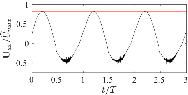
The time history of the velocity measured at a point measured along the abscissa S of the mother branch, for the first three cycles of the case. Horizontal red and blue lines mark minimum and maximum values, showing these values repeat between the second and third cycles. The trace shows that the flow repeats from the second to the third cycle, with no impact from any initial transient present
The streaming velocity field for cases , , and are shown in Fig. 6. This figure presents contours of the mean velocity component aligned with the local axial direction , with positive designating inhalation, with flow moving from the mother to the daughter branches. In each of the four cases, the first panel displays 6 sections perpendicular to the streamwise direction accompanied by a plane passing through centerlines of the mother and daughter branches. The second panel shows the same data without the latter center plane to clearly show the structure on the perpendicular planes. Note that the integral of over an arbitrary cross section is zero as the field is computed from the cycle-average of the zero-net-mass-flux reciprocating flow.
Fig. 6.

Visualization of dimensionless streaming velocity fields for a , (, , ); b , (, , ); c , (, , ); and d , (, , ). The first panel of each case shows the longitudinal symmetry plane along with several transverse planes. The second panel shows the same field without the longitudinal symmetry plane
Figure 6a–c shows qualitatively similar fields among the , and cases. A general characteristic of these three cases is that along the core of the mother branch there is an inhalation streaming flow surrounded by an exhalation streaming, whereas along the core of the daughter branch there is an exhalation streaming surrounded by an inhalation streaming. However, there are clear lobes of higher-magnitude velocity, especially on the planes closest to the bifurcation—four lobes in the mother branch and two lobes in each of the daughter branches, suggestive of the formation of longitudinal vortices.
Figure 7a–c shows qualitatively similar fields among the , and cases. A general characteristic of these three cases is that along the core of the mother branch there are 4 counter-rotating vortices and along the core of the daughter branch there are 2 counter-rotating vortices. These are suggestive of the formation of longitudinal vortices.
Fig. 7.

Visualization of dimensionless axial vorticity computed based on the streaming velocity fields for a , (, , ); b , (, , ); c , (, , ); and d , (, , )
To further investigate this, Fig. 8 shows the transverse velocity vector field superposed on contours of the streaming velocity on sample planes in the mother and daughter branches. The figure clearly shows that the lobes of high coincide with recirculation regions in the secondary flow.
Fig. 8.

Contours of streaming velocity on cross sections A–A and B–B superposed with secondary flow vectors. Note the vectors are uniform length, not scaled by magnitude, and so indicate the flow direction only. Cross sections A–A and B–B are at and measured along respective abscissas from the bifurcation origin
These vortical structures appear to be similar to Dean vortices, the structures formed due to a centrifugal instability in a curved pipe. In a circular pipe of constant curvature, this mechanism causes two vortices which are symmetric about the plane of the curve as fluid is pushed from the inner to outer side of the curve on the plane, and returns along the upper and lower surfaces of the circular pipe [4]. Further, Jan et al. [29] and Jalal et al. [28] have reported these vortices in a bifurcation geometry as well. Here, the instability is caused by the curvature of the flow passing through the bifurcation.
We first focus on the impact of this instability on the flow in the daughter branch. During inhalation, the instability causes the two-vortex system to grow in each daughter branch. Fluid on the centerplane is pushed towards the outer side of the curve of the daughter branches (the side marked B in Fig. 8), and the peak of the axial velocity is also moved in this direction, leaving a velocity deficit at the center of the branch. During exhalation, the impact of the curvature is not felt in the daughter branch, and the velocity profile is effectively axisymmetric. This means that, on average, the exhalation velocity is higher than the inhalation velocity at the center of the daughter branches and in the vortex cores, and as such the mean axial velocity is in the exhalation direction in this region.
Focusing on the impact in the mother branch just beyond the bifurcation, i.e. the area highlighted on plane 2 in Fig. 6a the two-vortex system is generated via the curvature from each of the daughter branches during exhalation, causing two counter-rotating pairs of vortices to enter the mother branch, with fluid from each daughter branch being pushed towards the center of the mother branch on the center plane, and the peak axial velocity also being moved towards the center of the mother branch. During inhalation there is no impact of the curvature in the mother branch so that the exhalation velocity at the very center of the mother branch is higher than the inhalation, and the mean flow in this region is also an exhalation. This is shown, for example, in the planes 1, 2 and 3 in Fig. 6a. Notably however, the direction of the mean flow in the vortex cores, slightly away from the center of the branch is in the opposite direction. Progression up the mother branch away from the bifurcation shows this region of mean exhalation in the very center of the branch is lost, suggesting a coherent vortex structure only extends a finite distance. This is further investigated when considering the temporal evolution and potential influence of turbulence in Sect. 3.5.
The results presented here suggest that the mean streaming flow that has the capacity to transport gas up and down the airway is strongest when the Dean vortex system is strongest. This suggests a potential mechanism to optimize the gas transport, as flows which generate the strongest vortices for the largest proportion of each half cycle (with vortices in the daughter branches during inhalation and the mother branch during exhalation) have the potential to generate the strongest streaming flow. Using a flow cycle that deviates from a pure sinusoid may be one way to impact the strength, and the time of existence, of the vortex system, and hence the strength of the recirculation. The optimization of the pressure waveform to maximize this recirculation is left as a topic of future research.
This general flow structure persists for the upper generations, with the strength of the streaming flow reducing with increasing generation. Figure 6d shows the field for a lower generation case, . This streaming velocity field is much weaker than the former cases and hence, the color map is re-scaled to highlight subtle variations. There is a weak inhalation streaming surrounded by a weak exhalation streaming close to the bifurcation, however, in other regions of the domain, a much weaker exhalation streaming exists in the core.
The basic flow structure reported here—a counter-rotating vortex pair in each daughter branch during inhalation, and two counter-rotating pairs in the mother branch during exhalation—is in agreement with the experimental findings of Jan et al. [29] which also studied a single bifurcation. Interestingly, the four-vortex structure in the mother branch was also observed in the magnetic resonance velocimetry experiment by Jalal et al. [28] on a double bifurcation model. This last comparison suggests that the presence of lower generations does not have a strong impact on the flow structure in the upper generations.
Recirculation
The key measurement that follows from characterizing the mean flow is the amount of recirculating flux. From a gas transport perspective, this is crucial—the more flow that is being recirculated, the higher the rate of transport of gases up and down the airway. Here we quantify the amount of flow recirculated using the positive flux of the cycle-averaged axial velocity field . Essentially, this is computed by integrating over a plane, but only considering the portions where the flow is moving in the positive streamwise direction. Since the overall mean mass flux must be zero, the integral of over the portions where the flow is moving in the negative direction will be equal and opposite to this. The definition of this quantity can be written as
| 9 |
where H is the Heaviside function. This mean recirculating flux is then normalized by the maximum flow rate in the mother branch, . We performed the integration defined in Eq. (9) over a series of planes transverse to the mother and daughter branches, to quantify as a function of the distance from the bifurcation.
Figure 9 shows the variation of normalized recirculation flux as a function of distance measured from the origin of the bifurcation in the cases modeling the first five generations, as well as the example case for the ninth generation . The distance is presented in terms of distance from the origin of the bifurcation as defined in Fig. 2 and normalized by the diameter of the mother branch , measured along the relevant branch centerline. Negative distances indicate a location in the mother branch, positive distances indicate a location in the daughter branch. The basic character of dependence of the flux on the distance is the same in all of the upper generations. In the bifurcation region of mother and daughter branches, there is a maximum around and , respectively, with the amount of flux decaying with increasing distance from the bifurcation. The value of this maximum peak decreases with increasing generation (or decreasing and ), and its location moves closer to the origin.
Fig. 9.
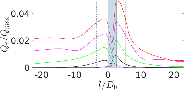
Variation of recirculation flux along the entire flow domain for the cases among , , , , and represented by red, magenta, green, black, gray and blue solid lines, respectively. The dotted lines show locations where neighbor generations would be in a multi-generation bifurcation, and the shading represents the bifurcation region, i.e. the region where the centerlines are curved
A second critical point related to the recirculation is the distance from the bifurcation where the recirculating flux remains significant. In particular, for mean streaming to be a candidate mechanism of gas transport in the airway, the streaming needs to at least reach the location of the next expected generation—in this way the streaming flow from one generation can pass gas up/down to the previous/next generation, and a recirculation chain can be formed to exchange gas in and out of the airway. Figure 9 has the location where neighbor generations up and down the airway would be expected marked with vertical dashed lines (recalling the self-similar geometry of each generation outlined in Sect. 1). Notably, the value of in both the mother and daughter branches at the location of the adjoining generation is approximately the same in a given generation case, and decreases with increasing generation. In the first generation case , the recirculating flux is around , falling to around for the third generation case . By the ninth generation , the recirculating flux is practically zero.
Figure 10 shows the effective strength of recirculating flux for the first nine generations, at the point in the mother branch where the next generation would be expected. The blue curve corresponds to the strength of recirculating flux as measured through a single 1:2 bifurcation.
Fig. 10.
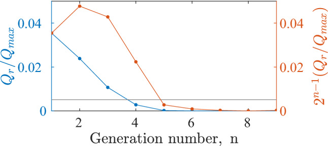
Strength of the recirculating flux passed on to the successive generation as a function of the generation number. The horizontal gray line corresponds to the flow rate required to meet the oxygen demand of a neonate in the clinical conditions based on the data reported by Hill and Robinson [24]
The orange curve is obtained by multiplying this dataset by a factor of (where n is the generation number greater than 0) which represents the number of 1:2 bifurcation units in each generation to compute the total recirculating flux at each “generation level” in the airway. As an important feature of the mean streaming in this context, we report that the strength of recirculating flux is highest in the generations 2 and 3, and gradually decreases in successive generations and becomes negligible beyond the generation 5. The relevance of this streaming recirculation can be assessed by comparing it to the oxygen requirement of a patient. Assuming a oxygen demand of for a neonate in the clinical conditions as reported by Hill and Robinson [24], the amount of gas recirculation required to provide this can be calculated. This amount is marked by the horizontal gray line in Fig. 10. This comparison shows that the amount of oxygen passed on to the successive generation through the steady streaming phenomenon is adequate to meet with the demand up to the generation 4, and only slightly below in generation 5.
The variation in the strength of the streaming can be related to the generation of Dean vortices due to the curvature of the flow through the bifurcation. Figure 11 shows the same recirculating flux data as the blue curve in Fig. 9, i.e. the recirculating flux in a single bifurcation, but plotted as a function of rather than generation number. Further, the two subfigures plot the same data, first on a linear scale and then on a logarithmic scale.
Fig. 11.

Dimensionless recirculating flux as a function of for the first 9 generations. a The red curve shows a power law fit for the first 4 generations with the power . b The red straight line shows a linear fit for the semilog data of the generations 5–9 where generation 8 is ignored as an outlier of the linear fit
We note that plotting as a function of ignores the impact of —we are suggesting that since is always low (with in the first generation case and reducing for subsequent generations) its impact is weak. This is perhaps not surprising if is considered as a ratio of length scales as shown explicitly in Eq. (8) where is shown to be proportional to the ratio of the pipe diameter and the viscous length . In the classic infinite-length straight pipe, the viscous length is interpreted as the Stokes layer thickness. In that case it is easier to see why the impact of is weak when is small. A small implies a large Stokes layer thickness; in a pipe, this layer thickness cannot physically exceed the pipe radius; so reductions in that have a corresponding increase in cease to have an impact.
The interpretation for flows with greater geometric complexity is perhaps not as clear, but the same general argument can be presented. The recent study of the reciprocating flow in a straight pipe, but with a free end in a large reservoir [20], reached a similar conclusion—the flow response could be split into low- and high- regimes, driven by the self-interaction of toroidal vortices formed at the free end of the pipe. In that case, the viscous length is proportional to the Stokes layers in the pipe but also the vortex core size.
In the flow studied here, there are neither well-defined Stokes layers or toroidal vortices in the vicinity of the bifurcation. The primary flow features are the Dean vortices, and is perhaps related to their core diameter. We suggest therefore that a similar argument to the above can be presented, that while is low, this viscous length is saturated and therefore variations in have little effect, leaving as the parameter which effectively determines the flow behaviour.
Clear regimes can be identified in Fig. 11 as a function of . The data on the linear scale show significant streaming for , with the normalised recirculating flux varying like for values above this threshold. The same data on a logarithmic scale show that for , the recirculating flux varies exponentially (linearly on the logarithmic scale) with .
We suggest this change in regime is related to the generation of distinct, separated Dean vortices. For the high- regime, the generation of these vortices leads to a nonlinear relationship between and the strength of the streaming flow. For the low- regime, these distinct vortices are not formed, and the strength of the streaming flow decays exponentially with decreasing .
This is supported by the flow visualisation in terms of vorticity presented in Fig. 7. For the higher cases, distinct vortical structures are present in the streaming field, whereas these are not present in the lower cases.
Figure 9 shows that the streaming flow can potentially deliver gas over the distance by which subsequent generations are separated. Here, we investigate this recirculating distance further.
Figure 12 shows a shear stress magnitude distribution, on the walls of the domain calculated from for the first generation case . Note that is not the mean stress, however this quantity should be zero an any segment of the geometry where there is no mean streaming. The magnitude of is high in the bifurcation region where the streaming flow is strongest, and it gradually decreases to zero along the daughter branches. In contrast, in the mother branch remains high on the top and bottom of the domain while it is low on the sides. It does not settle back to zero along the mother branch, with a significant shear stress extending all the way to the free end, indicating that a streaming flow is present even at distances of 50D from the bifurcation.
Fig. 12.

Distribution of wall shear stress based on the streaming velocity field for (, , )
To further quantify this, Figs. 13 and 14 show the variation of measured along the centerline of the mother and daughter branches for flows for different generation cases. Along the centerline of the mother branch, the axial velocity is almost identical with the magnitude of the overall mean velocity , implying that the mean transverse velocity is almost negligible (at least on the centerline). Both figures indicate that the field progressively weakens for each subsequent generation case, and is negligible by the case. However, in all the generation cases passes through a local minimum at a distance around , but then rapidly increases to meet with a local maximum at around . In the first generation case this is followed by a short plateau, subsequently followed by an exponential decay—in the other generations, this plateau is not observed and simply begins to decay after passing the maximum. Notable is the fact that this decay is very slow—at a location around 25D from the bifurcation, on the centerline is still around of its peak value for the first three generations. This is despite the boundary condition that is applied at the free end (the Womersley solution for laminar reciprocating flow in a straight tube) having a zero mean flow.
Fig. 13.
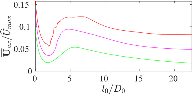
Quantification of recirculation length on the mother branch: variation of measured along the abscissa S among , , and represented by red, magenta, green and blue solid lines, respectively. denotes the distance measured along the centerline of the mother branch from the bifurcation origin (see Fig. 2). Note that the magnitude of the streaming velocity measured along the abscissa S is coincident with suggesting that is negligible in this region
Fig. 14.
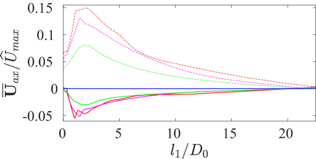
Quantification of recirculation length on the left daughter branch. Variation of measured along the abscissa among , , and represented by red, magenta, green and blue solid lines, respectively. denotes the distance measured along the centerline of the left daughter branch from the bifurcation origin (see Fig. 2). Further, the magnitude of the streaming velocity measured along the abscissa is shown by respective dashed lines. This data is statistically examined among both daughter branches and equivalence is verified
In the daughter branches, there is a complex relationship between the mean flow and distance in the initially curved portion of the branch leaving the bifurcation. Beyond this curved region where , decays effectively exponentially to zero at .
Such long relaxation distances imply that there is a recirculating mean flow extending all the way to the domain boundaries, and this raises the potential of the influence of the boundary conditions on the results. We have investigated this impact and confirmed that the domain size has practically no impact on the location and magnitudes of the maximum streaming in the mother branch, and only a weak impact on the magnitude of the maximum streaming in the daughter branches. Further details of this domain size investigation are presented in “Appendix’.
Instantaneous events impacting the mean structure
In Sect. 3.1, it was argued that the features in the mean flow were driven by the presence of centrifugal-instability generated vortices, reminiscent of Dean vortices, leaving the bifurcation. Here, we show details of the temporal evolution of the flow confirming this argument and showing these Dean vortices explicitly.
A dominant feature that accompanies the development of the Dean vortices is the onset of conditional turbulence in the upper generations which is a function of the generation number. The preceding sections have shown that this has little impact on the trend of the streaming flow with different generation number, indicating that it is the large-scale flow structures that drive the streaming. We also show that is the Dean vortices themselves that are the necessary condition for the generation of this turbulence, and the mechanism of the onset of turbulence in the reciprocating flow in the bifurcation is different to that in a constant-flow, or reciprocating-flow, straight pipe flow, which may have implications for the construction of low-order models that attempt to incorporate turbulence effects (see, for example Herrmann et al. [23]).
Figure 15 shows 9 panels of vortical structures constructed based on the criterion [30], which defines vortex cores as any region where . Each panel illustrates iso-surfaces of these vortical structures based on the threshold value of . Three panels in the first row, a1, a2 and a3 correspond to iso-surfaces generated based on the mean streaming velocity field of , and cases, respectively. Similarly, three panels in the second row, b1, b2 and b3 correspond to iso-surfaces generated based on the peak inhalation flow field of , and cases, respectively. Further, three panels in the third row, c1, c2 and c3 correspond to iso-surfaces generated based on the peak exhalation flow field of , and cases, respectively.
Fig. 15.

Isosurfaces of vortical structures based on the threshold value of . a1–a3 correspond to iso-surfaces generated based on the streaming velocity field of , and cases, respectively. Similarly, b1–b3 correspond to iso-surfaces generated based on the peak inhalation flow field of , and cases, respectively. Further, c1–c3 correspond to iso-surfaces generated based on the peak exhalation flow field of , and cases, respectively
The mean flows shown in the first row appear at first glance inconsistent. The streamwise vortical structures apparent in the mean velocity and vorticity contours in Figs. 6 and 7, and the secondary flow vectors in Fig. 8 do not appear in the field for the first generation case, and appear to strengthen with increasing generation, despite the streaming flow weakening (as demonstrated by the recirculating flux presented in Fig. 9). This suggests there is a process—conditional turbulence—that destroys the coherence of the mean vortex structures such that they are not reliably detected using the criterion.
Evidence of this process—the appearance of conditional turbulence growing on these streamwise vortex structures—is clear in the subsequent images in Fig. 15. The second row of images shows the isosurfaces at peak inhalation. During the inhalation half-cycle, two vortical structures progressively enlarge along the flow direction, which are the two counter-rotating vortices generated by centrifugal instability in the curved section of the bifurcation entering each daughter branch. These structures are clear in the images (b2) and (b3) for the second and third generation cases, respectively. However, the first generation case shows a much more complex structure, with the daughter branches being filled with small scale turbulent eddies.
A similar process occurs during exhalation. Again, two counter-rotating vortices are formed from the centrifugal instability induced by the curvature of the bifurcation where the flow is leaving each daughter branch. This results in two counter-rotating pairs, or four streamwise vortices, entering the mother branch. This four-vortex system is clearly apparent in the image (c3) for the third generation case. However, image (c2) for the second generation case shows this structure already breaking down to much finer scale, apparently turbulent vortex structures, and the first generation again shows the flow breaking down into small scale turbulent eddies that fill the entire mother branch.
Taken together, the images in Fig. 15 suggest that in the first generation case, turbulence develops in both the mother and daughter branches, but only in the flow leaving the bifurcation, i.e. turbulence occurs in the daughter branches during inhalation and in the mother branch during exhalation. The appearance of turbulence coincides with the development of the streamwise vortex structures leaving the bifurcation, and we propose that this turbulence occurs via an instability of this vortex system.
This idea is consistent with the data. The second generation case also shows the development of turbulence, but only in the mother branch during exhalation. Here the turbulence develops on the four-vortex system, but not on the two-vortex systems in the daughter branches. We investigate the onset of this turbulent structure and its potential mechanism of generation in the following sections.
Instantaneous velocity
Here, we investigate the complex temporal variation of the flow, especially in the first and second generation cases that appear conditionally turbulent.
We first focus on the evolution of the instantaneous velocity field over a complete cycle of the pulsatile flow. Figures 16 and 17 show contours of velocity magnitude along the bifurcation (mid plane) among and for 12 consecutive phases of the cycle. For conciseness and clarity of the instantaneous flow visualizations, only one half of the fluid domain is shown in each panel. These velocity fields were indeed verified to be statistically symmetric around the bifurcation centerline ( axis). The first and the last panels correspond to and , respectively, with an interval of phase angle between each consecutive panel. The upper 6 panels of each figure corresponds to the inhalation half cycle while the lower 6 panels correspond to exhalation.
Fig. 16.

Evolution of the instantaneous velocity magnitude, for (, , ). The dotted lines highlight areas where turbulent bursts have developed in the flow
Fig. 17.

Evolution of the instantaneous velocity magnitude, for (, , ). The dotted lines show turbulent bursts developed in the flow
Figure 16 shows that in the first generation case , during the first quarter of the cycle (acceleration phase during which the inhalation flow rate increases with time), a high momentum region progressively develops in the mother branch and propagates along the walls at the outside of the curve of the daughter branches. Turbulence appears downstream of the bifurcation, approximately from measured along the daughter branches when . This turbulence appears to be sustained for as depicted from panels 3–5 of Fig. 16. In the second quarter of the cycle (deceleration phase during which the inhalation flow rate decreases with time), the turbulence decays and the flow relaminarizes when the flow velocity decreases below a critical value as shown in panels 5–6.
Figure 17 shows that during inhalation, there is no turbulence observed in the case. This implies that turbulence is also not observed in the daughter branches for further generations. The deceleration phase sees the high momentum region deplete gradually and disappear at the inversion between inhalation and exhalation as shown in panels 4–6.
The exhalation phase is more similar between the two cases. In the third quarter of the cycle (acceleration phase during which the exhalation flow rate increases with time), the flow streams from daughter branches to the mother branch merge, and a jet-like high momentum region is created and propagates along the core of the mother branch. As depicted by the lower panels of Figs. 16 and 17, this high momentum region undergoes an instability leading to a turbulent flow appearing beyond the bifurcation, approximately from measured along the mother branch, and in the center of the pipe. Both generation cases demonstrate a qualitatively similar behaviour yet the turbulent intensity is highest in the case. In the final quarter during which the exhalation flow rate decreases with time, the turbulence decays and the flow relaminarizes while the high momentum region depletes gradually to facilitate the flow inversion for the next cycle.
Next we focus on the evolution of basic streamwise vortex structure influenced by the presence of turbulence for case. Figures 18 and 19 show contours of axial vorticity along cross sections A–A and B–B, respectively (note that the length of the vectors are not scaled by the magnitude). The first and the last panel of each figure correspond to and , respectively, with an interval of phase angle between each consecutive panel. The first 6 panels of each figure corresponds to the inhalation half cycle while the next 6 panels correspond to exhalation.
Fig. 18.

Evolution of the axial vorticity along cross section A-A for (, , ). The cross section A-A is at measured from the bifurcation origin on the mother branch
Fig. 19.

Evolution of the axial vorticity along cross section B–B for (, , ). The cross section B–B is at measured from the bifurcation origin on the right daughter branch
As revealed by Fig. 18, pertaining to the mother branch, there is no apparent vortical structure developed during the inhalation half-cycle. However, there are four counter-rotating vortices (two counter rotating vortex pairs that are symmetric around the plane) at the start of the exhalation half-cycle and persisted for under the influence of turbulence and eventually disappeared with the inversion of the flow.
According to Fig. 19 pertaining to daughter branches, there are two counter rotating vortices (a counter-rotating vortex pair) that are symmetric around the plane appeared at the start of the inhalation cycle that persist for , even under the influence of turbulence. They eventually weaken and disappear with the inversion of the flow. There is no apparent vortical structure developed during the exhalation half-cycle.
The basic streamwise vortex structure indicated here explains why the recirculating flux is highest in the uppermost airway generation, but the streamwise vortices are not apparent in the mean flow when viewed with the criterion. This indicates that even if the turbulence occurs in the upper airway, it does not have a noticeable impact on the mean streaming, as the mean velocity field has not been influenced by the turbulence. This feature of the flow leads to an important result from a clinical point of view: the impact of mean streaming on HFV can be controlled by manipulating the input pressure waveform to maximize the vortex structure regardless of the appearance of turbulence.
Further details of conditional turbulence
To study the temporal variation of the instantaneous velocity field, the history of the velocity at specific locations in the flow domain are recorded for the first generation case . Figure 20a, b illustrates the history of the axial velocity at and measured along the abscissas S and , respectively. The first point is located in the mother branch, the second point is located in the left daughter branch ( fields have been verified to be statistically equivalent for left and right daughter branches). Three curves are shown in each plot. The first shows the raw history of the axial velocity (in black). The second and third show the axial velocity low-pass (in green) and high-pass (in red) filtered, using a cut-off frequency of (note the frequency of the cycle for this first generation case is ). This decomposition facilitates us to quantify the time duration for which turbulence prevails.
Fig. 20.
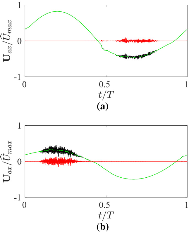
A decomposition of the velocity time history. a Decomposition of temporal velocity data at measured along the abscissa S. b Decomposition of temporal velocity data at measured along the abscissa . Solid line shows the measured temporal data from the instantaneous velocity field; solid line shows the velocity scale associated with the filtered low-frequency components while the solid line shows the velocity scale associated with the filtered high-frequency components. The cut-off frequency for the low- and high-pass filters was
Figure 20 clearly shows the appearance of turbulent bursts in both the mother and daughter branches, centered around an epoch of time where the flow rate is close to maximum—during exhalation in the mother branch (maximum negative flow rate), and inhalation in the daughter branch (maximum positive flow rate). We note here that this is in contrast to the behaviour in the reciprocating flow in a straight tube. In a straight tube, it has been shown the turbulent bursts typically occur at epochs centered around the peak deceleration [1, 25]. Stability analysis of the straight tube flow indicates that these bursts do not occur via a linear instability [6, 48], but rather through the transient amplification of disturbances at the tube walls, effectively in the Stokes layers [2, 33, 50]. The fact that we have observed turbulence at a different point in the cycle and clearly growing nearer the center of the pipe than the walls indicates that the transition mechanism here is not the same as that in the straight tube.
To further investigate the spatio-temporal dependence of the appearance of turbulent bursts, Fig. 21 presents space-time diagrams of the axial velocity measured along the abscissa of both the mother and daughter branches for the first generation case. Note the high-pass filtered data is used to remove the effect of the base reciprocating flow, and the data is spatially filtered (eliminating low wavenumbers) again to remove any mean trend. This figure confirms the findings from Fig. 20 that the turbulent bursts occur at an epoch near the maximum flow rate. They also show the spatial extent of the turbulent patches. In the mother branch, the fine-scale turbulent structure is focused in a patch around 3D from the bifurcation, however there is apparent turbulent structure extending much further with turbulence evident over the entire extent of the plot (25D). In the daughter branch, there is an initial periodic structure attributable to the two streamwise vortices emanating from the curved region of the bifurcation, before a turbulent patch occurs that starts approximately from the origin—just beyond the end of the curved section of the bifurcation. This patch decays by around , with weak turbulent structure again apparent over the entire range of the plot.
Fig. 21.

Space–time diagram of spatially filtered (high wavenumber) and temporally filtered (high frequency) components of for (, , ). a Contours of filtered components of plotted in the space-time coordinates of the mother branch. b Contours of filtered components of plotted in the space-time coordinates of the daughter branch. c The spatially averaged velocity implemented as the inlet boundary condition which is proportional to the flow rate. The vertical dashed line shown in the panel (b) represents the end of the curved section of the bifurcation
Another feature that is clear in the space-time diagrams of Fig. 21 is the fact that the turbulent bursts only occur in the flow leaving the bifurcation. This is despite the fact that is well above the value required for transition to turbulence of the steady flow in a pipe [3, 10] in the first generation case, and the instantaneous Reynolds number is above the transition value of a large part of the oscillation cycle. This indicates that the instantaneous flow profiles deviate from the parabolic Poiseuille profile that would be expected if the instantaneous flow rate was applied to a steady flow. Figure 22 shows a quantitative comparison between equivalent Womersley and Poiseuille profiles. The variation of cross-sectionally averaged velocity (bulk velocity) over a flow cycle is shown in blue. The orange curve displays the root mean squared difference between the Poiseuille profile for the instantaneous value of bulk velocity, and the imposed Womersley profile at the same instant. This comparison provides an indication of how much the Womersley profile deviates from the quasi steady assumption over a complete flow cycle. It shows that near the peak flow rate, the difference is not large, however this is only true for a very short time, and the true profile differs considerably from the Poiseuille profile over the majority of the oscillation cycle. This provides some indication as to why the turbulence is only seen in the flow leaving the bifurcation—the laminar flow profile entering the bifurcation deviates from the steady flow profile enough to suppress the transition mechanisms that occur in the steady flow, and only the instability of the streamwise vortices generated by the bifurcation curvature lead to turbulence.
Fig. 22.
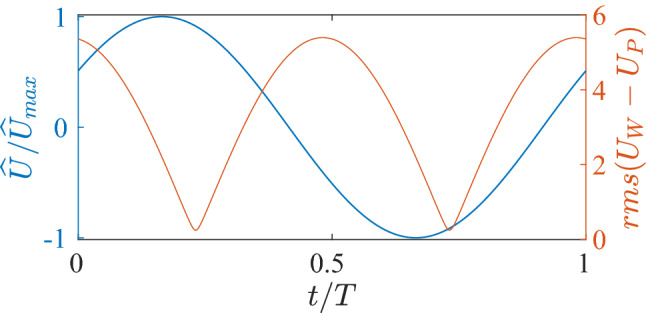
Temporal variation of cross sectionally averaged (bulk) velocity implemented as the inlet boundary condition is shown in blue and rms of deviation of inlet velocity profile from the Poiseuille profile with the same flow rate is shown in orange
Conclusion
Direct numerical simulation has been used to model airflow in the neonatal airway subjected to clinically relevant conditions of HFV. Among several gas transport mechanisms that could play a role in HFV, our focus has been on quantifying the effect of nonlinear mean streaming. Although the oscillatory flow in a single bifurcation model has been extensively studied before, the high-resolution volumetric data obtained in the present study provide important insights to the flow evolution in the context of clinically relevant HFV parameters used in the NICU.
In this context, we report that the nonlinear mean streaming plays a significant role in the gas transport of the upper airway. In fact, the recirculating flux can be up to 5% of the maximum flow rate in the trachea and primary bronchi (generation cases and ). Our calculations reveal that for conditions relevant to the first four generations of the upper airway, the amount of oxygen supplied through this phenomenon likely meets the anticipated oxygen demand of a neonate.
As an important feature of the flow, turbulent bursts observed downstream of the bifurcating junction when the flow speed exceed a critical value and relaminarizes periodically when the flow speed decreases below the critical value. During the inhalation, this conditional turbulence is observed in the daughter branches whereas it is observed in the mother branch during the exhalation. We believe that turbulent bursts are caused by the instability of the vortical structures elongated along the flow direction downstream of the bifurcating junction. A comprehensive stability analysis of this flow field might be of value. Notably, this conditional turbulence is only observed in the first three generations of the upper airway as the flow speed progressively decreases further down the airway.
Acknowledgements
We thank anonymous reviewers for providing comprehensive, insightful comments that led to a much improved final manuscript. CJ acknowledges the joint financial support of Swinburne University of Technology and the Murdoch Children’s Research Institute via the growth SUPRA scheme. This work was performed on the OzSTAR national facility at Swinburne University of Technology. OzSTAR is funded by Swinburne University of Technology and the National Collaborative Research Infrastructure Strategy (NCRIS). DGT is supported by a National Health and Medical Research Council Career Development Fellowship (1123859) and the Victorian Government Operational Infrastructure Support Program. The authors thank Ravindu Jayagoda for preparing CAD models.
Appendix: Impact of domain size on the mean recirculation
To investigate any potential effect of domain size, we have quantified along the centerline of each branch for two different domain sizes. In the second domain, the bifurcation region was identical geometrically to that of the first (as outlined in Fig. 2) while the branch lengths for both the mother and daughter branches were doubled (). The data sets from the two domains showing on the mother and daughter branches for the first generation case are shown in Fig. 23.
Fig. 23.
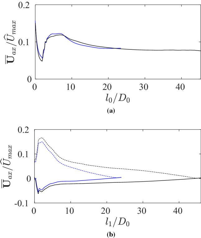
Results of DNS1 and DNS2 as the domain test for two different domain lengths () for the first generation case. Blue lines represent the data from the original simulation, black lines represent the data from a simulation on the longer domain. a Variation of along the centerline of the mother branch for different domain lengths. b Variation of along the centerline of daughter branches for different domain lengths
Focusing first on the mother branch, Fig. 23a shows that there is a very small effect of the domain size on the streaming flow. However the location of local minima and maxima are almost the same with only a small difference in magnitude.
Focusing on the daughter branch in Fig. 23b shows a stronger effect of the domain. Similar to the mother branch data, the location of local minima and maxima are practically unchanged between the two domains. However, the magnitude of the local maximum is impacted, as is the decay of the centerline velocity from this maximum back to zero. The magnitude of the maximum is larger in the longer domain, and in both domains the velocity decays to approximately zero at the end of the domain, meaning the decay is slower in the longer domain. This indicates that there is a weak effect of the modified outflow condition applied to the free end of the daughter branches. However, the effect is weak in the area of interest (near the bifurcation)—for example, at 10D, the original domain gives a value of , whereas the longer domain gives a value of . This difference is acceptable, noting that the next generation would be expected at a distance around 3.5D.
Footnotes
Publisher's Note
Springer Nature remains neutral with regard to jurisdictional claims in published maps and institutional affiliations.
References
- 1.Akhavan R, Kamm R, Shapiro A. An investigation of transition to turbulence in bounded oscillatory Stokes flows part 1. Experiments. J. Fluid Mech. 1991;225:395–422. doi: 10.1017/S0022112091002100. [DOI] [Google Scholar]
- 2.Akhavan R, Kamm R, Shapiro A. An investigation of transition to turbulence in bounded oscillatory Stokes flows part 2. Numerical simulations. J. Fluid Mech. 1991;225:423–444. doi: 10.1017/S0022112091002112. [DOI] [Google Scholar]
- 3.Avila K, Moxey D, de Lozar A, Avila M, Barkley D, Hof B. The onset of turbulence in pipe flow. Science. 2011;333:192–195. doi: 10.1126/science.1203223. [DOI] [PubMed] [Google Scholar]
- 4.Berger S, Talbot L, Yao LS. Flow in curved pipes. Annu. Rev. Fluid Mech. 1983;15:461–412. doi: 10.1146/annurev.fl.15.010183.002333. [DOI] [Google Scholar]
- 5.Bhosale, Y., Parthasarathy, T., Gazzola, M.: Shape curvature effects in viscous streaming. arXiv preprint arXiv:1912.03816 (2019)
- 6.Blennerhassett P, Bassom A. The linear stability of high-frequency oscillatory flow in a channel. J. Fluid Mech. 2006;556:1–25. doi: 10.1017/S0022112006009141. [DOI] [Google Scholar]
- 7.Budwig, R.: Two unsteady heat transfer experiments: (i) in grid-generated isotropic turbulence; (ii) in laminar oscillatory flow in straight and conical tubes. PhD thesis, John Hopkins University (1985)
- 8.Chang H. Mechanisms of gas transport during ventilation by high-frequency oscillation. J. Appl. Physiol. 1984;56(3):553–563. doi: 10.1152/jappl.1984.56.3.553. [DOI] [PubMed] [Google Scholar]
- 9.Choi J, Xia G, Tawhai MH, Hoffman EA, Lin CL. Numerical study of high-frequency oscillatory air flow and convective mixing in a CT-based human airway model. Ann. Biomed. Eng. 2010;38(12):3550–3571. doi: 10.1007/s10439-010-0110-7. [DOI] [PMC free article] [PubMed] [Google Scholar]
- 10.Eckhardt B, Schneider T, Hof B, Westerweel J. Turbulence transition in pipe flow. Annu. Rev. Fluid Mech. 2007;39:447–468. doi: 10.1146/annurev.fluid.39.050905.110308. [DOI] [Google Scholar]
- 11.El Khoury GK, Schlatter P, Noorani A, Fischer PF, Brethouwer G, Johansson AV. Direct numerical simulation of turbulent pipe flow at moderately high Reynolds numbers. Flow Turbul. Combust. 2013;91(3):475–495. doi: 10.1007/s10494-013-9482-8. [DOI] [Google Scholar]
- 12.Emery J. The Anatomy of the Developing Lung. Oxford: Butterworth-Heinemann; 2014. [Google Scholar]
- 13.Fischer, P.F., Lottes, J.W., Kerkemeier, S.G.: Nek5000 web page (2008)
- 14.Fischer PF, Loth F, Lee SE, Lee SW, Smith DS, Bassiouny HS. Simulation of high-Reynolds number vascular flows. Comput. Methods Appl. Mech. Eng. 2007;196(31–32):3049–3060. doi: 10.1016/j.cma.2006.10.015. [DOI] [Google Scholar]
- 15.Gatlin B, Cuicchi C, Hammersley J, Olson D, Reddy R, Burnside G. Computational simulation of steady and oscillating flow in branching tubes. Proc. ASME FED Symp. Biomed. Fluids Eng. 1995;212:1–8. [Google Scholar]
- 16.Gaver DP, Grotberg JB. An experimental investigation of oscillating flow in a tapered channel. J. Fluid Mech. 1986;172:47–61. doi: 10.1017/S0022112086001647. [DOI] [Google Scholar]
- 17.Gerstmann DR, Minton SD, Stoddard RA, Meredith KS, Monaco F, Bertrand JM, Battisti O, Langhendries J, Francois A, Clark RH. The provo multicenter early high-frequency oscillatory ventilation trial: improved pulmonary and clinical outcome in respiratory distress syndrome. Pediatrics. 1996;98(6):1044–1057. doi: 10.1542/peds.98.6.1044. [DOI] [PubMed] [Google Scholar]
- 18.Grotberg JB. Volume-cycled oscillatory flow in a tapered channel. J. Fluid Mech. 1984;141:249–264. doi: 10.1017/S0022112084000823. [DOI] [Google Scholar]
- 19.Grotberg J. Pulmonary flow and transport phenomena. Annu. Rev. Fluid Mech. 1994;26(1):529–571. doi: 10.1146/annurev.fl.26.010194.002525. [DOI] [Google Scholar]
- 20.Hasan M, Manasseh R, Leontini J. Energy loss and developing length during reciprocating pipe flow in a pipe with a free end. Phys. Fluids. 2020;32(8):083602. doi: 10.1063/5.0011701. [DOI] [Google Scholar]
- 21.Haselton F, Scherer P. Flow visualization of steady streaming in oscillatory flow through a bifurcating tube. J. Fluid Mech. 1982;123:315–333. doi: 10.1017/S0022112082003085. [DOI] [Google Scholar]
- 22.Heraty, K.B., Laffey, J.G.: Quinlan NJ (2008) Fluid dynamics of gas exchange in high-frequency oscillatory ventilation: in vitro investigations in idealized and anatomically realistic airway bifurcation models. Ann. Biomed.l Eng. 36(11) (1856) [DOI] [PubMed]
- 23.Herrmann J, Tawhai MH, Kaczka DW. Parenchymal strain heterogeneity during oscillatory ventilation: why two frequencies are better than one. J. Appl. Physiol. 2018;124:653–663. doi: 10.1152/japplphysiol.00615.2017. [DOI] [PMC free article] [PubMed] [Google Scholar]
- 24.Hill JR, Robinson D. Oxygen consumption in normally grown, small-for-dates and large-for-dates new-born infants. J. Physiol. 1968;199(3):685–703. doi: 10.1113/jphysiol.1968.sp008673. [DOI] [PMC free article] [PubMed] [Google Scholar]
- 25.Hino M, Sawamoto M, Takasu S. Experiments on transition to turbulence in an oscillatory pipe flow. J. Fluid Mech. 1976;75(2):193–207. doi: 10.1017/S0022112076000177. [DOI] [Google Scholar]
- 26.Horsfield K, Dart G, Olson DE, Filley GF, Cumming G. Models of the human bronchial tree. J. Appl. Physiol. 1971;31(2):207–217. doi: 10.1152/jappl.1971.31.2.207. [DOI] [PubMed] [Google Scholar]
- 27.Isabey D, Chang H. Steady and unsteady pressure-flow relationships in central airways. J. Appl. Physiol. 1981;51(5):1338–1348. doi: 10.1152/jappl.1981.51.5.1338. [DOI] [PubMed] [Google Scholar]
- 28.Jalal S, Van de Moortele T, Nemes A, Amili O, Coletti F. Three-dimensional steady and oscillatory flow in a double bifurcation airway model. Phys. Rev. Fluids. 2018;3(10):103101. doi: 10.1103/PhysRevFluids.3.103101. [DOI] [Google Scholar]
- 29.Jan D, Shapiro A, Kamm R. Some features of oscillatory flow in a model bifurcation. J. Appl. Physiol. 1989;67(1):147–159. doi: 10.1152/jappl.1989.67.1.147. [DOI] [PubMed] [Google Scholar]
- 30.Jeong J, Hussain F. On the identification of a vortex. J. Fluid Mech. 1995;285:69–94. doi: 10.1017/S0022112095000462. [DOI] [Google Scholar]
- 31.Lee SE, Lee SW, Fischer PF, Bassiouny HS, Loth F. Direct numerical simulation of transitional flow in a stenosed carotid bifurcation. J. Biomech. 2008;41(11):2551–2561. doi: 10.1016/j.jbiomech.2008.03.038. [DOI] [PMC free article] [PubMed] [Google Scholar]
- 32.Lunkenheimer, P., Rafflenebell, W., Keller, H., Frank, I., Dichut, H., Fuhrmann, C.: Application of transtracheal pressure oscillations as a modification of “diffusion respiration”. BJA Br. J. Anaesth. 44(6), 627627 (1972) [DOI] [PubMed]
- 33.Luo J, Wu X. On the linear stability of a finite stokes layer: instantaneous versus Floquet modes. Phys. Fluids. 2010;22:054106. doi: 10.1063/1.3422004. [DOI] [Google Scholar]
- 34.Mammel M, Courtney S. High-frequency ventilation. In: Goldsmith J, Karotin E, Keszler M, Suresh G, editors. Assisted Ventilation of the Neonate: An Evidence-Based Approach to Newborn Respiratory Care. 6. Amsterdam: Elsevier; 2016. [Google Scholar]
- 35.Mandelbrot BB. The Fractal Geometry of Nature. 3. New York: Henry Holt and Company; 1983. [Google Scholar]
- 36.Marini JJ. Evolving concepts in the ventilatory management of acute respiratory distress syndrome. Clin. Chest Med. 1996;17(3):555–575. doi: 10.1016/S0272-5231(05)70331-2. [DOI] [PubMed] [Google Scholar]
- 37.Menon A, Weber M, Chang H. Model study of flow dynamics in human central airways. Part iii: Oscillatory velocity profiles. Respir. Physiol. 1984;55(2):255–275. doi: 10.1016/0034-5687(84)90026-4. [DOI] [PubMed] [Google Scholar]
- 38.Parthasarathy T, Chan FK, Gazzola M. Streaming-enhanced flow-mediated transport. J. Fluid Mech. 2019;878:647–662. doi: 10.1017/jfm.2019.643. [DOI] [Google Scholar]
- 39.Peattie R, Schwarz W. Experimental investigation of oscillatory flow through a symmetrically bifurcating tube. J. Biomech. Eng. 1998;120(5):584–593. doi: 10.1115/1.2834748. [DOI] [PubMed] [Google Scholar]
- 40.Pedley T, Kamm R. The effect of secondary motion on axial transport in oscillatory tube flow. J. Fluid Mech. 1988;193:347–367. doi: 10.1017/S0022112088002174. [DOI] [Google Scholar]
- 41.Rimensberger PC. ICU cornerstone: high frequency ventilation is here to stay. Crit. Care. 2003;7(5):342. doi: 10.1186/cc2327. [DOI] [PMC free article] [PubMed] [Google Scholar]
- 42.Schlichting H, Gersten K. Boundary Layer Theory. 9. Berlin: Springer; 2017. [Google Scholar]
- 43.Schroter R, Sudlow M. Flow patterns in models of the human bronchial airways. Respir. Physiol. 1969;7(3):341–355. doi: 10.1016/0034-5687(69)90018-8. [DOI] [PubMed] [Google Scholar]
- 44.Sharp MK, Kamm R, Shapiro A, Kimmel E, Karniadakis G. Dispersion in a curved tube during oscillatory flow. J. Fluid Mech. 1991;223:537–563. doi: 10.1017/S0022112091001544. [DOI] [Google Scholar]
- 45.Sklar M, Fan E, Goligher E. High-frequency oscillatory ventilation in adults with ARDS: past, present and future. Chest. 2017;152(6):1306–1317. doi: 10.1016/j.chest.2017.06.025. [DOI] [PubMed] [Google Scholar]
- 46.Standiford T, Morganroth M. High-frequency ventilation. Chest. 1989;96(5):1380–1389. doi: 10.1378/chest.96.6.1380. [DOI] [PubMed] [Google Scholar]
- 47.Tanaka G, Ogata T, Oka K, Tanishita K. Spatial and temporal variation of secondary flow during oscillatory flow in model human central airways. J. Biomech. Eng. 1999;121(6):565–573. doi: 10.1115/1.2800855. [DOI] [PubMed] [Google Scholar]
- 48.Thomas C, Bassom A, Blennerhassett P. The linear stability of oscillating pipe flow. Phys. Fluids. 2012;24:014106. doi: 10.1063/1.3675899. [DOI] [Google Scholar]
- 49.Tufo, H.M., Fischer, P.F.: Terascale spectral element algorithms and implementations. In: SC’99: Proceedings of the 1999 ACM/IEEE Conference on Supercomputing. IEEE, p. 6868 (1999)
- 50.Vittori G, Verzicco R. Direct simulation of transition in an oscillatory boundary layer. J. Fluid Mech. 1998;371:207–232. doi: 10.1017/S002211209800216X. [DOI] [Google Scholar]
- 51.Womersley JR. Method for the calculation of velocity, rate of flow and viscous drag in arteries when the pressure gradient is known. J. Physiol. 1955;127(3):553–563. doi: 10.1113/jphysiol.1955.sp005276. [DOI] [PMC free article] [PubMed] [Google Scholar]