The nature of metacognitive inefficiency in perceptual decision making

Abstract

Humans have the metacognitive ability to judge the accuracy of their own decisions via confidence ratings. A substantial body of research has demonstrated that human metacognition is fallible but it remains unclear how metacognitive inefficiency should be incorporated into a mechanistic model of confidence generation. Here we show that, contrary to what is typically assumed, metacognitive inefficiency depends on the level of confidence. We found that, across five different datasets and four different measures of metacognition, metacognitive ability decreased with higher confidence ratings. To understand the nature of this effect, we collected a large dataset of 20 subjects completing 2,800 trials each and providing confidence ratings on a continuous scale. The results demonstrated a robustly nonlinear zROC curve with downward curvature, despite a decades-old assumption of linearity. This pattern of results was reproduced by a new mechanistic model of confidence generation, which assumes the existence of lognormally-distributed metacognitive noise. The model outperformed competing models either lacking metacognitive noise altogether or featuring Gaussian metacognitive noise. Further, the model could generate a measure of metacognitive ability which was independent of confidence levels. These findings establish an empirically-validated model of confidence generation, have significant implications about measures of metacognitive ability, and begin to reveal the underlying nature of metacognitive inefficiency.

Humans have the metacognitive ability to use confidence ratings to judge the accuracy of their own decisions (Metcalfe & Shimamura, 1994). By signaling the quality of a decision, metacognitive evaluations of confidence can guide our learning and subsequent actions (Desender, Boldt, & Yeung, 2018; Fleming, Dolan, & Frith, 2012; Koriat, 2006; Nelson & Narens, 1990; Shimamura, 2000; Yeung & Summerfield, 2012).

However, a wealth of studies have shown that confidence ratings are imperfect (Lau & Passingham, 2006; Rahnev, Maniscalco, Graves, Huang, de Lange, et al., 2011; Rahnev, Maniscalco, Luber, Lau, & Lisanby, 2012; Vlassova, Donkin, & Pearson, 2014; Wilimzig, Tsuchiya, Fahle, Einhäuser, & Koch, 2008). For example, confidence ratings are often found to carry less information than the perceptual decision itself (Lau & Passingham, 2006; Pleskac & Busemeyer, 2010; Rahnev, Maniscalco, et al., 2011b, 2012; Rahnev et al., 2016; Rounis et al., 2010; Shekhar & Rahnev, 2018; Vlassova et al., 2014; Wilimzig et al., 2008). Further, a number of psychiatric symptoms are associated with impaired metacognitive ability (Klein, Ullsperger, & Danielmeier, 2013; Moritz et al., 2014; Rouault, Seow, Gillan, & Fleming, 2018; Stephan, Friston, & Frith, 2009; Wells et al., 2012). Understanding the nature of metacognitive inefficiency is thus needed for improving people’s decisions and for treating a number of disorders associated with it.

Two types of metacognitive imperfection can be identified. First, confidence ratings could be too high or too low on average. This type of imperfection has been called metacognitive bias (Fleming & Lau, 2014) or a failure of confidence calibration (Baranski & Petrusic, 1994). Second, confidence ratings could be uninformative regarding the accuracy of the primary decision. The informativeness of the confidence ratings is referred to as metacognitive sensitivity (Fleming & Lau, 2014) or confidence resolution (Baranski & Petrusic, 1994). Note that metacognitive sensitivity varies with task difficulty such that easier tasks produce confidence ratings that better predict accuracy. Therefore, Fleming & Lau (2014) coined the term metacognitive efficiency to refer to metacognitive ability that is independent of the accuracy on the task.

Here we investigate specifically the properties of failures in metacognitive efficiency. Metacognitive inefficiency can occur for a number of reasons including confidence ratings neglecting decision-incongruent evidence (Maniscalco, Peters, & Lau, 2016; Peters et al., 2017; Zylberberg, Barttfeld, & Sigman, 2012), serial dependence in confidence (Rahnev et al., 2015), arousal (Allen et al., 2016), fatigue (Maniscalco et al., 2017), etc. Rather than exploring its different sources, here we focus on describing the general properties of metacognitive inefficiency. Further, although we investigate these properties in the context of perceptual decision making, the underlying principles are expected to generalize to other domains of metacognition.

Current process models of metacognitive inefficiency

In order to understand the properties of metacognitive inefficiency, we need a mechanistic explanation that takes the form of a process model. The process model should describe computationally how the sensory signal is transformed into both a perceptual decision and a confidence rating. Unfortunately, current process models fall short of providing a satisfactory account of the nature of metacognitive inefficiency.

A number of models based on signal detection theory (SDT), accumulation to bound, or Bayesian Decision Theory, have postulated that the perceptual and confidence judgements are based on the exact same underlying sensory information (Fetsch, Kiani, Newsome, & Shadlen, 2014; Hangya, Sanders, & Kepecs, 2016; Pouget, Drugowitsch, & Kepecs, 2016; Rahnev, Bahdo, de Lange, & Lau, 2012; Ratcliff & Starns, 2013; Sanders, Hangya, & Kepecs, 2016; Vickers, 1979). For example, the standard SDT model, which is a popular example of this class of models, posits that confidence generation occurs by placing stable confidence criteria on the same internal decision axis that is used for the perceptual decision (Green & Swets, 1966). In essence, all of these models assume a noiseless confidence generation process that cannot provide insight into subjects’ metacognitive inefficiency.

To account for the fallibility in confidence generation, models have begun to incorporate additional noise into the confidence process (Bang, Shekhar, & Rahnev, 2019; De Martino, Fleming, Garrett, & Dolan, 2013; Jang, Wallsten, & Huber, 2012; Maniscalco & Lau, 2016; Mueller et al., 2008; Rahnev et al., 2016; Shekhar & Rahnev, 2018). However, these models have generally not received in-depth empirical confirmation besides verifying their ability to generate imperfect metacognition. Their purpose has mostly been confined to simulating metacognitive inefficiencies, without necessarily committing to the plausibility of the mechanisms that generated these inefficiencies. For example, these models are built on the assumption that confidence criteria follow a Gaussian distribution but have generally not addressed in a satisfactory way the issue that Gaussian distributions extend to infinity in both directions, whereas confidence criteria are bound by the decision criterion. Thus, current process models of metacognition either assume a noiseless process of confidence generation or make potentially implausible assumptions that have not been explored in depth.

Creating a process model of metacognitive inefficiency

What makes for a good model of metacognitive inefficiency?

There are many characteristics that one could desire in any model: plausibility, simplicity, ability to make new predictions, etc. Here we highlight several characteristics that are particularly important for models of metacognitive inefficiency.

First and foremost, models should be evaluated on their ability to fit the raw empirical data. This ability can be tested by using any one of a number of measures that evaluate model fits in the context of model flexibility. Nevertheless, despite the centrality of this criterion, model comparison typically does not reveal why one model fits better than another and provides little guidance on how to construct new models. Therefore, to gain intuition about desirable model characteristics, it is often helpful to test how model predictions compare with basic patterns in the empirical data.

Perhaps the most basic pattern that a model should be able to account for is the shape of the empirical z-transformed receiver operating characteristic (zROC) curve. zROC curves are predicted to be linear by the standard SDT model but a number of studies have demonstrated nonlinearities in the context of memory judgments (Ratcliff, McKoon, & Tindall, 1994; Ratcliff & Starns, 2013; Voskuilen & Ratcliff, 2016; Yonelinas, 1999; Yonelinas & Parks, 2007). Surprisingly, the shape of zROC curves have not been investigated in the context of perceptual decision making. Therefore, it is important to establish both the empirical shape of zROC curves in perceptual tasks and compare this shape to model predictions.

Finally, a process model of metacognitive inefficiency should result in a principled measure of metacognitive ability. Appropriate psychometric measures should be sensitive only to changes in the process that they purport to measure but not to changes in other variables (Barrett, Dienes, & Seth, 2013; Fleming & Lau, 2014; Macmillan & Creelman, 2005; Maniscalco & Lau, 2012). Consequently, one way to evaluate the plausibility of process models is to carry out selectivity tests of their associated measures.

The intimate relationship between process models and psychometric measures

Process models of decision making specify explicitly how information is represented internally and how decisions emerge from this information. The parameters of such process models can then serve as theoretically-inspired psychometric measures. Conversely, any psychometric measure implies a set of process models for which the measure is a parameter of the model. Therefore, the success of a specific measure is equivalent to the success of its implied set of models, and, similarly, the success of a specific model is equivalent to the success of its implied measure.

This intimate relationship can be observed, for example, in signal detection theory (Green & Swets, 1966). SDT is a process model that specifies how a sensory stimulus is represented internally by the observer, as well as how the observer makes decisions based on the internal representation. Using this process model, one can extract two psychometric measures – one of stimulus sensitivity (d’) and another one of decision bias (c). SDT has received strong support from studies showing that the measures d’ and c are selectively influenced by task difficulty and bias manipulations, respectively (Macmillan & Creelman, 2005). Conversely, an alternative set of measures that are popular in the literature are percent correct and percent yes, though the process models implied by these measures are typically not explicitly derived. Nevertheless, both measures are known to be influenced by the “wrong” manipulation. For example, percent correct is affected by expectation cues, whereas percent yes can be affected by task difficulty (de Lange, Rahnev, Donner, & Lau, 2013; Rahnev, Lau, & Lange, 2011). Thus, within the context of primary task performance, it is clear that there is a strong relationship between process models of information processing and corresponding measures of performance (Swets, 1986).

The strong relationship between process models and psychometric measures suggests an avenue for the development of process models of metacognitive inefficiency. Specifically, one can start by testing how existing measures of metacognitive ability interact with “nuisance” variables that should be independent of metacognitive ability. The most critical such variables are task difficulty, decision bias, and confidence bias (Barrett et al., 2013; Fleming & Lau, 2014; Maniscalco & Lau, 2012). Then, based on the observed dependencies, new models can be developed that ensure that their implied measures of metacognitive ability are independent of these nuisance variables. Finally, these models can be further validated by testing their ability to predict empirical zROC shapes and to outperform competing models in their ability to fit the raw data. We adopt this approach here.

The known properties of current measures of metacognitive ability

Current measures of metacognitive ability

A number of measures of metacognitive ability have been developed and used in the literature. Traditional measures include Phi, the trial-by-trial Pearson’s correlation between accuracy and confidence (Nelson, 1984), and Type-2 AUC, the area under the Type-2 ROC curve constructed from the subject’s Type-2 hit rate (proportion of high confidence on correct trials) and Type-2 false alarm rate (proportion of high confidence on incorrect trials).

More recently, Maniscalco & Lau (2012) developed a new measure, meta-d’, which quantifies the expected Type-1 sensitivity of an observer given his or her pattern of Type-2 hit and false alarm rates. The measure meta-d’ is commonly normalized via division by d’ to obtain a measure of metacognitive efficiency called meta-d’/d’. Because of the normalization of metacognitive sensitivity by stimulus sensitivity, meta-d’/d’ is thought to be independent of stimulus sensitivity.

Each of these measures of metacognitive ability carries implicit, built-in assumptions about the nature of metacognitive inefficiency. Nevertheless, it should be noted that none of these measures has been associated with an explicit process model of metacognitive inefficiency. This is true not only for traditional measures such as Phi and Type-2 AUC but also for meta-d’ and meta-d’/d’. Indeed, these latter measures are derived based on SDT principles but have not been accompanied by an explicit process model that incorporates a corrupting influence on metacognition that can be quantified using these measures. Instead, these measures have often been tested using data generated from a model with Gaussian metacognitive noise (Maniscalco & Lau, 2014) even though this model implies a measure of metacognition (the standard deviations of the Gaussian distributions of metacognitive noise) that is different from either meta-d’ or meta-d’/d’.

Psychometric properties of current measures of metacognitive ability

Despite the clear importance of establishing the dependence of current measures of metacognitive ability on nuisance variables, very little research has addressed this problem empirically. Here we briefly review the previous work that investigated the dependence of metacognitive ability measures on task difficulty, criterion bias, and confidence bias.

It is generally appreciated that most existing measures of metacognitive ability increase as the task becomes easier (Fleming & Lau, 2014). However, few empirical studies have explicitly examined this issue. One exception is a study by Higham, Perfect, & Bruno, (2009), which found that Type-2 AUC increases for easier tasks. It is commonly believed that this effect is not present for meta-d’/d’ but we are not aware of published empirical tests of this assumption.

There is even less clarity regarding the dependence of measures of metacognitive ability on response bias. Only two studies appear to have investigated the issue by manipulating subjects’ propensity of choosing each stimulus category. Evans & Azzopardi (2007) experimentally manipulated response bias by varying the base rates of their stimuli and demonstrated that Type-2 d’ – a measure of metacognition known to make incorrect distributional assumptions (Fleming & Lau, 2014; Galvin, Podd, Drga, & Whitmore, 2003) – increases with greater response bias. Higham, Perfect, & Bruno, (2009) manipulated response bias by varying the number of response categories for old versus new words and found that Type-2 AUC also depends on response bias.

Finally, only a single study has empirically investigated how measures of metacognitive ability depend on confidence bias. Evans & Azzopardi (2007) studied the influence of shifts in confidence bias on Type-2 d’ by varying the ratio of allowed high to low confidence responses and found that Type-2 d’ increased with confidence. Likewise, Barrett, Dienes, & Seth, (2013) tested the stability of the measures meta-d’/d’, Type-2 d’ and Type-2 AUC for variations in confidence criteria. However, their results were based on simulation of the SDT model rather than empirical data and therefore it is possible that the true empirical relationships differ from what can be obtained by simulation of standard SDT. Therefore, virtually nothing is known about the empirical dependence of any measures of metacognitive ability besides Type-2 d’ on confidence bias.

This brief overview demonstrates that all previous investigations of the empirical properties of metacognitive measures have focused on only one or two of the existing measures, and that particularly little is known about the influence of confidence bias. Therefore, it is difficult to derive general principles that can serve as the foundation for new process models of metacognitive inefficiency without first describing these empirical dependencies.

Towards the creation of a new process model of metacognitive inefficiency

As highlighted above, understanding the nature of metacognitive inefficiency would be greatly facilitated by a clearer picture of how existing measures of metacognitive ability depend on various nuisance variables. Therefore, here we tested how four measures of metacognition – meta-d’/d’, meta-d’, Type-2 AUC, and Phi – depend on confidence bias and task difficulty. We were particularly interested in discovering systematic relationships between the four measures and confidence bias because so little is known about the topic and because such relationships can be especially helpful in understanding the nature of metacognitive inefficiency.

Across five different existing datasets in which confidence was given on a 4-point scale and a new experiment in which confidence was given on a continuous scale, we observed that the use of higher confidence criteria led to lower estimated metacognitive scores for all four measures. These findings suggest that confidence judgments become less reliable for signals that deviate more from the decision criterion. We modelled this empirical observation as metacognitive noise that increases for higher confidence criteria using a lognormal distribution. The model is inspired by prior work on signal-dependent multiplicative noise (Dosher & Lu, 1999, 2017; Lu & Dosher, 2008; Lu, Lesmes, & Dosher, 2002) where the noise level increases for higher values of the sensory evidence.

The resulting “Lognormal meta noise model” produced significantly better fits to the data than either the Standard SDT model or a model assuming Gaussian metacognitive noise. Further, the model naturally explains an additional property of our data, namely that the observed zROC curves have a robustly nonlinear shape with downward curvature. Finally, we confirmed that our new Lognormal meta noise model produces a measure of metacognition that is independent of both confidence bias and task difficulty.

Methods

We analyzed data from four experiments (consisting of 6 separate tasks) involving perceptual discrimination and confidence ratings. For the first three experiments, confidence was given on a 4-point scale. All three experiments have been previously reported: Experiment 1 was reported in Shekhar and Rahnev (2018), Experiment 2 has been reported as Experiment 2 in Bang et al. (2018), and Experiment 3 has been reported as Experiment 1 in Rahnev et al. (2015). All study details for these three experiments can be found in the original publications; below we briefly discuss the basic experimental design. The fourth experiment collected confidence on a continuous scale ranging from 50 to 100. This experiment has not been previously reported. Each subject participated in only one of the experiments. Subjects reported normal or corrected-to-normal vision and received monetary compensation for their participation in the studies. All procedures were approved by the local Institutional Review Board.

Experiment 1

Experiment 1 was originally reported in Shekhar and Rahnev (2018). A total of 21 subjects (13 females, average age = 22 years) performed an orientation discrimination task and provided confidence ratings on each trial.

The stimulus was a Gabor patch (diameter = 3°) tilted either to the left or right of the vertical by 45° and superimposed on a noisy background. Each trial started with a fixation period (500 ms) followed by rapid presentation of the stimulus (for 100 ms). The orientation of the stimulus was randomly selected on each trial. After stimulus presentation, subjects had to indicate the perceived direction of the tilt (left/right) while simultaneously rating their confidence on a scale from 1 to 4 (1 corresponding to low confidence and 4 corresponding to high confidence) via a single key press. Subjects used both hands to make their responses. The four fingers of their left hand were mapped onto the four confidence responses for the left-tilted stimulus, whereas the four fingers of their right hand were mapped onto the confidence responses for the right-titled stimulus.

Data collection was spread over two separate days. Subjects completed a total of 816 trials. The original publication excluded three subjects. Two of them were excluded due to poor performance and excessive interruptions during the main experiment. Both these subjects were also excluded from the current analyses. The third subject was originally excluded because of imprecise TMS target localization and was therefore included in the current analyses.

Experiments 2a and 2b

Experiment 2 was originally reported in Bang et al. (2018) as Experiment 2. A total of 201 subjects performed two separate perceptual tasks – coarse orientation discrimination (referred here as Experiment 2a) and fine orientation discrimination (referred here as Experiment 2b). In the coarse discrimination task, the stimulus was a Gabor patch with a large tilt (+/− 45°) from the vertical and was overlaid on a noisy background. In the fine discrimination task, the stimulus was a Gabor patch of high contrast (without any noise overlay) tilted slightly (< 1°) to the left or right of the vertical.

Subjects completed a total of 100 trials for each task (97 task trials and 3 easier trials used as an attention check). The order of tasks was randomized across subjects. The Gabor patch (circular diameter = 1.91°) was presented for 500 ms. After the offset of the stimulus, subjects indicated the tilt (left/right) of the Gabor patch with a key press. Following this response, subjects rated their confidence in their response on a scale from 1 to 4, with a second key press.

In the original publication, 15 subjects were excluded for poor performance in the catch trials and 8 additional subjects were excluded for very low performance in the task trials (accuracy < 55%). The same subjects were excluded in the current analyses as well. The main analyses were carried out on the 97 task trials in each task.

Experiments 3a and 3b

Experiment 3 was originally reported as Experiment 1 in Rahnev et al. (2015). Twenty-six subjects completed two separate perceptual tasks – color discrimination (referred here as Experiment 3a) and letter identity discrimination (referred here as Experiment 3b). The stimulus consisted of a display of 40 characters (X’s and O’s) colored in red or blue. The letter and color identities were independent of each other. The stimuli were displayed for one second. Subjects first indicated which letter (X or O) they perceived as dominant and rated their confidence on a scale from 1 to 4 via two separate button presses. Subjects then indicated which color (red/blue) they perceived as dominant in the display and rated their confidence on a scale from 1 to 4 via two new button presses. All four button presses were made in the same order in response to a single stimulus display. For each of the four responses, subjects were allowed to take as much time as they needed to respond. Subjects completed a total of 400 trials.

Experiment 4

Procedure.

We collected data from 20 subjects over the course of three sessions, held on separate days. Day 1 started with a 5-block training. Subjects then completed 4 runs, each consisting of four 50-trial blocks for a total of 800 experimental trials on Day 1. Days 2 and 3 began with a shorter, 2-block training. Subjects then completed 4 runs, each consisting of five 50-trial blocks for a total of 1,000 experimental trials on both Days 2 and 3. Over the course of the three days, subjects thus completed a total of 2,800 trials. Subjects were given 15-second breaks after every block and were allowed to take self-paced breaks after every run.

Task.

Each trial began with subjects fixating on a small white dot at the center of the screen for 500 ms followed by presentation of the stimulus for 100 ms. The stimulus was a Gabor patch (diameter = 3°) oriented either to the left (counterclockwise) or right (clockwise) of the vertical by 45°. The gratings were superimposed on a noisy background. The response screen appeared after the stimulus offset and remained till the subjects made a response. Subjects’ task was to indicate the direction of the tilt (left/right) and simultaneously rate their confidence using a continuous confidence scale (ranging from 50% correct to 100% correct for each type of response) via a single mouse click. We used three interleaved contrast values (chosen based on pilot data from our laboratory) of 4.5%, 6%, and 8%. The contrasts were chosen such that performance would increase monotonically across the three contrasts while avoiding ceiling and floor performance. The three levels of contrast indeed yielded three increasing levels of accuracy (contrast 1: mean = 67.03%, SD = 2.71%; contrast 2: mean = 77.04%, SD = 3.67%; and contrast 3: mean = 89.15%, SD = 3.61%).

Incentivizing reliable confidence reporting.

To incentivize veridical use of the confidence scale, we adopted a method used by Fleming et al. (2016). On each trial, the computer chose a random number, l₁ (between 1 and 100). If the reported confidence p was greater than l₁, the subject gained a point if her response was correct, and lost a point if her response was incorrect. On the other hand, if the reported confidence p was smaller than or equal to l₁, the computer chose a new random number l₂ between 1 and 100. The subject won a point if l₂ ≤ l₁, and lost a point otherwise. Intuitively, one can understand this rule as follows. When subjects rate their confidence highly, p is likely to exceed l₁. In this case, the scoring rule ensures that subjects will gain points only as long as they are correct and will lose points when their confidence exceeds their probability of success, thus penalizing over-confidence. On the other hand, when subjects give low ratings of confidence, p is less likely to exceed l₁. In this case, the subjects’ scores are more likely to be left to chance (by drawing of the second random variable, l₂). In this way, the scoring rule de-incentivizes under-reporting of confidence. This rule ensures that subjects’ gains are maximized when their reported confidence matches the objective probability of success. Indeed, the expected reward using this system for a subjective confidence, p, and objective probability of success, s, is:

$$\mathit{\text{expected reward}}=2ps-p^2.$$

The maximum expected reward is thus achieved for p = s, that is when the reported confidence is equal to the objective probability of success.

Before the start of the experiment, we explained the scoring rule to the subjects and showed them simulations of different strategies to give them an intuitive understanding of the strategy that would maximize their earnings. In order to accustom them to the scoring system and to allow them time to adjust their strategies before the main experiment, we scored their practice trials and provided them feedback about the points they had earned in each practice block. Additionally, at the end of every block of the main experiment, subjects were informed of their scores. At the end of the three sessions, we computed their cumulative scores and rewarded them with a bonus based on their performance.

Apparatus.

Stimuli were generated using Psychophysics Toolbox (Brainard, 1997) in MATLAB (MathWorks) and presented on a computer monitor (21.5-inch display, 1920 × 1080 pixel resolution, 60 Hz refresh rate). Subjects were seated in a dim room and positioned 60 cm away from the screen.

Analyses

Relationship between metacognitive measures and confidence criteria.

In each of the six datasets (Experiments 1, 2a, 2b, 3a, 3b, and 4), the main goal of our analyses was to evaluate the dependence between metacognitive measures and confidence criterion location. We investigated four commonly used measures of metacognition: meta-d’/d’, meta-d’, Type-2 AUC, and Phi.

The first measure, meta-d’/d’ (Maniscalco & Lau, 2012; 2014), is the ratio of two measures – meta-d’ (metacognitive sensitivity) and d’ (stimulus sensitivity). The second measure, meta-d’, is derived as the value of stimulus sensitivity which best describes the observed pattern of confidence responses given SDT assumptions. The third measure, Type-2 AUC, is the area under the ROC curve constructed from the observer’s Type-2 (confidence) responses (Fleming, Weil, Nagy, Dolan, & Rees, 2010). The last measure, Phi, is the trial-by-trial Pearson’s correlation between accuracy and confidence (Nelson, 1984).

In order to test the dependence of these metacognitive measures on confidence criterion location, we analyzed each confidence criterion in isolation. To do so, for each confidence criterion location, we transformed the confidence ratings, x, into a 2-point scale based on whether or not each rating exceeded the value of the criterion:

$$\mathit{\text{confidence}}\left(x\right)=\{\begin{array}{cc}1,& x\le i\\ 2,& x>i\end{array}$$

where i is the number of the confidence criterion. For Experiments 1–3, we were able to sample 3 criterion locations (i = 1,2,3) from the 4-point scale that was used to collect confidence. For the continuous confidence experiment, we sampled 49 criterion locations by varying the position of the criterion from 51 to 99 in steps of 1 (i = 51, 52, … 99).

For each confidence criterion, we computed all four measures of metacognition. In Experiment 4, which used three stimulus contrast levels, we performed these analyses separately for each level of contrast. In Experiments 1–3, the resulting metacognitive scores were compared via one-way repeated measures ANOVAs with the confidence criterion (with three levels) as a factor. We also performed direct comparisons between the three criterion locations using paired t-tests. In Experiment 4, we first plotted the resulting metacognitive scores as a function of confidence criterion location. Based on visual inspection of the relationship between each measure and the confidence criterion location, we fit linear or quadratic functions to quantify their relationships. These functions were fit to individual subject data and the estimated coefficients of the quadratic and linear terms were tested for significance using one-sample t-tests.

For all the experiments, and for all the four measures of metacognitive ability, we checked our data for outliers, defined as points deviating more than 3 standard deviations from the mean, and excluded them from our analyses. Exclusion of outliers was necessary because some subjects showed extreme values (for example, meta-d’/d’ > 20 was observed for a subject in Experiments 2a and b) that could potentially bias our analyses. For Experiments 2a and 2b, these analyses resulted in the exclusion of 3 out of 178 subjects for the analyses of meta-d’/d’, meta-d’ and Type-2 AUC. For analyses on Phi in these experiments, we excluded 14 additional subjects since their confidence ratings were either all 1’s (low confidence) or all 2’s (high confidence) for at least one of the three criterion locations, resulting in an inability to estimate the correlation coefficient. For Experiment 3a, one subject was excluded for meta-d’/d’. No subjects were excluded based on outlier analysis for Experiments 1 and 3b.

zROC analyses.

zROC curves plot the relationship between an observer’s z-transformed hit rate (zHR) and z-transformed false alarm rate (zFAR) for different locations of the classification criterion. The z-transformation refers to finding the inverse of the cumulative density function of the standard normal distribution. Standard SDT predicts that for Gaussian signal distributions of equal variance, zHR and zFAR are linearly related (Macmillan & Creelman, 2005). Indeed, according to SDT:

$$d^{\prime }=zHR-\mathit{\text{zFAR}}$$

where d’ is the observer’s sensitivity. From here it follows that:

$$zHR=d\text{'}+\mathit{\text{zFAR}}$$

thus indicating a linear relationship between zHR and zFAR.

For the analyses in Experiment 4, we constructed zROC curves by sweeping the confidence criterion from 99% confidence for left tilt to 99% confidence for right tilt in steps of 1 for a total of 98 confidence criteria. zROC curves were constructed separately for each level of stimulus contrast.

In order to quantify any observed curvature of the zROC functions about the unit line, we first rotated them clockwise by 45° to define the vertical axis as their axis of symmetry. This transformation was done by expressing the zHRs and zFARs as polar coordinates and adding 45° to their resulting angular coordinates (Supplementary Figure 1). These new polar coordinates (now rotated by 45°) were then converted back to Cartesian coordinates and modelled using quadratic functions of the form:

$$zU=a\times {\left(zV\right)}^2+b\times \left(zV\right)+c$$

where zU and zV are the transformed hit and false alarm rates after the 45° rotation. Value of the quadratic coefficient a < 0 indicate downward (concave) curvature.

Accounting for biases in estimation.

Both the zROC curves and the curves for the dependence of meta-d’/d’ and meta-d’ on the confidence criterion location are not bias-free. High confidence criteria on the right of the decision criterion are accompanied by very low number of false alarms, whereas high confidence criteria on the left of the decision criterion are accompanied by very low number of misses (these problems are equivalent in left/right discrimination experiments; therefore below we focus on the criteria to the right of the decision criterion but all considerations apply to the criteria to the left of the decision criterion). The very low numbers of false alarms and misses lead to unstable and noisy estimates. However, more problematic is that they also lead to directional biases, which we explain below.

Imagine that we are trying to estimate the location of a high confidence criterion, which produces false alarms at a rate of .005. If we only have 100 trials where the non-target was presented, then on average we expect to obtain .5 trials that are false alarms. For this criterion, in a group of 20 subjects, we may observe 10 subjects with 0 false alarms and 10 subjects with 1 false alarm. However, because we cannot estimate meta-d’ or plot zROC functions for subjects with 0 false alarms, we only end up considering the subjects with at least 1 false alarm. This leads to the false alarm rate being overestimated and resulting in lower estimates for meta-d’ and downward curvature in the zROC functions. Therefore, the problem of directional bias arises specifically for situations where there is a substantial probability of obtaining 0 false alarms because analyzing only subjects who produced at least 1 false alarm leads to overestimation of the false alarm rate in the group. On the other hand, even in situations of generally low trial counts, we would not expect a directional bias as long as a given criterion has a very small probability of producing no trials that are false alarms.

To remove this directional bias, one needs to ensure that all confidence criteria analyzed have a very small chance of producing 0 false alarms. Therefore, we performed control analyses where for each location of our 50–100 scale, given a value of d’ for each subject, estimated the expected distribution of false alarms for a given number of trials making standard SDT assumptions (i.e., in the absence of metacognitive noise). We discarded all confidence criteria for which the possibility of observing a 0 false alarms across all the trials was >5% (see Supplementary Analysis 1 for a detailed description of the procedure). Simulations with both the Standard SDT model and Gaussian meta noise model confirmed that this procedure virtually eliminated directional biases in estimation (Supplementary Analysis 2). Nevertheless, in further control analyses we also removed criteria with >1% chance of producing 0 false alarms and also reproduced our main results.

Model development

We developed and tested three competing models – the Standard SDT model, the Gaussian meta noise model, and the Lognormal meta noise model. All three models were identical in how they generated the stimulus decisions but differed in how they modeled the process of confidence generation.

Standard SDT model.

The Standard SDT model posits that each stimulus presentation generates a sensory response, r, which is corrupted by Gaussian sensory noise with a standard deviation σ_sens. Stimuli from the first category, S₁, thus produce a sensory response, $r=N\left(-\frac{{\mu }_{\mathit{\text{sens}}}}{2},{\sigma }_{\mathit{\text{sens}}}^2\right)$, whereas stimuli from the second category, S₂, produce a response, $r=N\left(\frac{{\mu }_{\mathit{\text{sens}}}}{2},{\sigma }_{\mathit{\text{sens}}}^2\right)$, where μ_sens is the distance between the distributions corresponding to the two stimulus categories.

To generate the stimulus and confidence decisions, we specified a decision criterion, c₀, and confidence criteria, c_−n, c_−n+1, …, c₋₁, c₁, …, c_n−1, c_n, where n is the number of ratings on the confidence scale. The criteria c_i were monotonically increasing with c_−n = −∞, and c_n = ∞. The stimulus decisions were based on comparisons of r with the decision criterion, c₀ such that r < c₀ leads to a response “S₁” and r ≥ 0 leads to a response “S₂.” When r ≥ c₀ (and thus the Type-1 response was “S₂”), confidence responses were generated using the criteria c₀, c₁…,c_n such that r falling within the interval [c_i, c_i+1) resulted in a confidence of i + 1; when r < c₀ (and thus the Type-1 response was “S₁”), confidence responses were generated using the criteria c_−n, c_−n+1, …, c₀ such that r falling within the interval [c_i, c_i+1) resulted in a confidence of −i.

Models with metacognitive noise.

A number of models of metacognition assume confidence ratings undergo further degradation compared to the initial decision due to additional metacognitive noise (De Martino et al., 2013; Jang et al., 2012; Mueller et al., 2008; Rahnev et al., 2016; Shekhar & Rahnev, 2018; van den Berg, Ma, Yoo, & Ma, 2017). Metacognitive noise can be conceptualized as either noise in sensory signal or the confidence criteria. In fact, adding noise in the sensory signal is the most common approach in the literature, including our own previous work (Bang et al., 2019; Fleming & Daw, 2017; Jang et al., 2012; Shekhar & Rahnev, 2018). However, here we conceptualize metacognitive noise as variability in the confidence criteria (rather than the sensory signal). The reason for this is that we introduce a new model based on a lognormal distribution that has a hard lower-bound. In our model, confidence criteria are variable but are bounded by the decision criterion. The alternative conceptualization where variability occurs in the sensory signal would involve a less intuitive assumption that the variability in the sensory signal be such that it does not cross a boundary (the decision criterion) that is not inherent in the sensory signal itself. Nevertheless, we additionally explored models where the variability is added to the sensory signal and found that these models are either mathematically equivalent or produce very similar results to the models developed here (Supplementary Analysis 6).

Models with metacognitive noise make identical assumptions to the Standard SDT regarding the internal sensory response, r. This response is assumed to be corrupted by Gaussian noise and the stimulus decisions are generated from comparisons of r with the decision criterion, c₀. However, unlike Standard SDT, the confidence criteria c_−n, …, c₋₁, c₁, …, c_n are not stationary but vary from trial to trial (except c_−n and c_n, which are fixed to −∞ and ∞, respectively).

Critically, if each confidence criterion varies from trial to trial independent from every other criterion, this will lead to different criteria crossing each other on individual trials. Thus, for example, on a specific trial the criterion for confidence of 4 may end up closer to the decision criterion than the criterion for confidence of 2, which is arguably nonsensical (Cabrera et al., 2015; Mueller & Weidemann, 2008). Therefore, to avoid such criterion crossover, we instantiated our models with metacognitive noise by generating confidence criteria as perfectly correlated random variables, which ensured that the confidence criteria never crossed each other.

The Gaussian meta noise model assumes that confidence criteria, c_i, follow a Gaussian probability distribution, g_Gauss:

$$c_i~g_{\mathit{\text{Gauss}}}\left(x|{\mu }_i,{\sigma }_{\mathit{\text{meta}}}^2\right)=\frac{1}{\sqrt{2\pi {\sigma }_{\mathit{\text{meta}}}^2}}{e}^{-\frac{{\left(x-{\mu }_i\right)}^2}{2{\sigma }_{\mathit{\text{meta}}}^2}},x\in \left(-\infty ,\infty \right)$$

where μ_i and ${\sigma }_{\mathit{\text{meta}}}^2$ are the mean and variance of the Gaussian distribution controlling criterion variability and i = −n + 1, …, −1, 1, …, n − 1. Thus, the Gaussian meta noise model implies that all confidence criteria have equal variance ${\sigma }_{\mathit{\text{meta}}}^2$. Note that in order to maintain the order of the criteria, the parameters μ_i were constrained so that μ_−n+1 ≤ ⋯ ≤ μ₋₁ ≤ c₀ ≤ μ₁ ≤ ⋯ ≤ μ_n−1 and that the confidence criteria, c_i, were generated as perfectly correlated random variables drawn from a Gaussian distribution. Similar to the Standard SDT model, when r ≥ c₀ (and thus the Type-1 response was “S₂”), confidence responses were generated using the criteria c₁, …, c_n such that r falling within the interval [c_i, c_i+1) resulted in a confidence of i + 1 and r < c₁ resulted in confidence of 1; when r < c₀ (and thus the Type-1 response was “S₁”), confidence responses were generated using the criteria c_−n, c_−n+1, …, c₋₁ such that r falling within the interval [c_i, c_i+1) resulted in a confidence of −i and r > c₋₁ resulted in confidence of 1.

It is important to note that the Gaussian meta noise can result in apparently nonsensical scenarios where, for example, r < c₀ (and thus the Type-1 response is “S₁”) and simultaneously c_i < r < c_i+1 for i > 1 (which normally corresponds to high confidence in the Type-1 response “S₂”). This situation occurs when the confidence criteria on the opposite side of the Type-1 response cross over the decision criterion c₀. The Gaussian meta noise model does not consider these criteria when determining the final confidence rating, so this situation would simply result in confidence of 1. Nevertheless, it may appear possible that such situations would allow the Gaussian meta noise model to explain changes of mind or error detection. However, empirically, changes of mind improve performance such that subjects are likely to change an incorrect response to a correct response (Resulaj, Kiani, Wolpert, & Shadlen, 2009). In the case of the Gaussian meta noise model, the situation described above arises from the addition of random noise and thus changes of mind in this model would worsen performance such that subjects are likely to change a correct response to an incorrect response. Therefore, the Gaussian meta noise model cannot provide a meaningful model of changes of mind or error detection. Finally, we also note that it is possible for some confidence criteria on the same side as the Type-1 response to cross over the decision criterion c₀; this situation simply results in a high confidence rating for the chosen response.

The Lognormal meta noise model assumes that the confidence criteria, c_i, follow a lognormal probability distribution, g_lognormal:

$$c_i~g_{\mathit{\text{lognormal}}}\left(x|{\mu }_i,{\sigma }_{\mathit{\text{meta}}}^2\right)=\{\begin{array}{c}\frac{1}{\left(x-c_0\right)\sqrt{2\pi {\sigma }_{\mathit{\text{meta}}}^2}}{e}^{-\frac{{\left(\text{ln}(x-c_0)-{\mu }_i\right)}^2}{2{\sigma }_{\mathit{\text{meta}}}^2}},x\in \left(c_0,\infty \right)\text{ if }i>0\\ \frac{1}{\left(c_0-x\right)\sqrt{2\pi {\sigma }_{\mathit{\text{meta}}}^2}}{e}^{-\frac{{\left(\text{ln}(c_0-x)+{\mu }_i\right)}^2}{2{\sigma }_{\mathit{\text{meta}}}^2}},x\in \left(-\infty ,c_0\right)\text{ if }i<0\end{array}$$

where μ_i and ${\sigma }_{\mathit{\text{meta}}}^2$ are the mean and variance of the Gaussian random variable obtained by taking log of c_i and i = −n + 1, …, −1, 1, …, n − 1. The parameters μ_i were constrained so that μ_{−n + 1} ≤ ⋯ ≤ μ₋₁ and μ₁ ≤ ⋯ ≤ μ_{n − 1}. The confidence criteria, c_i, were generated as perfectly correlated random variables ensuring that, as in the Gaussian meta noise model, there were no cross-overs between them. Note that all confidence criteria, c_i, are bounded by c₀ such that, unlike for the Gaussian meta noise model, there were also no cross-overs with the decision criterion. Therefore, confidence responses were given in the same way as in the Standard SDT model. Further, the variance of each confidence criterion, c_i, is given by $\left(e^{{\sigma }_{\mathit{\text{meta}}}^2}-1\right)*e^{2{\mu }_i+{\sigma }_{\mathit{\text{meta}}}^2}$ when i > 0 and given by $\left(e^{{\sigma }_{\mathit{\text{meta}}}^2}-1\right)*e^{-2{\mu }_i+{\sigma }_{\mathit{\text{meta}}}^2}$ when i < 0. This means that more extreme confidence criteria have higher variability.

Model fitting

Clearly adjudicating between the three confidence generation models – Standard SDT, Gaussian meta noise, and Lognormal meta noise – requires large amounts of data for each subject. Therefore, we focused our model fitting analysis mainly on the data from Experiment 4. Nevertheless, in order to demonstrate that our model fitting procedure can be generalized to other data, we also fit the models to data from Experiments 1 and 3a, and 3b. Experiments 2a and 2b contained only 100 trials per subject and since the model fitting procedure tends to yield noisy estimates when trial counts are low, the data from these experiments were excluded from model fitting.

For the purposes of model fitting the data from Experiment 4, we transformed the continuous confidence scale into six bins, using 5 equidistant criteria placed between the lowest (50) and highest (100) possible ratings, such that confidence ratings were on a 1–6 scale. We further verified that our results were not affected by the method we chose for binning the continuous confidence data. We repeated our analyses after dividing the confidence ratings into five quantiles and found virtually the same results. Thus, our results do not depend on the method of binning confidence ratings.

General model fitting procedure.

For each level of contrast, our models had 12 basic parameters: μ (the strength of the sensory signal), c₀ (the decision criterion), and μ₋₅, … , μ₋₁, μ₁, … , μ₅ (the parameters determining the locations of confidence criteria). The Gaussian and Lognormal meta noise models had an additional parameter, σ_meta, controlling the level of metacognitive noise. For each model, the strength of the sensory signal and the confidence criteria were fitted separately for each contrast. In all cases, the sensory noise, σ_sens, was set to 1.

For all three models, the parameters μ and c₀ were analytically computed using the formulas μ = z(HR) − z(FAR) and $c_0=-\frac{1}{2}\left[z\left(HR\right)+z\left(FAR\right)\right]$. The parameter μ was computed separately for each of the three stimulus contrasts, whereas c₀ was computed by pooling all the trials from the three contrast conditions. The main reason we chose to fix the decision criterion across the three levels of stimulus contrasts was because our manipulation of stimulus contrast is expected to only cause variation in task performance (d’) but not lead to any changes in response bias. We verified that this is true by comparing the values of c₀ computed independently for each of the three contrast levels. A one-way repeated measures ANOVA on c₀ with stimulus contrast as a factor revealed that there are no group-wise mean differences in c₀ between the three contrast conditions (F(2,19) = 0.06, p = 0.94).

Another issue with estimating c₀ by pooling trials from different Gaussian stimulus distributions (we call this method 1) is that this procedure may lead to biases in estimation (see Supplementary Figure 6). Therefore, we also checked whether using different methods of estimating c₀ would lead to significant differences in the values we obtain. We estimated c₀ in two additional ways – by averaging the estimates of c₀ computed separately for each contrast level (method 2) and by running a fitting procedure which provided ML estimates of the SDT parameters μ and c₀ (method 3). We then compared the estimated c₀ with estimates obtained from our original method. We found that because there were negligible amounts of bias in our data, the three methods resulted in very similar values of c₀. A one-way repeated measures ANOVA found no significant mean differences in the estimates of c₀ obtained from the three methods (F(2,19) = 0.24, p = 0.79) and pairwise t-tests further confirmed that there were no significant mean differences between any pair of groups (method 1 vs 2: mean difference = 0.0013, t(19) = 0.35, p = 0.73; method 1 vs 3: mean difference = 0.0018, t(19) = 0.70, p = 0.49; method 2 vs 3: mean difference = 0.0005, t(19) = 0.34, p = 0.74). These results suggest that for our data, using different methods to estimate c₀ does not lead to significant biases in estimation. In addition, since we keep our estimates of c₀ fixed across the three models, it is unlikely that using a different estimate would significantly impact our model comparisons.

To compare the model fits, we computed the log-likelihood value associated with the full distribution of probabilities of each response type, as done previously (Rahnev et al., 2013; Rahnev, Maniscalco, et al., 2011a, 2012):

$$Log\mathit{\text{ likelihood}}={\sum }_{i,j,k}\text{log}(p_{ijk})*n_{ijk}$$

where p_ijk and n_ijk are the response probability and number of trials, respectively, associated with the stimulus class, i, confidence response, j, and contrast level, k.

Model fitting for the Standard SDT model.

We designed an optimization algorithm to match, for each confidence criterion c_i, the expected proportion of high confidence responses with the observed frequency of high confidence responses in the data (proportion of confidence responses greater than or equal to the value of the criterion). The algorithm continuously adjusted the value of c_i till the difference between the expected and observed proportions was less than 0.0001. We used the same algorithm to independently adjust the locations of the 10 confidence criteria, for each condition of the experiment. This procedure yielded estimates of the best fitting confidence criterion locations along with the response probabilities associated with each type of confidence response.

Model fitting for models with metacognitive noise.

To fit the Gaussian and Lognormal meta noise models, we searched the parameter space of σ_meta and, for any chosen value of σ_meta, estimated the best fitting set of confidence criteria.

The reason we implemented model fitting in this nested manner is because none of the existing MLE procedures (based on simulated annealing or Bayesian adaptive direct search) were able to consistently find the global minimum. We observed that the log likelihood function plotted as a function of σ_meta contained a large number of local minima. Therefore, once the starting values of confidence criteria were chosen, they strongly constrained σ_meta, which made it hard for the standard fitting procedures to simultaneously change metacognitive noise and confidence criteria and often resulted in these fitting procedures getting stuck in a local minimum. In order to prevent this, we designed a nested fitting procedure in which we first searched the space of the parameter σ_meta and, for each value of σ_meta, fitted the confidence criteria.

The fitting of σ_meta was performed by successively running a coarse search followed by a fine search. The coarse search sampled σ_meta along its entire plausible range, starting from a value of .05 and increasing in steps of .2, till it reached a maximum value of 2.85. Subsequently, we performed a fine search on the parameter space surrounding the value of σ_meta that produced the highest log likelihood during the coarse search. The fine search was constrained within ±.15 of this value and was conducted via the Golden section search method (Kiefer, 1953), which is an efficient search algorithm for locating the extremum of a unimodal function. The algorithm searched for the maximum of the log likelihood function by successively narrowing the range of σ_meta inside which the maximum was known to exist up to a pre-specified precision of 0.001.

For each value of σ_meta, we ran a nested fitting procedure for determining the optimal location of each confidence criterion. According to the Gaussian and Lognormal meta noise models, the confidence criteria themselves arise from probability distributions. Therefore, to estimate the proportion of high confidence responses associated with each criterion, we need to take into account both the likelihood of observing that internal response x and the probability that this internal response will result in a rating of high confidence. The proportion of high confidence responses associated with each confidence criterion, c_i, is therefore given by the following double integrals (separate equations are needed depending on whether the perceptual decision was for the second stimulus category S₂, in cases where x ≥ c₀, or the first stimulus category S₁, in cases where x < c₀):

$$p\left(\mathit{\text{high conf}}|\mathit{\text{resp}}=S2\right)=\frac{{\sum }_s{\int }_{c_0}^{\infty }{\int }_{l_1}^{x}f\text{(}x|{\mu }_s,{\sigma }_{\mathit{\text{sens}}}^2)g\text{(}y|{\mu }_{c_i},{\sigma }_{\mathit{\text{meta}}}^2)dydx}{{\sum }_s{\int }_{c_o}^{\infty }f\text{(}x|{\mu }_s,{\sigma }_{\mathit{\text{sens}}}^2)dx},i>0$$

and

$$p\left(\mathit{\text{high conf}}|\mathit{\text{resp}}=S1\right)=\frac{{\sum }_s{\int }_{-\infty }^{c_0}{\int }_x^{l_2}f\text{(}x|{\mu }_s,{\sigma }_{\mathit{\text{sens}}}^2)g\text{(}y|{\mu }_{c_i},{\sigma }_{\mathit{\text{meta}}}^2)dydx}{{\sum }_s{\int }_{-\infty }^{c_0}f\text{(}x|{\mu }_s,{\sigma }_{\mathit{\text{sens}}}^2)dx},i<0$$

where μ_s is the mean of the sensory distribution for stimulus category s, ${\mu }_{c_i}$ and ${\sigma }_{\mathit{\text{meta}}}^2$ are the parameters of the confidence criterion distribution, f is the Gaussian probability distribution of sensory evidence, $f\text{(}x|\mu ,{\sigma }^2)=\frac{1}{\sqrt{2\pi {\sigma }^2}}{e}^{-\frac{{\left(x-\mu \right)}^2}{2{\sigma }^2}}$, and g is the probability distribution of confidence criteria described above separately for the Gaussian (g_Gauss) and lognormal (g_lognormal) cases. We note that, as the equations suggest, when the Type-1 response is S₂, only the confidence criteria c₁ through c_n−1 are considered, whereas when the Type-1 response is S₁, only the confidence criteria c_{−n + 1} through c₋₁ are considered. The limits of the integral for the confidence criterion distribution (l₁ and l₂) depend on the type of distribution. For lognormal distributions, which are bounded at c₀, both l₁ and l₂ = c₀. For Gaussian distributions, which are unbounded on both sides, l₁ = −∞ and l₂ = ∞. It should be noted that these equations produce the total proportion of high confidence responses associated with a given confidence criterion and a given Type-1 (decision) response.

The double integrals were computed numerically using Matlab’s function integral2. For values of σ_meta < 0.05, the integrand sometimes assumed values that were too small (of the order 10⁻²⁰⁰) for the integral function to work with. Therefore, due to constraints imposed by the numerical integration method on the maximum allowed precision, we limited the lower range of σ_meta to 0.05.

We note that there are two features of our modeling fitting procedure that can be seen as non-standard. First, although our current model fitting procedure arrives at fits for the metacognitive noise parameter based on values that maximize likelihood, the procedure nested under this that estimates the locations of the confidence criteria was based on matching the expected proportion of high confidence to the observed proportion for each criterion. Therefore, this procedure does not maximize likelihood with respect to confidence criteria. Second, we chose to fit a distinct set of confidence criteria for each stimulus contrast level. This decision was based on a desire to make minimal assumptions about how different contrasts are represented internally (Denison, Adler, Carrasco, & Ma, 2018). However, a more standard approach is to instead implement a model in which all criteria (both the decision and the confidence criteria) remain invariant across the three task conditions. Therefore, to ensure that these modelling decisions did not impact our results, we repeated the model fitting procedure by 1) modifying our nested optimization algorithm for estimating confidence criteria to generate fits that maximize the log-likelihood associated with each criterion and 2) fitting a single set of confidence criteria across the three task conditions. This model fitting procedure reproduced our original results. We describe these analyses in detail in Supplementary Analysis 3 and show the results of the fitting in Supplementary Table 2. In addition, we further validated that our original fitting procedure provides good parameter recovery (Supplementary Analysis 4 and Supplementary Figure 6) and our model comparison procedure results in good model recovery (Supplementary Analysis 5 and Supplementary Table 6).

Finally, we note that our two-step model fitting procedure does not simultaneously maximize likelihood for all model parameters (since μ and c₀ were fixed based on analytical formulas). Hence, our parameter estimates are not, strictly speaking, maximum likelihood estimates (MLEs). Nevertheless, it is extremely unlikely that the true MLEs would have values for μ and c₀ that are substantially different from the values that we obtained from our analytical formulas, and therefore our estimates are likely to be as close of an approximation of the MLEs as can be achieved using numerical estimation. Therefore, we derive our measure for model comparisons from the formula used to compute Akaike Information Criterion (AIC). However, since our estimates are not, strictly speaking, MLEs (as required for computing AIC), we refer to this measure as AIC*.

Model Predictions

We tested each of our models’ predictions about the relationship between metacognitive performance and confidence criteria, as well as their predicted zROC functions, against the data from our experiments. We first calculated the observed proportions of high confidence for 98 different locations of the confidence criterion (confidence values from 51 to 99 in steps of 1 for each stimulus category). We then estimated the optimal locations of these 98 confidence criteria by matching their expected proportions of high confidence to the observed proportions. While estimating confidence criteria in this manner, we fixed the values of σ_meta to the best estimates we obtained previously from our main fitting procedure.

To generate the model predictions for the fitted values, we simulated 100,000 trials for each model and recorded the stimulus, decision, and confidence responses. From these responses, we computed the four measures of metacognition (meta-d’/d’, meta-d’, Type-2 AUC, and Phi). As with the empirical analyses, we computed all the measures of metacognition separately for the three stimulus contrast levels used in the experiment. Finally, we also computed the HR and FAR associated with each criterion and z-scored them to plot the predicted zROC functions.

Evaluating σ_meta as a bias-free measure of metacognition

Our empirical results demonstrated that metacognitive sensitivity decreases with increasing confidence criteria. However, an ideal measure of metacognition should be free from such dependence. The properties of a lognormal distribution of confidence criteria naturally allow the variance of these distributions to scale with their mean – thereby potentially removing the dependence between confidence criteria and σ_meta. Therefore, we investigated the possibility of using σ_meta from the Lognormal meta noise model as a potential bias-free measure of metacognition.

In the main fitting procedure, we estimated a single value of σ_meta by simultaneously fitting the data to all six confidence levels (produced by five criteria). For the current procedure, we ran the model fitting procedure separately for each of the five criterion locations. We performed the fitting procedure in this way for both the Gaussian and Lognormal meta noise models and obtained five independent estimates of σ_meta per subject per model per contrast. Finally, we performed two-way repeated measures ANOVA on the σ_meta values produced by each model with confidence criterion location and stimulus contrast as factors, to assess the main effects of confidence criterion location and task performance on the meta noise estimates. Direct comparisons between criterion locations were made using paired t-tests.

Data and code

All data, as well as code for analysis and model fitting can be downloaded from https://osf.io/s8fnb/.

Results

We sought to develop a process model of confidence generation that provides an explicit link between measures of metacognitive ability and the underlying structure of confidence judgments. To do so, we first tested the dependence of four popular measures of metacognition – meta-d’/d’, meta-d’, Type-2 AUC and Phi – on the confidence criterion and analyzed the form of empirical zROC functions. Based on our findings, we developed a new process model of metacognition that postulated the existence of lognormally-distributed metacognitive noise. We compared our new model against alternative models using formal model comparison techniques. Finally, we evaluated the possibility of using our proposed model to generate a measure of metacognition that is stable across varying confidence levels.

Metacognitive ability decreases for higher confidence criteria in five prior experiments

We investigated whether metacognitive scores were affected by the location of the confidence criterion. We re-analyzed data from five prior experiments that varied on a large number of dimensions including stimulus (Gabor orientation, color, or letter discrimination), context of the experiment (in a traditional lab setting or online), number of trials and subjects, etc. (see Methods). The inclusion of such a wide set of perception experiments ensured that any results would not depend on the specifics of any one experiment.

In each of the five experiments, subjects gave confidence ratings on a 4-point scale. We transformed the 4-point confidence scale into three different 2-point confidence scales using three different cutoffs (such that low confidence on the 2-point scales consisted of all ratings of 1, 1–2, and 1–3 for each cutoff, respectively). We then checked whether the metacognitive scores for four popular measures of metacognition – meta-d’/d’, meta-d’, Type-2 AUC and Phi – were affected by the location of the confidence criterion. Specifically, for each experiment, we performed a one-way repeated measures ANOVA on each of the 4 measures of metacognition with confidence criterion location (with three levels) as the factor and followed up with paired t-tests. The results are displayed in Figure 1 and are discussed in more detail below.

Figure 1. Metacognitive scores decrease for increasing levels of the confidence criterion.

We analyzed data from five different experiments where we computed metacognitive scores for different locations of the confidence criterion. Metacognitive scores, as computed by meta-d’/d’, meta-d’, Type-2 AUC, and Phi measures, showed a tendency to decrease with increasing confidence levels. The rows correspond to the different experiments and the columns correspond to the different measures of metacognition. The dashed lines indicate the measures computed using all the ratings of the original 4-point confidence scales. The red circles indicate predictions of the Lognormal meta noise model (described in detail later in the article) for Experiments 1, 3a, and 3b. Error bars show S.E.M. n.s., not significant; *, p < .05; **, p < 0.01; ***, p < 0.001.

Dependence of meta-d’/d’ on confidence criterion location.

We found that the confidence criterion location had a significant effect on meta-d’/d’ in four out of the five experiments (Experiment 1: F(2,18) = 10.23, p = 0.0003; Experiment 2a: F(2,174) = 3.40, p = .035; Experiment 2b: F(2,174) = 6.00, p = .002; Experiment 3a: F(2,24) = 3.154, p = .051; Experiment 3b: F(2,25) = 4.8, p = .012). Pairwise comparisons indicated that there was a significant decrease in meta-d’/d’ from the first to the third criterion location for all five experiments (all p’s < .05). A similar decrease from the second to the third criterion location was observed for four out of five experiments (Experiments 1, 2a, 2b and 3b; all p’s < .012) but not for the online-based experiment 2a (p = 0.055). Finally, the first two criterion locations did not produce significantly different meta-d’/d’ values in any of the five experiments (all p’s > .1).

Dependence of meta-d’ on confidence criterion location.

We found a significant effect of confidence criterion location on meta-d’ in all five experiments (Experiment 1: F(2,18) = 11.09, p = 0.0002; Experiment 2a: F(2,174) = 32.99, p = 7.6 × 10⁻¹⁴; Experiment 2b: F(2,174) = 48.38, p = 2.8 × 10⁻¹⁹; Experiment 3a F(2,25) = 3.8, p = 0.029; Experiment 3b: F(2,25) = 5.75, p = .0056). Pairwise comparisons indicated that there was a significant decrease in meta-d’ from the first to the third criterion location for all five experiments (all p’s < .05). A similar decrease from the second to the third criterion location was observed for four out of five experiments (all p’s < .001) but not for Experiment 3b (p = 0.13). Finally, similar to meta-d’/d’, the first two criterion locations did not produce significantly different meta-d’ values in any of the experiments (all p’s > .06) except Experiment 3a (p = 0.00008).

Dependence of Type-2 AUC on confidence criterion location.

There was a significant effect of confidence criterion location on Type-2 AUC in four out of the five experiments (Experiment 1: F(2,18) = 2.59, p = .09; Experiment 2a: F(2,174) = 24.37, p = 1.3 × 10⁻¹⁰; Experiment 2b: F(2,174) = 28.27, p = 4.1 × 10⁻¹² Experiment 3a: F(2,24) = 9.91, p = .0003; Experiment 3b: F(2,25) = 9.91, p = .0002). Unlike meta-d’/d’ and meta-d’ which appear to continuously decrease with increasing criteria, Type-2 AUC showed a tendency to first increase from the first to the second criterion and then decrease from the second to the third criterion. Pairwise comparisons indicated that there was a significant decrease in Type-2 AUC from the second to the third criterion location for all five experiments (all p’s < .015). However, Type-2 AUC increased from the first to the second criterion location for two out of the five experiment (both p’s < .002). Finally, pairwise comparisons also indicated a significant decrease in Type-2 AUC from the first to the third criterion for two out of the five experiments (both p’s < .0002).

Dependence of Phi on confidence criterion location.

Confidence criterion location had a significant effect on Phi in all five experiments (Experiment 1: F(2,18) = 4.85, p = .014; Experiment 2a: F(2,160) = 11.65, p = .00001; Experiment 2b: : F(2,160) = 25.65, p = 4.4 × 10⁻¹¹; Experiment 3a: F(2,25) = 6.93, p = .002; Experiment 3b: F(2,25) = 11.43, p = .00008). Similar to what was observed for Type-2 AUC, Phi also tended to first increase from the first to the second criterion and then decrease from the second to the third criterion. Pairwise comparisons indicated that there was a significant decrease in Phi from the second to the third criterion location for all five experiments (all p’s < .02). Phi appeared to increase from the first to the second criterion location in three experiments but this increase reached significance only for Experiment 3a (p = .01). Finally, pairwise comparisons also indicated a significant decrease in Phi from the first to the third criterion for four out of the five experiments (all p’s < .04).

Commonalities and differences between the four measures.

Several findings were common to all four measures of metacognition. First, criterion location had a significant effect – as assessed by the one-way ANOVA – on all measures of metacognition (18 out of the 20 comparisons were significant). Second, metacognitive scores consistently decreased from the middle to the highest confidence criterion (occurred for all 20 comparisons). A similar decrease could be seen from the lowest to the highest confidence criterion but it was less consistent (occurring in 14 out of the 20 comparisons). The reliability of these findings across four very different measures of metacognition with different in-built assumptions suggests that metacognition may be less reliable for high confidence criteria.

One area where the different measures appear to diverge is in the pattern of metacognitive scores for the first two confidence criteria. In particular, meta-d’/d’ and meta-d’ tended to only decrease with higher confidence criteria, but Phi and Type-2 AUC showed a pattern of first increasing from the first to second confidence criterion and then decreasing from the second to third confidence criterion.

Since all of these previous experiments collected confidence ratings on a discrete, 4-point scale, we were only able to sample 3 distinct criterion locations. As a result, we could only infer a coarse relationship between these measures and the confidence criterion. The relationship between the metacognitive scores and confidence criteria was likely further obscured by the possibility that different subjects interpreted the discrete, 4-point scale differently and had a bias towards either low or high confidence criteria. Therefore, in order to understand this relationship in finer detail, we conducted a new experiment in which confidence ratings were collected on a continuous scale and a much higher number of trials was obtained from each subject.

A detailed view of the relationship between confidence criteria and metacognitive scores

We conducted a new experiment (Experiment 4) in order to describe in detail the relationship between confidence criteria and metacognitive scores. Twenty subjects completed 2,800 trials of a perceptual discrimination task. Subjects indicated the tilt (left/right) of a Gabor patch masked by noise (oriented 45° to the left or right of the vertical) and simultaneously rated their confidence on a continuous scale ranging from 50 to 100 (Figure 2). We used three different levels of contrast for the Gabor patch. Obtaining confidence ratings as continuous values allowed us to finely vary the placement of the confidence criterion from 51 to 99 in steps of 1, resulting in 49 samplings of the criterion location. We computed all four measures of metacognition for each of the 49 criterion locations.

Figure 2. Schematic of the task in Experiment 4.

(A) Each trial began with fixation for 1 second and was followed by the presentation of a noisy Gabor patch tilted 45° either to the left or right of the vertical. Subjects had to indicate the tilt of the Gabor patch while simultaneously rating their confidence on a continuous scale from 50 to 100. (B) The continuous confidence scale used for collecting the responses.

We plotted each measure of metacognition as a function of the confidence criterion location (Figure 3) separately for each of the three contrast levels used in the experiment. The plots showed that each measure was affected by the location of the confidence criterion. Specifically, meta-d’/d’ and meta-d’ displayed a continuously decreasing trend for increasing confidence criteria. On the other hand, Type-2 AUC and Phi exhibited an inverted-U shaped response where the highest values were obtained for intermediate confidence criteria.

Figure 3. Metacognitive scores depend on confidence criteria.

We smoothly varied the location of the confidence criterion along 49 points on the confidence scale and computed metacognition for each location of the criterion separately for each of our three contrast levels. These plots demonstrate that none of the currently popular measures of metacognition are independent of the confidence criterion used. The shapes of the relationships are largely preserved across contrast levels. The shaded areas represent across-subject S.E.M.

To quantify the observed relationships between each of the four measures and the confidence criterion, we fit polynomial functions to the data. We first fit quadratic functions described by the equation:

$$y=a_{\mathit{\text{quad}}}{x}^2+b_{\mathit{\text{quad}}}x+c_{\mathit{\text{quad}}}$$

where y is the metacognitive measure (meta-d’/d’, meta-d’, Type-2 AUC, Phi) and x = {1,2..,49} is the confidence criterion location. The coefficient of the highest order term, a_quad, controls the curvature of the quadratic function such that values of a_quad < 0 indicate a function that opens downwards (decreases towards both extremes of x). These functions were fit separately for each individual subject and for each level of contrast.

We found that the quadratic term, a_quad, was not significantly different from zero either for meta-d’/d’ when averaged across the three contrasts (t(19) = −1.69, p = 0.11) or meta-d’ (t(19) = −1.21, p = 0.25) thus showing no evidence for a quadratic relationship with the confidence criterion location. On the other hand, a_quad was significantly negative for each of the three contrasts both for Type-2 AUC (Contrast 1: t(19) = −5.43, p = .00003; Contrast 2: t(19) = −7.19, p = 7.9 × 10⁻⁷; Contrast 3: t(19) = −7.55, p = 3.9 ×10⁻⁷) and Phi (Contrast 1: t(19) = −6.16, p = 6.4 × 10⁻⁶; Contrast 2: t(19) = −8.30, p = 9.6 × 10⁻⁸; Contrast 3: t(19) = −5.22, p = .00004). We note that the inverted U-shaped relationship between confidence criteria and Type-2 AUC directly follows from the properties of how Type-2 AUC is computed (see Supplementary Figure 7). We further note that the empirical curves for both Type-2 AUC and Phi are asymmetric, and therefore a quadratic model is not the correct model for precisely describing how these quantities depend on the criterion location. However, describing the exact relationship is not really our goal here; instead, we simply seek to establish whether these measures of metacognition are significantly dependent on confidence criterion location.

Given that the measures meta-d’/d’ and meta-d’ did not have a quadratic relationship with the confidence criterion location, we further fit a linear function for both measures. The function was modeled as:

$$y=a_{lin}x+b_{lin}$$

where y is the metacognitive measure (meta-d’/d’ or meta-d’) and x = {1,2..,49} is the confidence criterion location. Values of the slope, a_lin < 0 indicate that the measures decrease with increasing confidence criteria.

We found a significant linearly decreasing relationship between confidence criterion and both meta-d’/d’ and meta-d’. Indeed, a_lin was significantly negative across all levels of contrasts for both meta-d’/d’ (Contrast 1: t(19) = −3.44, p = 0.003; Contrast 2: t(19) = −4.93, p = 0.00009; Contrast 3: t(19) = −4.16, p = 0.0005) and meta-d’ (Contrast 1: t(19) = −3.44, p = 0.003; Contrast 2: t(19) = −4.51, p = 0.0002; Contrast 3: t(19) = −4.06, p = 0.0006). It is notable that the results for both meta-d’/d’ and meta-d’ were strongest for the middle contrast, which produced an average accuracy (77%) very close to the ideal threshold performance of 75%. Therefore, the results for these measures are unlikely to be driven by ceiling and floor effects on performance. Further, it may appear from Figure 3 that the results for meta-d’/d’ are qualitatively different for, on one hand, contrasts 2 and 3 where a relatively smooth decrease is observed and, on the other hand, contrast 1 where a slower decrease followed by a steeper decrease is observed. However, we note that the meta-d’/d’ values for all three contrasts start and end at approximately the same location and the unevenness observed for contrast 1 is likely due to the reduced range of meta-d’ for contrast 1 (see Figure 3). Moreover, the fact that meta-d’/d’ remained largely the same across the three levels of contrast suggests that the decrease in metacognitive efficiency for higher confidence criterion levels is a general property of confidence generation and does not depend on the specific difficulty level employed.

These findings establish that the four measures of metacognition – meta-d’/d’, meta-d’, Type-2 AUC, and Phi – are dependent on the confidence criterion location, although with differing patterns of dependence. These results suggest that current measures of metacognition fail to adequately capture the metacognitive process. Further, the observed dependencies falsify the implicit process models associated with each of these measures.

The relationship between task difficulty and metacognitive scores

The data from Figure 3 can also be used to infer the dependence of each measure on task difficulty. Indeed, increasing contrast levels produced increasing task performance d’ (contrast 1: average d’ = 0.89, contrast 2: average d’ = 1.51, contrast 3: average d’ = 2.55; one-way repeated measures ANOVA on d’ with contrast level as the factor: F = 470.37, p = 1.6 × 10⁻²⁷). Therefore, the dependence of the metacognitive scores on contrast can be used to elucidate their relationship to task difficulty.

We quantified the influence of task performance on metacognitive measures by performing one-way repeated measures ANOVAs on the measures with stimulus contrast as the factor. To test for the main effect of contrast, we computed all of the measures by transforming the continuous confidence scale into a 6-point scale by defining six equidistant bins along the continuous scale (see Methods for details) and performed a one-way repeated measures ANOVAs on these measures with stimulus contrast as the factor. We found highly significant effects of stimulus contrast on meta-d’ (F(2,19) = 313.17, p = 2.5 × 10⁻²⁴), Type-2 AUC (F(2,19) = 274.51, p = 2.5 × 10⁻²³), and Phi (F(2,19) = 64.53, p = 6.1 × 10⁻¹³) but no significant effect of stimulus contrast on meta-d’/d’ (F(2,19) = 1.38, p = 0.26). All pairwise comparisons between the stimulus contrast levels showed that meta-d’, Type-2 AUC, and Phi significantly increased with increasing contrast levels (all p’s < 0.0005), whereas none of the pairwise comparisons was significant for meta-d’/d’ (all p’s > .2). These results provide clear empirical support for the notion that, of all popular measures of metacognition, only meta-d’/d’ provides a measure of “metacognitive efficiency,” that is, it is independent of task difficulty (Fleming & Lau, 2014).

Nonlinear zROC functions in perceptual decision making

The results so far demonstrate that all current measures of metacognition are dependent on the location of the confidence criterion and thus falsify these measures’ implied process models of confidence generations. Critically, our results have specific implications about the possible nature of metacognitive inefficiency. Namely, based on the results for meta-d’/d’ and meta-d’, it appears that the confidence generation process becomes less reliable for higher confidence criteria. Nevertheless, it remains possible that the observed decrease in meta-d’/d’ and meta-d’ with higher confidence criteria is due to some idiosyncratic assumptions of these measures rather than a true decrease in the reliability of confidence generation.

To understand the underlying relationship between the reliability of confidence generation and the confidence criterion level, we constructed zROC curves. The zROC function is predicted to be linear by SDT. However, we reasoned that if confidence generation is more unreliable for high confidence criteria, then we should observe concave zROC curves. The reason for this prediction is that increasingly unreliable confidence generation would result in lower implied sensitivity for the extreme ends of the zROC curve.

The shape of zROC functions has been of great interest in memory and several studies have found concave functions in various memory tasks (Ratcliff et al., 1994; Ratcliff & Starns, 2013; Voskuilen & Ratcliff, 2016; Yonelinas, 1999; Yonelinas & Parks, 2007). Nevertheless, the shape of the zROC function has not been investigated in the context of perceptual decision making and is typically assumed to be linear following the predictions of standard SDT.

Our experiment allowed us to finely vary the confidence criterion location along the continuous confidence scale. We could thus generate 98 (zFAR, zHR) pairs (49 pairs coming from the 49 confidence criteria for each of the two stimulus classes) and plot the zROC function with high resolution. For comparison, we superimposed the linear zROC function implied by the empirical d’ onto these plots. We found that the empirical zROC curves have a clear curvature that becomes more pronounced for higher contrast levels (Figure 4).

Figure 4. Empirical zROC functions.

We created zROC plots by varying the confidence criterion along the continuous confidence scale. The resulting zROC curves were nonlinear with downward curvature. The linear function predicted by standard SDT is plotted as a dashed grey line for comparison. The overall curvature of the zROC curves increases for higher contrast levels. The (zFAR, zHR) pair generated by the decision criterion is marked as ‘*’ and the pairs generated from the five confidence criteria that were subsequently used for model fitting are indicated as ‘X’.

To quantify the overall curvature of the zROC functions, we first rotated the functions clockwise at 45° (see Methods) and then fit a quadratic function (parabola) to individual subject’s zROC curves. The quadratic function had the following form:

$$zU=a\times {\left(zV\right)}^2+b\times \left(zV\right)+c$$

where zU and zV are the transformed hit and false alarm rates after the 45° rotation. Values of the quadratic coefficient a < 0 indicate downward (concave) overall curvature. Although our curve-fitting analyses cannot rigorously establish that empirical zROC functions are strictly concave in shape (that is, that there is a negative curvature at every point of the function), they can capture the global trend. This global trend can be approximated by a quadratic function that opens downwards.

The results showed that the coefficient a was indeed significantly negative for each level of contrast (Contrast 1: Mean a = −0.012, t(19) = −2.51, p = 0.021; Contrast 2: Mean a = −0.037, t(19) = −4.78, p = 0.0001; Contrast 3: Mean a = −0.057, t(19) = −4.69, p = 0.0002). Further, we tested whether the zROC functions became more concave for higher contrasts. A one-way ANOVA revealed a significant main effect of contrast on the coefficient a (F(2,19) = 13.71, p = .00003). Further, comparisons between each of the three pairs of contrast levels confirmed that the curvature of the zROC functions increased with increasing levels of contrast (Contrast 1 vs 2: t(19) = 3.33, p = 0.003; Contrast 1 vs 3: t(19) = 4.24, p = 0.0004; Contrast 2 vs 3: t(19) = 2.71, p = 0.013). Additionally, we also corroborated these findings by plotting zROC functions for Experiments 1–3 and found that three out of the five tasks showed considerable downward zROC curvature (Supplementary Figure 2).

These results demonstrate that robustly nonlinear zROC curves exist not only in memory experiments but also in perceptual decision making. More importantly, the downward curvature of the zROC functions is in line with the conclusions from the meta-d’/d’ and meta-d’ analyses that confidence generation becomes less reliable for higher confidence criterion locations.

Accounting for biases in estimation

The results so far suggest that metacognitive assessment becomes less reliable for higher levels of confidence. However, high confidence criteria are also noisier to estimate, and, in fact, can lead to directional biases when estimating performance. Such directional biases only occur for criteria with a sizeable chance of producing 0 false alarms (or 0 misses; see Methods). Therefore, in a control analysis, we removed all criteria with >5% chance of producing 0 false alarms in a given subject and verified that this procedure virtually eliminates directional biases (Supplementary Figures 3–5). We note that this procedure is very conservative as it leads to the removal of many criteria, thus resulting in restricted ranges for the meta-d’/d’, meta-d’, and zROC curves.

Removing criteria with >5% chance of producing 0 false alarms led to the same qualitative results though the effect became smaller due to the conservativeness of the analysis. We found that the linearly decreasing relationship between confidence criterion and meta-d’/d’ quantified by their slope a_lin was preserved for contrasts 2 and 3 but not for contrast 1 (Figure 5A; Contrast 1: t(19) = 0.05, p = 0.96; Contrast 2: t(19) = −3.10, p = 0.006; Contrast 3: t(19) = −2.13, p = 0.046). For meta-d’, this negative linear relationship was significant for contrast 2 and marginally significant for contrast 3 (Figure 5A; Contrast 1: t(19) = −0.03, p = 0.98; Contrast 2: t(19) = −2.99, p = 0.007; Contrast 3: t(19) = −2.02, p = 0.058). Similarly, the overall downward curvature of the zROC functions (quantified by the negative quadratic coefficient, a) were significant for contrasts 2 and 3 but not for contrast 1 (Figure 5B; Contrast 1: t(19) = −1.73, p = 0.099; Contrast 2: t(19) = −4.41, p = 0.0003; t(19) = −3.26, p = 0.004). We further repeated these analyses by excluding any criteria which have a > 1% chance of generating 0 false alarms and still found similar results (Supplementary Analysis 1 and Supplementary Figure 3).

Figure 5. Accounting for biases in estimation.

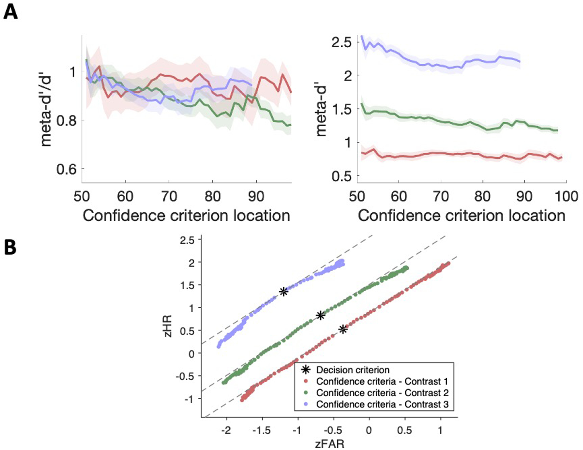
(A) Relationship between metacognitive scores and confidence criteria for meta-d’/d’ and meta-d’ after excluding criteria with >5% chance of producing 0 false alarms. Negative linear relationships can still be seen though the effect sizes are attenuated. The shaded areas represent across-subject S.E.M. (B) Empirical zROC functions with the same exclusion criteria. Again, the overall concave shape of the zROC curves is preserved but attenuated. For all zROC plots, the linear functions predicted by standard SDT are plotted as dashed grey lines for comparison and the (zFAR, zHR) pair generated by the decision criterion is marked as ‘*’.

Constructing a model of metacognitive inefficiency

Based on our empirical observations, we sought to build a process model of confidence generation that meets several criteria. First, the model should provide a better fit to the raw data than competing models. Second, the model should predict both the observed pattern of dependence of existing measures on the confidence criterion level and the shape of the empirical zROC curves. Third, the model should have an explicit connection to measuring metacognition; in other words, the process model should postulate the nature of metacognitive inefficiency and its parameters should then serve as theoretically-inspired measure of metacognitive ability. Finally, the measure of metacognitive ability implied by the model should be independent of both the confidence criterion and task difficulty.

A process model that meets the above criteria has to postulate an imperfect confidence generation process unlike standard models such as SDT (Figure 6). Such imperfection has typically been incorporated via the assumption of Gaussian metacognitive noise, that is, additional Gaussian noise corrupting the confidence ratings but not to the perceptual decision (Bang et al., 2019; De Martino et al., 2013; Fleming & Daw, 2017; Maniscalco & Lau, 2016; Mueller et al., 2008; Rahnev et al., 2016; Shekhar & Rahnev, 2018; van den Berg et al., 2017).

Figure 6. Computational models of confidence generation.

Depiction of three models of confidence generation: Standard SDT, Gaussian meta noise, and Lognormal meta noise. The three models are identical in postulating Gaussian sensory distributions for each stimulus category. At the metacognitive level, the models differ in how they generate confidence ratings. The Standard SDT model assumes a noiseless confidence generation process with the placement of deterministic confidence criteria on the evidence axis. The Gaussian and Lognormal meta noise models incorporate additional metacognitive noise (that is independent of sensory noise) into the confidence response. Metacognitive noise in these models refers to the trial-by-trial variability of the confidence criteria. The Gaussian and Lognormal meta noise models differ only in their assumptions about the distributional properties of the metacognitive noise. Note that alternative versions of the Gaussian and Lognormal meta noise model with variability in the sensory signal produce very similar results (Supplementary Analysis 6).

Models with Gaussian metacognitive noise, however, face at least two challenges. First, because the metacognitive noise is conceptualized as independent of the sensory noise, these models predict the existence of arguably nonsensical scenarios where on some trials the decision-level evidence points to one stimulus category but the meta-level evidence points to the other stimulus category (sometimes with high degree of confidence). Second, these models postulate the same level of noise for all confidence criteria, which runs counter to our findings that metacognition becomes more unreliable for higher confidence criteria.

To address these challenges, we created a model where metacognitive noise follows a lognormal distribution (Figure 6). The lognormal distribution, LN(μ, σ²), is defined on the interval (0,∞). Therefore, by defining the decision criterion as the zero of the evidence axis, we ensure that the resulting “Lognormal meta noise model” does not produce nonsensical scenarios where the decision and confidence conflict with each other. Further, for a given noise level, σ², criterion locations farther from the decision criterion feature higher variability. Thus, the Lognormal meta noise model appears to address both challenges faced by the Gaussian meta noise model.

The Lognormal meta noise model fits the data better than competing models

To formally evaluate the performance of our Lognormal meta noise model, we compared its ability to fit the raw data to two competing models: the Standard SDT model and the Gaussian meta noise model (Figure 6). For the purposes of model fitting, we transformed the continuous confidence scale into a 6-point scale, which required the estimation of 10 confidence criteria (5 criteria for each of the two stimulus categories) for every model. To evaluate the models’ performance, we compared the Akaike Information Criterion (AIC*) values generated by each model’s fit. AIC* measures the quality of models’ fits to the data while punishing the models for the number of free parameters.

AIC* analyses favored the Lognormal meta noise model over the Standard STD model by an average of 29.75 points (Figure 7 and Supplementary Table 1). The Lognormal meta noise model also outperformed the Gaussian meta noise model by an average AIC* of 17.46 points. We further corroborated these results by fitting the three models to Experiments 1, 3a, and 3b and demonstrating that the Lognormal meta noise model outperforms all other models though the differences were smaller due to the smaller amount of data per subject (Supplementary Tables 3, 4 & 5).

Figure 7. Model fitting results.

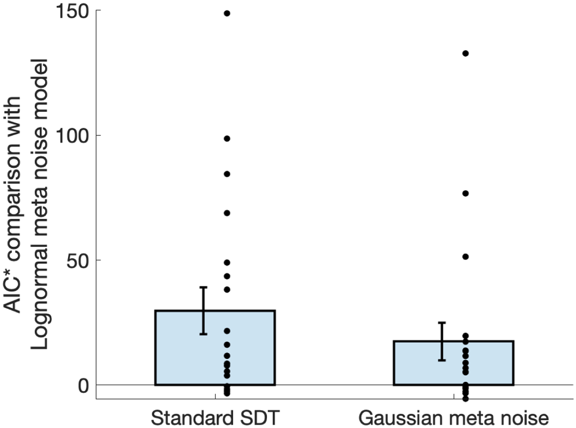
The Lognormal meta noise model significantly outperformed both the Standard SDT and the Gaussian meta noise models. Positive Akaike Information Criterion (AIC*) values indicate that the Lognormal meta noise model provided better fits to the data. Error bars indicate S.E.M. and dots indicate individual subjects.

However, close inspection of Figure 7 suggests the existence of a large variability between subjects: although the Lognormal meta noise model strongly outperformed the Standard SDT and the Gaussian meta noise models for some subjects, there was little difference between the models for others. If the Lognormal meta noise model provides a valid description of the confidence generation process for all subjects, then one may expect that the variability in the relative quality of model fits between models depends on subjects’ metacognitive performance. Indeed, high metacognitive performance would imply the existence of negligible metacognitive noise and thus all three models could be expected to fit equally well. On the other hand, low metacognitive performance would imply the existence of sizeable metacognitive noise, which, if described well by a lognormal distribution, would make the Lognormal model substantially outperform both the Standard SDT and Gaussian meta noise models.

We tested for this relationship by correlating the difference in AIC* values between the Lognormal meta noise model and its competing models with metacognitive performance as quantified by meta-d’/d’ (Figure 8). We found that the difference in AIC* between the Lognormal meta noise model and the Standard SDT model was very strongly correlated with meta-d’/d’ (r = .88, p = 3.7*10⁻⁷). This result is expected since lower metacognitive scores imply greater metacognitive noise, which can, in turn, be better accommodated by the Lognormal meta noise model to provide better fits to the data. However, the AIC* difference between the Lognormal and Gaussian meta noise models was also significantly correlated with meta-d’/d’ (r = .6, p = .005), which strongly supports the notion that metacognitive noise has a lognormal (or similar to lognormal) distribution. To further confirm the robustness of this relationship, we excluded one subject who showed a large difference in AIC* between the lognormal meta noise model and its competing models (ΔAIC* for Standard SDT: 148.8 and ΔAIC* for Gaussian meta noise model: 132.8). Recomputing the correlations between meta-d’/d’ and the AIC* difference, we found that the correlations decreased only slightly (Standard SDT: r changed from 0.88 to 0.87; Gaussian meta noise model: r changed from 0.62 to 0.46) with both correlations remaining significant (SDT: p = 9.7 * 10⁻⁷; Gaussian meta noise model: p = .0.047).

Figure 8. Relationship between metacognitive performance and the quality of model fits.

Correlation between meta-d’/d’ and the AIC* difference between the Lognormal meta noise model and both Standard SDT and Gaussian meta noise model. The difference in AIC* between the Lognormal meta noise model and its competing models increased as metacognitive performance (quantified by meta-d’/d’) decreased. These results suggest that the Lognormal meta noise model specifically outperforms other models when metacognition is imperfect. The grey lines represent the linear fits to the data. Circles depict individual subjects.

Only the Lognormal meta noise model accurately captures the relationship between measures of metacognition and the confidence criterion

Our empirical results established that metacognitive performance – as quantified by meta-d’/d’, meta-d’, Type-2 AUC, and Phi – depends on the confidence criterion location. Here we tested whether the three models above – the Lognormal meta noise, Gaussian meta noise, and Standard SDT – can predict the observed dependence of different measures of metacognition on the confidence criterion. Following our analyses of the empirical data, we quantified the relationship between the measures and confidence criteria by fitting linear functions (for meta-d’/d’ and meta-d’) and quadratic functions (for Type-2 AUC and Phi) to individual-subject data for each level of contrast. For the linear fits, we tested the significance of the estimated slopes; for the quadratic fits, we tested estimates of the parameter controlling the curvature of the parabola.

We observed a stark difference between the three models in their predictions about the relationship between the confidence criterion level and the measures meta-d’/d’ and meta-d’ (Figure 9; average parameter estimates, as well as t and p values are reported in Supplementary Table 7). Only the Lognormal meta noise model successfully captured the fact that both of these measures decreased with increasing confidence criterion in the empirical data (Figure 3). Indeed, the Lognormal meta noise model predicted negative slopes for both meta-d’/d’ and meta-d’ for each of the three contrasts (p < .0001 for all six slopes). On the other hand, the Standard SDT model predicted that meta-d’/d’ and meta-d’ both remain constant for increasing confidence criteria (p > .35 for all six slopes). This is unsurprising because meta-d’ is designed within the SDT framework and in the absence of any corrupting influence on confidence, it should always be equal to d’ for all criterion levels. Finally, the Gaussian meta noise model predicted that both meta-d’/d’ and meta-d’ would increase with increasing confidence criterion (p < .006 for all six slopes). In other words, the Gaussian meta noise model makes a qualitatively wrong prediction about how meta-d’/d’ and meta-d’ depend on confidence level.

Figure 9. Predictions of Standard SDT, Gaussian meta noise, and Lognormal meta noise models for the dependence of existing measures of metacognition on the confidence criterion.

We observed a stark difference in the models’ predictions for the relationship between confidence criteria and the measures meta-d’/d’ and meta-d’. While the Lognormal noise model successfully captured the empirically observed negative relationship between metacognition and confidence criterion for meta-d’/d’ and meta-d’, the Gaussian meta noise and Standard SDT models predicted qualitatively different relationships between metacognitive scores and confidence criteria for these measures. For the other two measures, Type-2 AUC and Phi, all the three models consistently predicted an inverted U-shaped function, suggesting that the strong parametric assumptions of these measures overshadowed the effect of metacognitive noise. The shaded areas represent the S.E.M. of the measures across subjects.

Despite the large differences between the three models in their predictions about meta-d’/d’ and meta-d’, there was a remarkable agreement between them in regards to both Type-2 AUC and Phi (Figure 9). Specifically, all three models correctly predicted the inverted U-shape functions observed for these measures in the empirical data (all p’s < .0001). These results suggest that the parametric assumptions of both Type-2 AUC and Phi are so strong that they can be captured with any SDT-based model regardless of whether the model even postulates the presence of metacognitive inefficiency.

Only the Lognormal meta noise model accurately captures the observed zROC curves

Our experimental data revealed that zROC functions are robustly nonlinear (Figure 4). Here we tested whether the three models above – the Lognormal meta noise, Gaussian meta noise, and Standard SDT – can predict the observed zROC shapes. From our previous simulations of the confidence generation process, we estimated the zROC functions separately for each subject and contrast level. We plotted the average zROC function within each contrast level by averaging across all subjects. (Figure 10). As in the empirical data, we quantified the overall curvature of zROC functions predicted by each model by fitting a quadratic function for each individual subject and for each level of contrast. Quadratic coefficients a < 0 indicate zROC functions with an overall downward curvature.

Figure 10. Predictions of Standard SDT, Gaussian meta noise, and Lognormal meta noise models for the observed zROC functions.

Standard SDT predicted linear zROC functions for all contrasts. On the other hand, both the Gaussian and Lognormal meta noise models predicted zROC functions with downward curvature, as observed in our empirical data (Figure 4). However, only the Lognormal meta noise model captured the overall level of concaveness, with the Gaussian meta noise model significantly underestimating the overall concaveness.

We observed that only the Lognormal meta noise model was able to quantitatively capture the overall concaveness of the zROC curves. Indeed, the estimated quadratic coefficient a for the Lognormal meta noise model was significantly negative for each level of contrast (Contrast 1: Mean = −0.018, t(19) = −4.24, p = 0.0004; Contrast 2: Mean = −0.031, t(19) = −4.12, p = 0.0005; Contrast 3: Mean = −0.050, t(19) = −4.45, p = 0.0003), and, more importantly, was not significantly different from those obtained from the quadratic fits to empirical zROC curves (Contrast 1: Mean difference = .005, t(19) = 1.53, p = .14; Contrast 2: Mean difference = −0.009, t(19) = −1.35, p = 0.20; Contrast 3: Mean difference = −0.01, t(19) = −0.84, p = 0.40). On the other hand, the curve fits for the Gaussian model also yielded significantly negative estimates of the quadratic coefficient a for contrasts 1 and 2 (Contrast 1: Mean = −0.002, t(19) = −2.15, p = 0.008; Contrast 2: Mean = −0.04, t(19) = −2.46, p = 0.02; Contrast 3: Mean = −0.004, t(19) = −1.73, p = 0.09), but these estimates were significantly smaller than the empirically-observed values for contrasts 2 and 3 and marginally smaller for contrast 1 (Contrast 1: Mean difference = −.01, t(19) = −1.93, p = 0.07; Contrast 2: Mean difference = −0.034, t(19) = −4.25, p = 0.0004; Contrast 3: Mean difference = −0.05, t(19) = −4.34, p = 0.0003). Finally, the Standard SDT model predicted estimates of the quadratic coefficient a that were not significantly different from zero (Contrast 1: Mean = −0.0009, t(19) = −0.8, p = 0.43; Contrast 2: Mean = −0.001, t(19) = −0.68, p = 0.50; Contrast 3: Mean = −0.003, t(19) = −1.01, p = 0.32) and were significantly smaller than the empirically-observed values (Contrast 1: Mean difference = −.01, t(19) = −2.32, p = 0.03; Contrast 2: Mean difference = −0.04, t(19) = −4.57, p = 0.0002; Contrast 3: Mean difference = −0.05, t(19) = −4.54, p = 0.0002), as expected given that SDT is known to imply linear zROC functions (Green & Swets, 1966).

In addition, both the Gaussian and the Lognormal meta noise models predicted zROC functions with increasing curvature for increasing contrast levels, as observed in the empirical zROC plots. Indeed, the one-way repeated measures ANOVAs on the quadratic coefficient a revealed significant mean differences between the zROC functions for the three contrast levels for both models (Lognormal model: F(2,19) = 20.65, p = 8.5 × 10⁻⁷; Gaussian model: F(2,19) = 8.12, p = 0.001). Pairwise comparisons confirmed that the quadratic coefficient a increased significantly for higher levels of contrast for all possible comparisons for both models (all p’s < 0.014). Thus, both models qualitatively capture the empirically-observed increased overall curvature of zROC functions for higher contrasts though the Lognormal meta noise model provides more precise quantitative fits.

The Lognormal meta noise model leads to a measure of metacognition that is independent of the confidence criterion

Our empirical results demonstrated that metacognitive performance depends on the level of confidence. However, researchers are typically interested not in the level of performance in a specific condition but in the overall ability of the subject. (For example, d’ is typically preferred over percent correct exactly because it does not change as bias increases even though higher bias means that the subject is answering correctly less frequently.) Therefore, a measure of the true metacognitive ability of a person should not depend on the level of confidence and must reflect only those changes that affect metacognitive processing itself. Our results suggest that no existing measure meets this criterion.

We therefore tested whether the estimated metacognitive noise, σ_meta, in our Lognormal meta noise model could serve as a measure of metacognitive ability that is uncontaminated by the confidence level or the performance of the subject on the primary task. We ran the model fitting procedure independently for each of the five confidence criteria (that were previously defined for transforming our continuous confidence data into 6-point ratings for the main fitting procedure; see Methods for details) and for each of the three contrast levels. From this fitting procedure, we obtained independent estimates of σ_meta for each level of the confidence criterion as well as for each level of contrast.

We first assessed the main effects of confidence criterion location and stimulus contrast on σ_meta from each model by performing two-way ANOVAs. We found that σ_meta, as computed based on the Lognormal meta noise model, was insensitive to both confidence criterion location and contrast. Indeed, a two-way ANOVA revealed no main effect of confidence criterion (F(4,19) = 1.21, p = .31) or stimulus contrast (F(2,19) = .66, p = .52) on σ_meta estimated from the Lognormal meta noise model (Figure 11A). On the other hand, we found that σ_meta estimated from the Gaussian meta noise model increased significantly for higher confidence criterion locations (F(4,19) = 8.95, p = 5.6 × 10⁻⁵; Figure 11B) but did not vary with stimulus contrast (F(2,19) = .89, p = .42). For both models, the interaction between stimulus contrast and confidence criterion was not significant (Lognormal meta noise model: F(2,4) = 1.38, p = 0.21, Gaussian meta noise model: F(2,4) = 1.77, p = 0.09) indicating that the relationship between σ_meta and confidence criterion is similar across contrasts.

Figure 11. Dependence of the estimated metacognitive noise parameter σ_meta on confidence criterion for the Lognormal and Gaussian meta noise models.

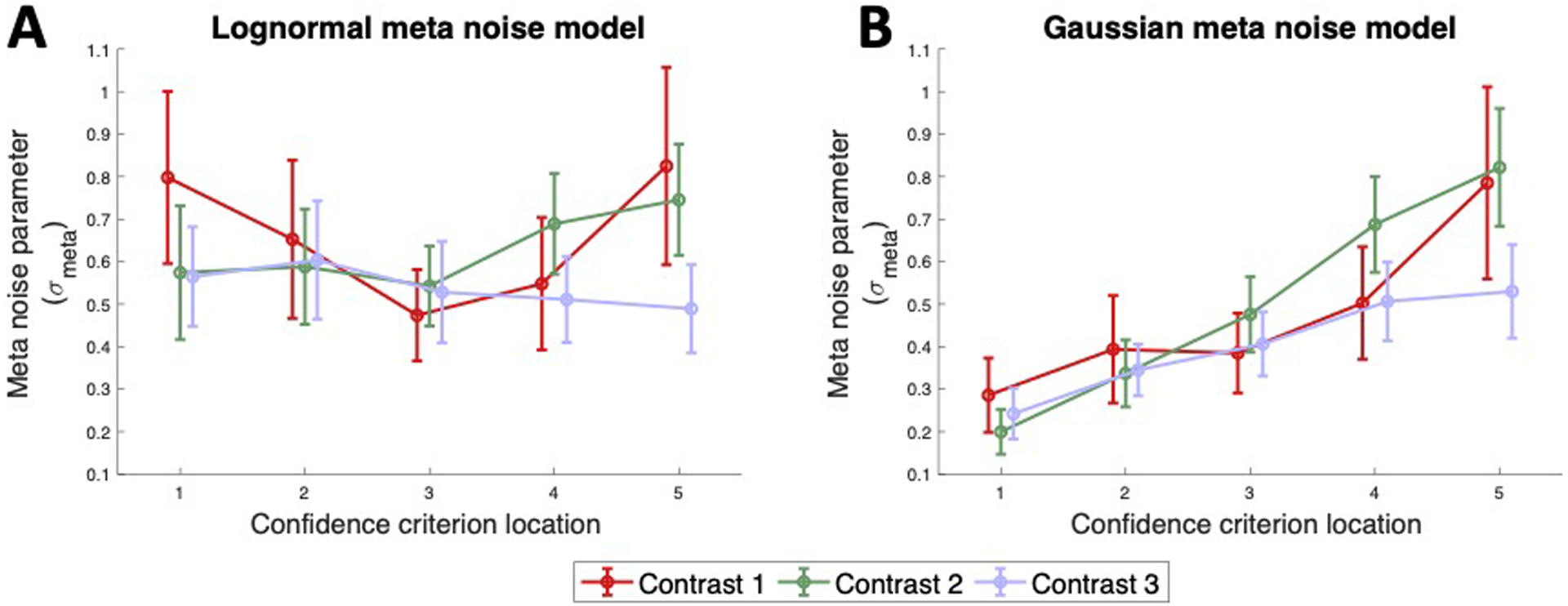
(A) The estimated metacognitive noise σ_meta from the Lognormal meta noise model remains constant for different confidence criterion locations and contrasts. (B) The estimated metacognitive noise σ_meta from the Gaussian meta noise model increase with confidence criterion location but is independent of contrast. Thus, metacognitive noise derived from the Lognormal meta noise model but not from the Gaussian meta noise model could be used as a more robust measure of true metacognitive ability. Error bars indicate S.E.M.

To further corroborate this conclusion, we ran Bayesian statistical analyses that can quantify the evidence in favor of our null hypothesis that σ_meta is unaffected by confidence criterion and stimulus contrast. In these analyses, we computed the Bayes Factor (BF) which measures evidence in favor of the null hypothesis (no main effects of contrast, confidence criterion, or the interaction between the two) relative to evidence in favor of alternative hypotheses which include these effects. In the case where σ_meta was derived from the Lognormal meta noise model, we found that the null model was favored over all alternative models (model with main effect of contrast only: BF₀₁ = 13.42; model with main effect of criterion location only: BF₀₁ = 94.79; model with effects of both contrast and criterion location: BF₀₁ = 1.4 × 10³; model with effects of contrast, criterion location, and interaction between them: BF₀₁ = 2.5 × 10⁵). On the other hand, when σ_meta was derived from the Gaussian meta noise model, the best model included a simple main effect of confidence criterion (BF₁₀ = 1.2 × 10⁷). These findings provide strong support for the notion that σ_meta derived from the Lognormal meta noise model (but not when derived from the Gaussian meta noise model) is independent of both difficulty and confidence criterion location and thus could be used as a more robust measure of true metacognitive ability.

Discussion

We found that metacognitive performance depends on confidence level. This finding was robust across five previous and one new datasets and four measures of metacognitive ability. Further, we showed that empirical zROC functions constructed from confidence ratings, widely believed to be linear, have a distinctly concave overall shape. Based on these findings, we developed a process model of metacognition, which assumes that confidence criteria are drawn from a lognormal distribution. The resulting Lognormal meta noise model significantly outperformed competing models with deterministic confidence criteria (Standard SDT model) or with confidence criteria drawn from Gaussian distributions (Gaussian meta noise model). Finally, we showed that the Lognormal meta noise model was able to yield a measure of metacognition, σ_meta, that is independent of confidence levels. Our findings uncover a new mechanism underlying metacognitive inefficiency, derive an empirically-validated process model of confidence generation, and carry important implications for measuring metacognition.

Joint development of process models of confidence generation and measures of metacognition

Process models of metacognition are intricately tied to measures that quantify metacognitive ability. Specifically, a model that proposes a specific mechanism for a given process should generate a measure in the form of a parameter (or a combination of parameters) that is sensitive only to changes in that process. Conversely, all measures of metacognitive ability implicitly assume a process model that generates them. Therefore, assessing the sensitivity of metacognitive measures to nuisance variables can allow us to test the validity of their implicit process models. If we find that a measure depends on one or more nuisance variables, this would imply that its associated process model is either unable to effectively tease apart metacognitive processes from other extraneous influences or is failing to capture metacognitive processes in their entirety.

However, this strong link between process models of confidence generation and measures of metacognition has remained largely unrecognized. Consequently, no current process model of metacognition has been used to create a measure of metacognition, and no existing measure of metacognition has been linked to its implied process model of confidence generation. Our Lognormal meta noise model provides the first explicit bridge between models of confidence generation and measures of metacognition. Future work on either process models of confidence or on measures of metacognition should attempt to connect explicitly these two areas of research.

The concept of metacognitive noise

The existence of metacognitive noise is at the heart of our Lognormal meta noise model. Several studies have previously postulated the existence of metacognitive noise to explain metacognitive inefficiency. Bang et al. (2019) demonstrated that models with metacognitive noise make the unique prediction that sensory noise would increase metacognitive efficiency and confirmed the prediction in three different experiments. Further, models with metacognitive noise explained observed accuracy-confidence dissociations better than dual-channel models (Maniscalco and Lau, 2016) and captured the effects of transcranial magnetic stimulation to different sites in the prefrontal cortex (Shekhar & Rahnev, 2018). The existence of metacognitive noise has also received support in memory literature with the finding that its inclusion in models generates significantly better fits to the data (van den Berg et al., 2017).

Nevertheless, the exact source of this metacognitive noise remains unclear. Metacognitive noise is an umbrella term encompassing all noise sources that selectively influence the confidence generation process. Mounting evidence suggests that confidence generation incorporates many types of non-perceptual information that have little to no influence on the perceptual decision. For example, confidence ratings are influenced by previous confidence ratings (Rahnev et al., 2015), arousal (Allen et al., 2016), and action fluency (Fleming et al., 2015). Further, metacognitive decisions have been suggested to use a heuristic strategy that ignores evidence against a perceptual choice (Maniscalco et al., 2016; Peters et al., 2017; Zawadzka, Higham, & Hanczakowski, 2017). Fatigue (Maniscalco, McCurdy, Odegaard, & Lau, 2017) and working memory manipulations (Maniscalco & Lau, 2015) can also selectively impact metacognitive judgements. Finally, metacognitive but not perceptual sensitivity can be perturbed by transcranial magnetic stimulation (Rahnev et al., 2016; Rounis et al., 2010; Ryals, Rogers, Gross, Polnaszek, & Voss, 2016; Shekhar & Rahnev, 2018) and lesions (Fleming, Ryu, Golfinos, & Blackmon, 2014) to the prefrontal cortex. Collectively, these studies demonstrate a set of factors which selectively influence metacognition and may serve as plausible sources of metacognitive noise.

Adding metacognitive noise to the confidence criteria vs. the perceptual signal

Here we modeled metacognitive noise as variability of the confidence criterion but previously we modeled metacognitive noise as affecting the perceptual signal at the metacognitive stage (Bang et al., 2019; Shekhar & Rahnev, 2018). In the absence of additional manipulations, these two ways of modeling metacognitive noise are equivalent for the Gaussian meta noise model (see Supplementary Analysis 6 for a demonstration of this equivalence). These two implementations are not mathematically equivalent for the Lognormal meta noise model but additional model fitting analyses showed that they produce virtually the same results (Supplementary Analysis 6 and Supplementary Table 8).

Nevertheless, conceptually, noise in the perceptual signal and noise in the confidence criteria correspond to different sources of inefficiency in the system: noise could come from poor information transmission to areas responsible for confidence generation (conceptually captured by noise added to the signal) or poor confidence generation (conceptually captured by noise added to the criterion). We suspect that both of these sources of noise contribute non-trivially to the overall metacognitive noise. Teasing these influences apart is an important topic for future research.

The distributional properties of metacognitive noise

Our results strongly suggest that metacognitive noise is better described by a lognormal rather than a Gaussian distribution. The distributional properties of metacognitive noise have not been previously examined and researchers have typically assumed, as default, a Gaussian distribution. However, Gaussian metacognitive noise leads to nonsensical situations where the sensory evidence on the decision level points to one stimulus category but the metacognitive level dictates a rating of high confidence for the other stimulus category. Gaussian metacognitive noise also cannot account for our observation that metacognitive inefficiency increases with higher confidence criteria. Modeling metacognitive noise with a lognormal distribution, which has a lower bound and whose variance scales with its mean, addresses both of these limitations.

Why may metacognitive inefficiency follow a lognormal distribution? It has long been established that cortical neurons exhibit a fairly stable normalized variability (quantified as the Fano Factor, which is equal to variance divided by the mean). In other words, higher firing rates lead to higher variability of the across-trial neuronal response (Dean, 1981; Tolhurst, Movshon, & Dean, 1983; Tolhurst, Movshon, & Thompson, 1981). It is likely that neural implementations of high confidence criteria or high sensory signal may entail increased firing rates and that these increased firing rates would then be expected to be more variable from trial to trial. This mechanism may explain why metacognitive variability increases with confidence criteria. The idea that noise levels increase for higher values of the sensory evidence has received substantial support in the context of research on attention and visual perceptual learning (Dosher & Lu, 1999, 2017; Lu & Dosher, 2008; Lu et al., 2002). This research has demonstrated the presence of signal-dependent multiplicative noise. This type of noise is very similar to our use of a lognormal distribution for modeling the noise in confidence criteria although this previous work did not explore the implications of multiplicative noise to models of metacognition. Finally, the notion that confidence representations are derived from logarithmic mapping of evidence has also been previously explored by van den Berg et al. (2017). In their generative model, confidence responses were computed as logarithmic transformation of evidence (measured as memory precision) followed by the addition of normally distributed metacognitive noise. This computation is equivalent to adding lognormal metacognitive noise to the evidence variable before the log transformation.

Another potential explanation for these patterns of results may come from probability distortions which lead to increasing over- or underestimation of probability for higher probability estimates. However, probability distortions are unlikely to cause variations in metacognitive accuracy because they are typically associated with systematic biases in confidence. As long as these shifts are consistent (occurring in one particular direction) for a given level of confidence, they should not lead to changes in metacognitive ability. We confirmed these expectations by simulating the effects of probability distortions in a standard SDT model (as described by Zhang and Maloney, 2012). We found that probability distortion consistently led to either over- or underestimation of confidence, because the confidence criteria are shifted either inwards or outwards. However, the probability distortion had no significant effect on metacognitive scores (Supplementary Figure 8).

Finally, it is important to clarify that we do not claim that the structure of metacognitive noise is exactly lognormal. The general phenomenon of metacognition becoming more imperfect with high confidence criteria can be captured by a number of distributions whose variance scales with their mean – such as Gamma or chi-squared distributions. Future work should explore whether any other distribution provides an even better description of the data.

zROC functions in perceptual decision making

A substantial amount of research has demonstrated the existence of nonlinear zROC functions in memory research (Ratcliff et al., 1994; Ratcliff & Starns, 2013; Voskuilen & Ratcliff, 2016; Yonelinas, 1999; Yonelinas & Parks, 2007). However, empirical zROC functions have not received much scrutiny in perceptual decision making. Using confidence ratings collected on a continuous scale, we smoothly varied the confidence criterion and plotted zROC functions with high resolution. Our results revealed the existence of robustly nonlinear zROC curves in perceptual decision making.

Further, we observed that the curvature of zROC functions increases with higher stimulus contrast levels. This effect was nicely captured by our Lognormal meta noise model even though the model was not explicitly designed to do so. Why does the Lognormal meta noise model predict different zROC curvatures for different contrasts? To clarify this, it is helpful to first explore why the Lognormal meta noise model predicts any curvature at all. The model postulates the existence of larger noise in the extreme confidence criteria. Critically, large noise in the extreme confidence criteria to the right of the decision criterion has larger impact on zHR than zFAR because these criteria have a larger overlap with the target compared to the non-target distribution. Equivalently, large noise in the extreme confidence criteria to the left of the decision criterion has larger impact on zFAR than zHR. Together, these effects create the curvature in zROC functions predicted the Lognormal meta noise model. Once this effect is appreciated, it becomes clear that the curvature can be expected to be relatively small when the target and non-target distributions are relatively close to each other (as is the case for low contrasts) and increase as the target and non-target distributions diverge more (as is the case for high contrasts).

Nevertheless, it should be noted that even though the Lognormal meta noise model is successful in capturing the overall curvature of the zROC functions, it does not capture the shape of the empirical zROC functions precisely. Specifically, rather than a function with smooth downwards curvature, the Lognormal meta noise model predicts functions which appear to be piecewise linear and decreasing on both side of the decision criterion. It is thus possible that models where metacognitive noise follows other functions (e.g., Gamma or chi-squared distributions) would provide a better fit. Nevertheless, the Lognormal meta noise model is more successful than existing competing models in quantitatively capturing the global trend of the zROC curvature.

An important question that arises from these findings is whether other models or theories can explain the observed concave zROC functions. Both concave and convex zROC functions have been observed in recognition memory and have been modeled as arising from a dual processes of recognition and familiarity (Yonelinas, 1999). Such models, however, are pertinent only to memory and cannot be easily extended to perceptual decision making. The only other model that has been used to explain nonlinear zROC functions is the Response-Time Confidence (RTCON) model (Ratcliff & Starns, 2009; Voskuilen & Ratcliff, 2016) in which confidence is the outcome of competing evidence accumulators, each representing one possible confidence response. In RTCON, the threshold for each confidence accumulator is set independently and varying these thresholds in relation to each other can lead to various zROC shapes. For example, when the thresholds are more liberal for extreme confidence criteria, zROC functions are concave, whereas the opposite pattern results in convex zROCs. Thus, RTCON can account for any zROC shape but does not predict a priori whether convex or concave zROC functions should be observed in perceptual decision making. In contrast, our Lognormal meta noise model is considerably more constrained and offers a plausible mechanistic explanation for the concave zROC curves in perceptual decision making.

Finally, it is currently unclear whether other existing models such as dual-channel models (Del Cul, Dehaene, Reyes, Bravo, & Slachevsky, 2009; Maniscalco & Lau, 2016), second-order Bayesian inference models (Fleming & Daw, 2017), or models developed to account for reaction times (Kiani, Corthell, & Shadlen, 2014; Moran, Teodorescu, & Usher, 2015; Pleskac & Busemeyer, 2010; Vickers, 1979) can explain concave zROC functions. We note that none of these previous models include mechanisms where higher confidence ratings become less reliable but further research is needed to establish whether these models may be able to predict zROC functions with a downward curvature.

Implications for measuring metacognition

Our results demonstrate that all popular measures of metacognition are significantly affected by confidence bias. Specifically, meta-d’ and meta-d’/d’ decreased with higher confidence criteria, whereas Phi and Type-2 AUC followed an inverted U-shape function. Therefore, subjects who have a bias towards low confidence (and are thus using high confidence criteria) may be wrongly inferred to have lower metacognitive ability when that ability is quantified using meta-d’ or meta-d’/d’. Similarly, subjects with very high or very low confidence may be wrongly inferred to have lower metacognitive ability when that ability is quantified using Phi or Type-2 AUC. Therefore, when metacognitive ability is compared, researchers should attempt to match confidence levels between groups of subjects or conditions. Further, the results of experiments with very few confidence ratings (especially binary confidence scales) may be more prone contamination by the confidence level of the subject. Using confidence scales with multiple levels should make the results more robust to confidence biases because the confidence criteria used by the subject are likely to cover a larger part of the confidence scale.

Our results demonstrate that the lognormal metacognitive noise parameter σ_meta does not vary with task difficulty. Therefore, σ_meta can be used as a measure of metacognitive efficiency, that is a measure of metacognition that does not vary with task difficulty (Fleming & Lau, 2014). Further, unlike all existing measures of metacognition, σ_meta is invariant to changes in confidence criterion, thus suggesting that it may potentially be a better measure of metacognitive efficiency than existing ones. However, any principled measure of metacognition must also be insensitive to variation in response bias. Since we did not experimentally manipulate response bias in our current study, we cannot yet inform the question of whether our proposed measure is indeed robust to changes in response bias. It will also be important to test how stable the parameter σ_meta is in common situations where relatively limited data are available. Therefore, before metacognitive noise can be accepted as a valid measure of metacognitive efficiency, additional tests are required to fully establish its properties.

Predictions of the Lognormal meta noise model

Any good model should not only fit existing data but should also ideally make new predictions. Our Lognormal meta noise model makes a clear prediction that can be tested empirically. Specifically, the model predicts that a bias towards low confidence must be associated with lower meta-d’ and meta-d’/d’ even when subjects use confidence scale with multiple confidence ratings. In our current study, a similar dependence was demonstrated by analytically manipulating the confidence scale within the same subjects. However, this prediction also holds between different subjects such that there should be a positive across-subject correlation between average confidence and both meta-d’ and meta-d’/d’.

Limitations of the Lognormal meta noise model

The Lognormal meta noise has several desirable features: it (i) captures the dependence of meta-d’ and meta-d’/d’ on confidence criterion, (ii) explains the concave shape of zROC functions in perceptual decision making, and (iii) provides the first link between process models of confidence generation and measures of metacognitive ability.

However, the model also has several limitations. First, the Lognormal meta noise model cannot be used to model RT unlike models based on sequential sampling. Second, our model cannot inform theories of post-decisional evidence processing because it is equivocal about the timing of confidence decisions with respect to the choice. Indeed, although the Lognormal meta noise model posits that independent noise sources underlie perceptual and confidence decisions, it does not commit to the interpretation that this independence necessarily arises from post-decisional processing. Third, the model does not specify the exact sources of metacognitive noise but simply specifies the distribution of the noise resulting of all corrupting influences considered together. Thus, the Lognormal meta noise model does not directly relate to previous work on either RT or post-decision evidence accumulation, and does not allow for direct identification of specific sources of metacognitive noise.

Another limitation of the Lognormal meta noise model is that it cannot account for error detection or changes of mind since the confidence rating is constrained to never contradict the original decision. We note that the Gaussian meta noise model leads to situations where the perceptual decision and the confidence rating disagree. However, in that model, the perceptual decision is more reliable than the confidence rating, which is the opposite effect of what is observed in changes of mind where subjects are more likely to correct a wrong decision into a correct one (Resulaj et al., 2009). We further note that the recently proposed second-order model by Fleming and Daw (2017), which readily accounts for changes of mind, can, in fact, subsume the Gaussian meta noise model. More specifically, the two models become similar when the noise in the decision variable in the second-order model by Fleming and Daw is lower than the noise in the confidence variable and the correlation between the two variables is high.

A final limitation of the Lognormal meta noise model is that it cannot accommodate findings of meta-d’/d’ > 1. We note, however, that such findings are controversial because most demonstrations have come from studies that use continuous staircase paradigms and we have recently demonstrated that mixing different difficulty levels in this way leads to a strong overestimation of metacognitive scores including meta-d’/d’ (Rahnev & Fleming, 2019). Therefore, it is still unclear whether meta-d’ can be truly greater than d’. We also note that it is possible to extend the Lognormal meta noise model to account for meta-d’/d’ > 1 by adding either a lapse rate parameter or late decision noise.

Conclusion

We demonstrated a robust dependence between current popular measures of metacognition and confidence levels. Nonlinearities in empirical zROC functions confirmed not only the existence of metacognitive noise but also that this noise increases for higher confidence criteria. To account for these empirical insights, we developed a new process model of metacognition that successfully yielded a measure of metacognition that was stable across confidence and contrast levels. Our results carry important implications for measuring metacognition while revealing the nature of the inefficiencies underlying the process of confidence generation.