SAMPLING OF SURFACES AND LEARNING FUNCTIONS IN HIGH DIMENSIONS

Abstract

The efficient representation of data in high-dimensional spaces is a key problem in several machine learning tasks. To capture the non-linear structure of the data, we model the data as points living on a smooth surface. We model the surface as the zero level-set of a bandlimited function. We show that this representation allows a non-linear lifting of the surface model, which will map the points to a low-dimensional subspace. This mapping between surfaces and the well-understood subspace model allows us to introduce novel algorithms (a) to recover the surface from few of its samples and (b) to learn a multidimensional bandlimited function from training data. The utility of these algorithms is introduced in practical applications including image denoising.

1. INTRODUCTION

The learning and exploitation of the structure in real-world multidimensional datasets is a key problem in machine learning. Classical solutions to these problems often rely on linear or sparsity-based schemes [1]. Deep-learning based algorithms are now emerging as powerful alternatives to these methods, offering significantly improved performance over the above approaches in representation [2] as well as learning tasks (e.g. denoising [3], classification [4]). Despite their popularity, the theoretical understanding of these frameworks is lacking. It is believed that the ability of these schemes to efficiently capture the non-linear manifold structure of data may be the reason for many of their desirable properties.

The main focus of this work is to introduce a novel signal model to capture the structure of high-dimensional datasets, which facilitates the development of theoretically tractable learning algorithms. Specifically, we model the training data samples as points on a union of smooth surfaces in high dimensional space. We model the surfaces as zero level-sets of a bandlimited function ψ. A more band-limited ψ will translate to a smoother surface; the bandwidth of ψ can be viewed as a measure of the complexity of the surface. We term such surfaces as bandlimited surfaces. This model allows us to introduce an exponential lifting operation, which maps the complex union of surfaces model to the well understood union of subspaces (UoS) representation [5]. Specifically, we show that an exponential lifting of the data living on a surface results in a low-dimensional feature subspace. We rely on the low-dimensional nature of the feature subspace for two applications: (a) recovery of surfaces in high dimensional spaces from its samples, and (b) efficient representation of high-dimensional functions from limited labeled training data, assuming that the training samples live on bandlimited surfaces.

In the surface recovery problem, we introduce an algorithm to recover the surface from noisy data points. The scheme estimates the null-space of the feature matrix of the measured points, which uniquely specifies the surface. We also introduce a sampling theory, which guarantees the recovery of the union of surfaces from its few samples. These results show that the surface can be uniquely identified with unit probability from noiseless samples, whenever the number of random samples on the surface exceed the degrees of freedom of the surface.

The subspace structure of the lifted data also facilitates the efficient computation of functions of the data points. Specifically, a bandlimited function of the data points can be expressed as the linear combination of exponential features. Note that exponential features live in a low-dimensional subspace, when the points are localized to a smooth surface. Hence, bandlimited functions of the data points can be efficiently computed using few basis functions in the feature space; our results show that such bandlimited functions can be evaluated as the Dirichlet interpolation of the a few function samples on the surface; the number of function samples (labeled data-sets) needed is significantly smaller than the degrees of freedom of the function, which facilitates a very compact representation. The significant reduction in the number of free parameters makes the learning of the function from finite samples tractable.

We show that the computational structure of the representation is essentially a one-layer kernel network, where the non-linearity is specified by a Dirichlet function. We note that the structure is similar to radial basis function (RBF) network [1, 6]. Unlike the RBF setting, the computation does not involve the evaluation of the function at all the available training data points, which is a key limitation of RBF networks. When the data is restricted to a bandlimited surface, we show that the computation only requires the evaluation of the function on a small number of anchor points on the surface, whose number is dependent on the smoothness or bandwidth of the surface. This approach thus justifies the use of sparse RBF networks with Dirichlet kernels.

This work builds upon our prior work [7, 8, 9], where we considered the recovery of planar curves from few of its samples. This work extends the above results in three important ways (i). the planar results in the above works are generalized to the high dimensional setting. (ii). the worst-case sampling conditions are replaced by high-probability results, which are far less conservative, and are in good agreement with experimental results. (iii). The sampling results are extended to the local representation of functions.

2. BACKGROUND

We model each surface as the zero level-set of the function ψ

$$\mathcal{Z}[\psi ]=\left\{\text{x}\in {ℝ}^n:\psi (\text{x})=0\right\}$$ (1)

where ψ is a bandlimited function, whose bandwidth is specified by the set Λ:

$$\psi (\text{x})=\sum _{\text{k}\in \Lambda }{\text{c}}_{\text{k}}\text{exp}\left(\text{j}2\pi {\text{k}}^T\text{x}\right),\text{x}\in {\left[0,1\right)}^n.$$ (2)

The cardinality of the set Λ, which is denoted by |Λ| is the number of free parameters in the surface representation, and can be viewed as a measure of the complexity of the union of surfaces $\mathcal{Z}[\psi ]$. We now consider an arbitrary point x on the zero-set $\mathcal{Z}[\psi ]$. Combining (1) and (2), we have

$$\sum _{k\in \Lambda }{\text{c}}_{\text{k}}\text{exp}\left(j2\pi {\text{k}}^T\text{x}\right)={\text{c}}^T{\Phi }_{\Lambda }(\text{x})=0.$$ (3)

Here, the nonlinear feature map ${\Phi }_{\Lambda }:{ℝ}^n\to {ℂ}^{\left|\Lambda \right|}$

$${\Phi }_{\Lambda }(\text{x})={\left[\text{exp}\left(j2\pi {\text{k}}_1^T\text{x}\right)\cdots \text{exp}\left(j2\pi {\text{k}}_{\left|\Lambda \right|}^T\text{x}\right)\right]}^T$$

lifts a point x ∈ [0, 1)ⁿ. Note that there are |Λ| features. The null-space relation c^TΦ_Λ(x) = 0 implies that c is orthogonal to the feature space of the points, which implies that the features live in a |Λ| − 1 dimensional space. Note that this non-linear lifting to feature spaces is similar to the one used in kernel methods [1]. In this work, we restricted our attention to bandlimited surfaces. However, the analysis may also be extended to other parametric level-set representations involving other basis functions [10].

3. SURFACE RECOVERY FROM SAMPLES

Assume that we have N samples on the surface, denoted by X = {x₁,·⋯ ,x_N}. Since all of these points satisfy (2), we have

$${\text{c}}^T\underset{{\Phi }_{\Lambda }(\text{X})}{\underbrace{\left[{\Phi }_{\Lambda }\left({\text{x}}_1\right)\cdots {\Phi }_{\Lambda }\left(x_N\right)\right]}}=0.$$ (4)

The above relation implies that the rank of the feature matrix Φ_Λ(X) is at most N − 1. One can use the above null-space relation to recover the coefficient vector c, and hence the surface, from the samples X. Note that there is a one-to-one correspondence (up to scaling) between the coefficient set and the surface. Hence, to uniquely determine the zero level-set of ψ(x), we require

$$\text{rank}\left({\Phi }_{\Lambda }(\text{X})\right)=\left|\Lambda \right|-1.$$ (5)

The following discussion tells us when the feature matrix satisfy this rank condition, and thus guarantees surface recovery.

3.1. Surface recovery from noisy-free samples

We first focus on the case that the samples are noisy-free. The results in this section can be viewed as the generalization of the recovery of subspaces or low-rank matrices from few samples to the surface setting. The following result show that an irreducible surface can be uniquely identified from its random samples when the number of samples exceed the degrees of freedom, denoted by |Λ| − 1.

Proposition 1:

Let $\mathcal{Z}[\psi ]$ be an irreducible surface with bandwidth Λ. Then, the surface can be uniquely recovered with probability one from its N random and independent samples, when N ≥ |Λ| − 1.

3.2. Recovery from noisy samples

In practice, the bandwidth of the surface Λ is unknown. A simple approach is to choose a large enough bandwidth Γ such that Λ ⊆ Γ. In this case we have the following result.

Proposition 2:

Consider an arbitrary set of points x₁, …, x_N living on the union of surfaces $\mathcal{Z}[\psi ]$ with the bandwidth of ψ being Λ. Then, the feature matrix Φ_Γ(X) with Γ ⊃ Λ satisfies

$$\text{rank}\left({\Phi }_{\Gamma }(\text{X})\right)=\left|\Gamma \right|-\left|\Gamma \ominus \Lambda \right|.$$ (6)

Here, Φ_Γ(X) is the feature matrix evaluated assuming the bandwidth to be Γ. The notation Γ ⊖ Λ is the set corresponding to all the valid shifts of Λ within Γ; it is obtained as the binary erosion of the set Γ by Λ.

These results imply that the feature matrix Φ_Γ(X) is low-rank, when the points are localized to $\mathcal{Z}[\psi ]$. However, when the measurements are corrupted by noise (i.e, Y = X + N), the points will lie on a a larger dimensional surface. Hence Φ_Γ(Y) will be full or high-rank. We propose to use the nuclear norm of the feature matrix of the sample set as a regularizer in the recovery of the samples from noisy measurements:

$${\text{X}}^{*}=\text{arg}\underset{\text{X}}{\text{min}}\Vert \text{X}-\text{Y}{\Vert }^2+\lambda \Vert \Phi (\text{X}){\Vert }_{*}$$ (7)

Using an IRLS approach, the above minimization problem can be solved by alternating between the following two steps:

$${\text{X}}^{(n)}=\text{arg}\underset{\text{X}}{\text{min}}\Vert \text{X}-\text{Y}{\Vert }^2+\lambda \text{trace}\left[\mathcal{K}(\text{X}){\text{P}}^{(n-1)}\right],$$

and

$$P^{(n)}={\left[\mathcal{K}\left({\text{X}}^{(n)}\right)+{\gamma }^{(n)}\text{I}\right]}^{-1/2},$$

where ${\gamma }^{(n)}=\frac{{\gamma }^{(n-1)}}{\eta }$ and η > 1 is a constant. Once the low-rank matrix Φ_Γ(X) is estimated from the noisy measurements, the surface can be identified from its null-space as described in [9].

4. LEARNING FUNCTIONS ON SURFACES

The goal of main machine learning tasks (e.g classification) is to learn complex multidimensional functions of the input. We now consider the representation of a bandlimited multidimensional function of the input data:

$$f(\text{x})=\sum _{\text{k}\in \Gamma }{a}_{\text{k}}\text{exp}\left(j2\pi k^T\text{x}\right)={\text{a}}^T{\Phi }_{\Gamma }(\text{x}),$$ (8)

where $\text{x}\in {ℝ}^n$. The number of free parameters in the above representation is |Γ|, where $\Gamma \subset {\mathbb{Z}}^n$ is the bandwidth of the function. Note that |Γ| grows rapidly with the dimension n; the direct representation of such functions suffers from the curse of dimensionality. The large number of parameters needed for such a representation makes it difficult to learn such functions from few labeled data points.

Since the input data is constrained to the surface (1), we only require the function evaluations to be valid on the surface $\mathcal{Z}[\psi ]$. Proposition 2 shows that the lifted features of points on $\mathcal{Z}[\psi ]$ live on a subspace of dimension P = |Γ| − |Γ ⊖ Λ|, which is much smaller than |Γ| that is needed for the linear representation in (8). Note from (8) that the bandlimited function f(x) is linear in the feature space. This allows us to evaluate it efficiently as the linear combination of |Γ| − |Γ ⊖ Λ| linearly independent basis functions that span the space Φ_Γ(x); ${\Phi }_{\Gamma }(\text{x});\forall \text{x}\in \mathcal{Z}[\psi ]$. Proceeding similar to Proposition 1, we observe that the feature vectors of a set of P = |Γ| − |Γ ⊖ Λ| randomly and independently chosen training points on $\mathcal{Z}[\psi ]$ will span the space, which gives the following result.

Proposition 3:

Suppose $\mathcal{Z}[\psi ]$ is an irreducible surface with bandwidth Λ. Consider a bandlimited representation as in (8) with Γ ⊃ Λ. For any arbitrary point on $\mathcal{Z}$, f(x) can be exactly represented as the interpolation of the function values at P = |Γ| − |Γ : Λ| points x₁, … , x_P as

$$\widehat{f}(\text{x})=p^T\underset{\kappa (\text{x})}{\underbrace{\left[\begin{array}{c}k\left(\text{x},{\text{x}}_1\right)\\ ⋮\\ k\left(\text{x},{\text{x}}_P\right)\end{array}\right]}}$$ (9)

$$\text{where }\text{p}={\mathbf{\text{K}}}^{-1}{\left[f\left({\text{x}}_1\right)f\left({\text{x}}_2\right)\cdots f\left({\text{x}}_P\right)\right]}^T$$ (10)

Here, x₁,·⋯ ,x_P are points on $\mathcal{Z}[\psi ]$. and k(x, y) = Φ_Λ(x)^H · Φ_Λ(y) is the inner product between the feature vectors of x and y and can be evaluated using a Dirichlet kernel [1] of bandwidth Γ denoted by k_Γ(·,·). Here K is the kernel matrix with entries K_i,j = k_Γ(x_i, x_j).

The computational structure of the above evaluation is illustrated in Fig. 3 (a), where the input x corresponds to the pixel values in the patch. Each node of the hidden layer computes k(x, x_i);i = 1, .., P. These terms are summed by the weights p_i to obtain $\widehat{f}$. Note that unlike RBF methods, the proposed scheme only requires P nodes in the hidden layer, which is far smaller than |Γ| or the number of training points. This approach may be viewed as a justification for sparse RBF methods widely used in machine learning.

Fig. 3:

Figure (a) illustrates the computational structure of (9) in the context of image denoising. Figure (b) shows the proposed activation function, in comparison with popular activation functions.

5. RESULTS

5.1. Surface recovery from points

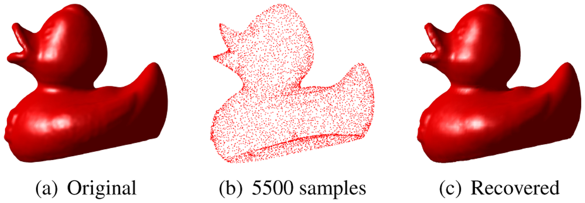
We consider the recovery of a curve from 600 samples using (4) in Fig. 4, where we compare the results with a level-set based scheme introduced in [11]. The regularization parameters of both schemes were adjusted to yield the best results. The results show that the proposed scheme is able to provide good recovery from fewer points. In Fig. 5, we used our proposed algorithm to recover the surface of a duck utilizing randomly chosen samples.

Fig. 4:

Comparison of the proposed curve recovery algorithm with level-set curve recovery [11]. The proposed scheme is capable of yielding good recovery from 600 points.

Fig. 5:

Recovery of 3D surfaces from its random samples. This is an extension of the results in Fig. 4

5.2. Function learning: application to image denoising

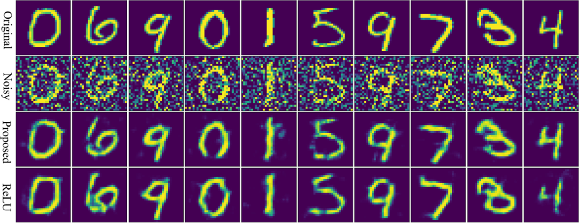
We now apply our function learning framework to the image denoising problem. As discussed previously, the difference between our structure and the commonly used CNN structure is the non-linearity (activation function). We replaced the RELU non-linearity in a network with a single hidden layer and trained the algorithm on the MNIST dataset [12] with added noise. We also trained a RELU network with the same parameters. The testing results are shown in Fig. 6, in which the four columns are corresponding to the original images, the noisy images, the denoising images using RELU and the denoising images using our proposed activation function. From the denoising results, we can see that our proposed activation function provides results that are qualitatively similar to RELU.

Fig. 6:

Comparison of the learned denoiser with Dirichlet activations against RELU networks. The results show that the denoising performance of both methods are comparable.

Note that our activation function has bandwidth as a parameter. In Tab. 1, we compare the denoising performance on 10 testing images in the MNIST dataset with the same noise level. We observe that the performance is not significantly dependent on the assumed bandwidth Γ.

Table 1:

Variation of the PSNR (dB) of the denoised results with the bandwidth of the kernel.

Img.	BW=13	BW=15
1	19.4937	19.5803
2	18.2435	18.4304
3	21.0757	21.2634
4	18.1653	18.8332
5	21.6438	22.7251
6	18.1218	18.4101
7	19.5293	20.3216
8	20.6238	21.1987
9	17.3776	17.9627
10	19.0375	19.4225

6. CONCLUSION

We introduced a data model, where the signals are localized to a surface that is the zero level-set of a bandlimited function ψ. The bandwidth of the function can be chosen as a complexity measure of the surface. We show that the surface can be uniquely recovered using a collection of samples, whose number is equal to the degrees of freedom of the representation. We also use this model to efficiently represent an arbitrary bandlimited function f from points living on the surface. We note that the computational structure of the function evaluation mimics a single layer kernel network.

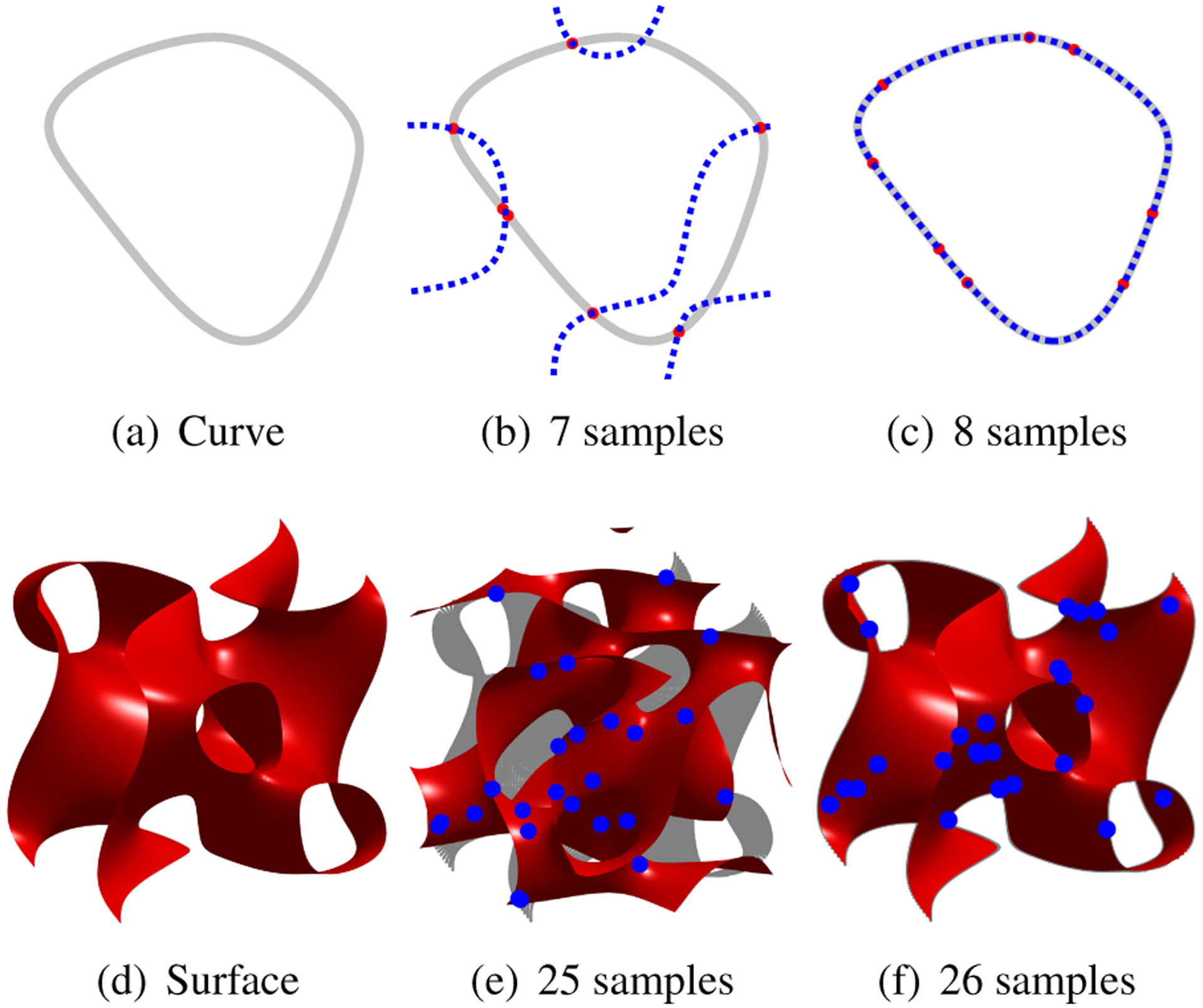
Fig. 1:

Verification of proposition 1 in the 2D and 3D. The 2D curve $\mathcal{C}$ is the zero level set of ψ, whose bandwidth is 3×3. By Proposition 1, we need at least 8 points to recover the curve. Curve recovery failed from a random choice of 7 points (red dots) in (b), while another random set of 8 points succeeded in (c), yielding perfect recovery. For the 3D case, we choose the surface to be the zero level set of a polynomial of bandwidth 3×3×3. Our conclusion requests at least 26 points to recover the surface. (e) and (f) illustrated the conclusion.

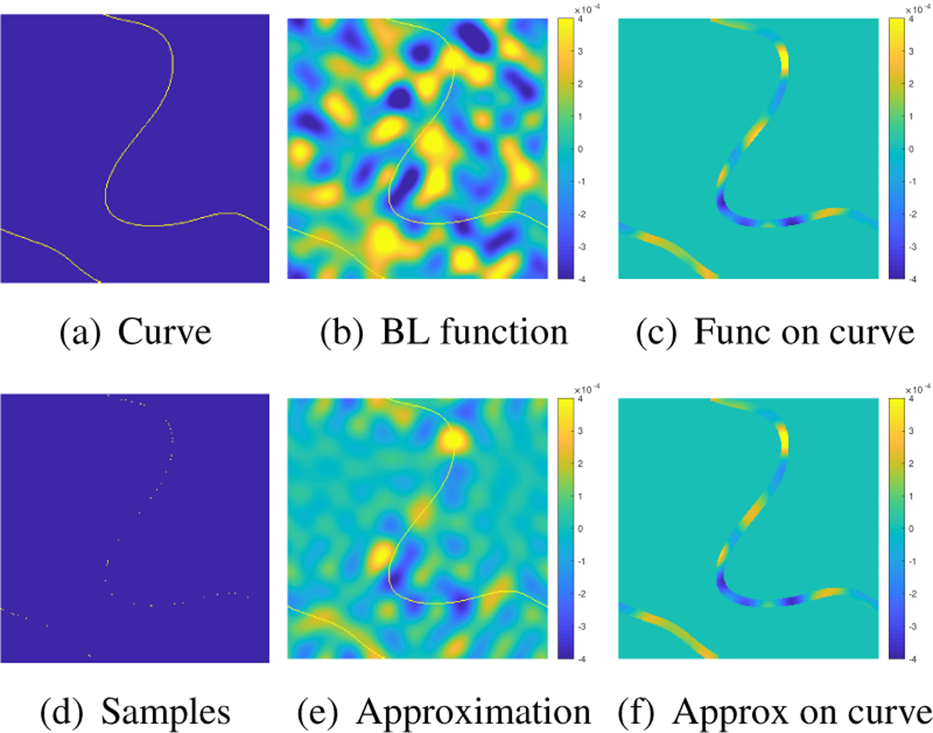
Fig. 2:

Illustration of Proposition 3 on local representation of functions. We consider the local approximation of the bandlimited function in (b) with bandwidth 13×13, on the bandlimited curve shown in (a). The bandwidth of the curve is 3×3. The curve is overlaid on the function in (a) in yellow. The restriction of the function to the vicinity of the curve is shown in (c). Our results in Proposition 3 suggests that the local function approximation requires 13² − 11² = 48 anchor points. We randomly select the points on the curve, as shown in (d). The interpolation of the function values at these points yields the global function shown in (e). The restriction of the function to the curve in (f) shows that the approximation is good.