Generalized Radiographic View Identification with Deep Learning

Abstract

To explore the feasibility of an automatic machine-learning algorithm-based quality control system for the practice of diagnostic radiography, performance of a convolutional neural networks (CNN)-based algorithm for identifying radiographic (X-ray) views at different levels was examined with a retrospective, HIPAA-compliant, and IRB-approved study performed on 15,046 radiographic images acquired between 2013 and 2018 from nine clinical sites affiliated with our institution. Images were labeled according to four classification levels: level 1 (anatomy level, 25 classes), level 2 (laterality level, 41 classes), level 3 (projection level, 108 classes), and level 4 (detailed level, 143 classes). An Inception V3 model pre-trained with ImageNet dataset was trained with transfer learning to classify the image at all levels. Sensitivity and positive predictive value were reported for each class, and overall accuracy was reported for each level. Accuracy was also reported when we allowed for “reasonable errors”. The overall accuracy was 0.96, 0.93, 0.90, and 0.86 at levels 1, 2, 3, and 4, respectively. Overall accuracy increased to 0.99, 0.97, 0.94, and 0.88 when “reasonable errors” were allowed. Machine learning algorithms resulted in reasonable model performance for identifying radiographic views with acceptable accuracy when “reasonable errors” were allowed. Our findings demonstrate the feasibility of building a quality-control program based on machine-learning algorithms to identify radiographic views with acceptable accuracy at lower levels, which could be applied in a clinical setting.

Introduction

Radiography or X-ray imaging is one of the most frequently performed exams in medical imaging. In 2006, about 377 million diagnostic and interventional radiologic examinations were performed in the USA, and over 70% of them were radiographic studies [1]. Although the technology in radiography has developed rapidly over the years, the basic radiographic views, which are images seen by the radiologist, have changed very little. The important factors for describing a radiographic view remain the anatomical region, such as the chest, abdomen, foot; laterality (left or right); projection (antero-posterior, lateral, oblique); and body position, such as supine, erect, flexion, extension. Clinically, when an X-ray order is prescribed, it may contain one or multiple views with clear instructions. For example, an order of “XR Chest 2 View (PA, LAT)” instructs the technologists to take two chest X-ray views for the radiologist’s reading: one posterior-anterior and one lateral.

The predominant equipment in a radiology department for digital imaging is computed radiography (CR) and digital radiography (DR). X-ray images are formatted in digital imaging and communications in medicine (DICOM) and then transferred and stored electronically in the picture archiving and communication system (PACS). The DICOM header contains rich information regarding the patient, exam techniques, and other imaging options. Theoretically, it could also contain information regarding the radiographic views, such as anatomy, laterality, and projections. However, such information is only available for certain vendors, and therefore, it is dependent upon the technologist to select the correct protocol on the workstation prior to the exam. A previous study reported that 15% of exams were missing information about laterality in the header [2]. The current clinical practice requires the X-ray technologists to place additional lead markers indicating laterality and body position, along with the initials of their name. These additional markers could also be added digitally at a later time from the acquisition workstation. The process of adding markers increases the possibility for human error; placement of the wrong markers can lead to wrong-side or wrong-site evaluations and adverse events [3].

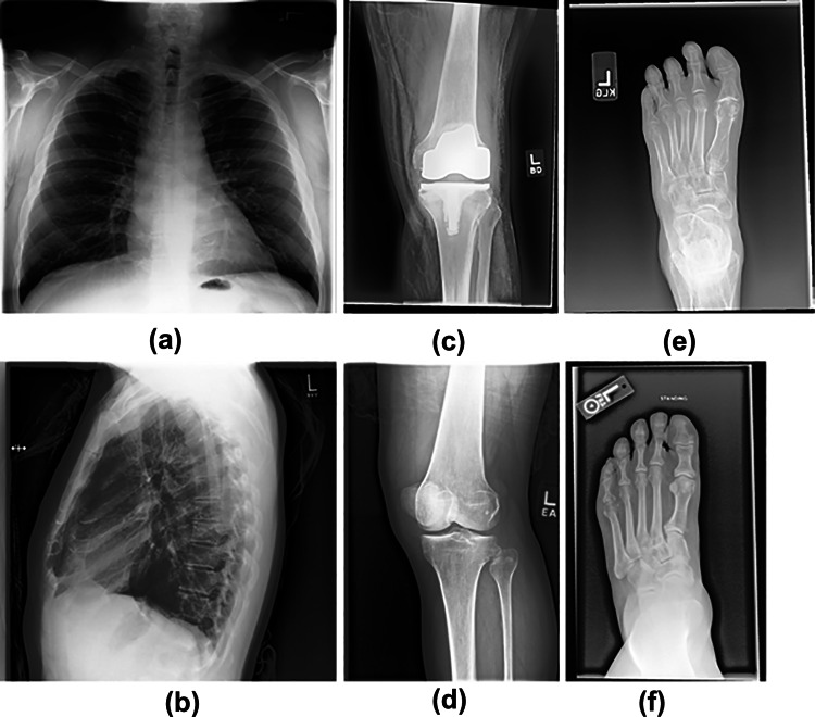
The application of machine learning through the use of the ImageNet Large Scale Visual Recognition Challenge (ILSVRC) has been successfully applied for image classification and object recognition for photographic images [4] as well as applications in the field of radiology using deep learning with pre-trained machine models with transfer learning [5]. Task-specific machine learning models can differentiate types of X-ray views with high accuracy and efficiency, including aspects of laterality [2] and projection [6, 7]. However, the level of difficulty in identifying differences in X-ray views can range from low (chest PA vs. chest lateral, Fig. 1a vs. Fig. 1b), medium (knee AP l vs. oblique, Fig. 1c vs. Fig. 1d), or high (foot normal vs. foot standing, Fig. 1e vs. Fig. 1f).

Fig. 1.

Examples of levels of difficulty in identifying differences in radiographic views: low difficulty: chest PA (a) vs. chest lateral (b); medium difficulty: knee AP (c) vs. oblique (d); high difficulty: foot normal (e) vs. foot standing (f)

This study explored the feasibility of building a general radiography per-image quality control (QC) system based on machine learning. Our QC system was designed to retrieve clinical X-ray images from PACS, identify the exam-type based on the contents of the image, compare the identified exam-type with information from the image header or EMR system, and alert before the images are read by the radiologists and/or the patient walks out of the hospital. As noted above, it can be difficult for machine models to differentiate X-ray views depending on the level of view. Therefore, our QC system was designed to provide output for different levels. The performance of our initial QC system was evaluated retrospectively with current data on PACS and manual labeling. This QC system could be used to identify “big” errors such as wrong site or wrong laterality or “small” mistakes such as wrong angles for oblique exams.

Materials and Methods

IRB approval was obtained for this HIPAA-compliant retrospective study and the requirement of written informed consent was waived. The imaging facility at our institution is contained within a large academic hospital and, in combination with images from affiliated sites, accounts for a total volume of over 150 k radiological exams annually. An initial database search of the electronic medical records (EMR) system (Epic Systems Corporation, Verona, WI, USA) in our facility was performed for all X-ray exams between January 1, 2013 and November 1, 2018, including both CR and DR exams.

Selection of Clinical Images

The exam type was identified based on our internal exam code. Exam types were excluded if they had been performed less than 200 times. For each exam type, we randomly sampled 100 exams after the following exclusion: exams of children (age < 18 years) or multiple exams from the same patient with same exam type. DICOM images of the selected exams were downloaded from our PACS and most contained more than one X-ray view. For instance, a hand exam might include posterior-anterior, lateral, and oblique views.

Image Classes at Four Levels

Each X-ray image was manually assigned to a “class” or “label” at four different levels by an experienced board-certified technologist (LH). The labeling results at the four levels served as the ground truth for training and validation of the proposed machine learning approach for identifying X-ray views. The labeling convention was defined as follows:

Level 1: anatomy level. This level included classes such as “Abd” (abdomen), “Chest”, “Finger”, “Foot”. A total of 25 classes or labels were assigned to this level.

Level 2: laterality level. If a class at the anatomy level had laterality, an additional label was added. If there was no laterality, “None” was assigned. Examples include “Foot_L”, “Finger_R”, “Chest_None”. A total of 41 classes or labels were assigned to this level.

Level 3: projection level. Classes that included projections received an additional label about direction, and if there was no appropriate projection, “None” was added to the assigned label. Examples include “Foot_L_AP”, “Head_None_Lat”, “Abd_None_None”. A total of 108 classes or labels were assigned to this level.

Level 4: detailed level. This was the level with the greatest amount of detailed information for classification. “None” was assigned for images with no additional details. Examples of the detailed level include “Foot_L_AP_Stand”, “Pelvis_None_None_Inlet”, “CSpine_None_AP_Extension”, “Heel_L_AP_None”. In some clinical scenarios, images of the same anatomical area can have subtle differences between views, such as “Foot_R_AP_Reg” vs. “Foot_L_AP_Stand”. In these situations, even experienced technologists require additional information, such as markers in the image, in order to make a correct identification. A total of 143 classes or labels were assigned to this level.

Allowed Labels

Some X-ray views can have an internal ambiguity regarding what label or class is assigned to the image. For example, “wrist” is part of a hand image; however, in some situations, it might be more appropriate to assign the label “wrist” to the image, rather than “hand”. To account for this issue, a series of “allowed labels” was created. “Allowed labels” were assigned for each of the four levels. The following examples demonstrate “Allowed labels” for each level of “Hand”: level 1 (hand) = ‘Finger’, ‘Wrist’; level 2 (Hand_L) = ‘Finger_L’, ‘Wrist_L’; level 3 (Hand_L_Lat) = ‘Finger_L_Lat’, ‘Wrist_L_Lat’; and level 4 (Hand_L_Lat_None) = ‘Finger_L_Lat_None’, ‘Wrist_L_Lat_None’. We also calculated performation evaluation with “allowed labels” as “Allowed_Sensitivity.

Deep Learning Model and Transfer Learning

Machine learning models were trained with a Linux-based computer using the Keras deep learning library (Version 2.2.2) [8] with TensorFlow backend (Version 1.10.0) and CUDA 9.1 (Nvdia Corporation, Santa Clara, CA) for GPU acceleration.

To prepare the image datasets for model training and testing, all original images in DICOM format were converted to PNG format (Python Library matplotlib version 3.0.0). These images were then resized to 299 × 299 pixels, and pixel values were normalized to [0, 1] with the standard Keras image preprocessing process (keras.preprocessing.image). The constructed datasets were randomly split into training sets (70%), validation sets (15%), and test sets (15%), which were used to train four models to make predictions for each of the four levels (anatomy, laterality, projection, detailed). Real-time data augmentation was performed by applying the following random image transformations: image rotation (− 10° to 10°), image translation (60 pixels each direction), image shearing (− 10° to 10°), and image zooming (0–20%) for each epoch. In addition, horizontal flip was turned on only for level 1 classification data augmentation, because the image orientation could be an important feature in classifying the laterality.

Inception V3 [9] was selected to perform the classification task in this study. Inception V3 was pre-trained with the ImageNet database [4]. This infrastructure has demonstrated a promising capacity for image classification in several settings [10, 11]. Transfer learning adjusted the model parameters to fit the radiography data. Initial weights of the model were set as “imagenet” [9], which is the default in Keras. The top layer of the original Inception V3 was removed and the following four layers were added: (1) a pooling layer, with GlobalMaxPooling2D matching the size of original Inception V3 model output; (2) a fully connected DENSE layer with activation function “relu”; a dropout layer (dropout rate 0.5); and a final activation layer with sigmoid activation and an output size equal to the number of classes. Categorical cross-entropy was used as the loss function and learning rate was set to be 0.0001, with the total number of epochs set at 40. For each level of the classification task, the same neural network infrastructure was trained and validated, yielding four separate models for four levels of labeling.

Model Output

The output of the model on each image is a vector of “scores” corresponding to each class. The “predicted class” was defined as the output class with the highest score. We repeated the processing for all four levels, respectively.

To understand the essential features recognized by the neural network for making classification decision, we generated a “heat map” for each prediction task, based on a gradient-weighted class activation mapping (Grad-CAM) approach [12].

Performance Evaluation

Performance of classification models evaluated with ImageNet Large Scale Visual Recognition Challenge (ISLVRC) classification task [4] uses a top 5 classification error. This top-n performance metric indicates the tolerance level of the prediction errors for multi-label situations. We did not adopt this concept for this study because the error could be either “reasonable” (hand vs. wrist) or “unreasonable” (left vs. right or knee vs. elbow). Instead, we introduced the concept of “Allowed Label” to evaluate tolerance only for “reasonable” errors.

Each class was evaluated for sensitivity (true positive rate, or 1-false negative rate), positive predictive value (PPV), and precision (accuracy). It should be noted that in this model, the class distribution impacts the PPV, which differs from real-life situations. Model performance was also evaluated for “Allowed Label” when “reasonable” errors in the pre-defined list of classes were forgiven.

The following metrics evaluated performance for each class:

Sensitivity = TP/(TP + FN)

PPV = TP/(TP + FP)

The overall performance for each level was evaluated with the following metric:

Accuracy = (TP + TN)/(TP + TN + FP + FN)

where TP = true positive; FP = false positive; TN = true negative; and FN = false negative.

In addition, performance of “AllowedLabel_Sensitivity” was evaluated for each class. If the prediction was one of the “Allowed Labels” for that class, then the prediction was assumed correct.

To examine uncertainty of results for performance metrics of sensitivity and PPV, the bootstrap method (n = 1000) was used to determine the mean and 95% confidence interval (CI).

Results

After applying the selection criteria, 120 X-ray exam types were identified and included for the construction of the database. The final constructed database included a total of 15,046 images, which comprised 143 X-ray views (level 4 classes), from 23 different radiographic unit models, and 7 different vendors in 9 clinical sites affiliated with our institution. These images were manually assigned to 25 classes at the anatomy level (level 1), and these were subsequently assigned to laterality, projection, and detailed levels (levels 2, 3, and 4, respectively).

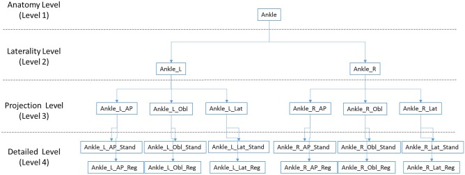
Table 1 shows the Allowedlabel_Sensitivity of the classes at level 1 and the corresponding performance distribution [minimum, maximum] for classes at levels 2, 3, and 4. For each increase in level, if there was a new assigned label, there was an increase in classes. The class for “Ankle” at level 1 increased to Ankle_L and Ankle_R at level 2. This increase continued to level 4, resulting in a four-level tree hierarchy for “Ankle”, as illustrated in Fig. 2. However, if “None” was assigned at the next level, there was no increase in number of classes. As shown in Table 1, there was no increase in classes for “Abd” until level 4.

Table 1.

Performance (Allowed_Sensitivity) of the 25 assigned classes at level 1, and the number of assigned classes (n) and performance distribution [Min, Max] at levels 2, 3, and 4

	Level 1 (anatomy)	Level 2 (laterality)		Level 3 (projection)		Level 4 (detail)
Class	Performance	(n)	Performance	(n)	Performance	(n)	Performance
Abd	0.99	1	[0.98, 0.98]	1	[0.98, 0.98]	2	[0.86, 1.00]
Chest	1.00	1	[1.00, 1.00]	2	[0.96, 1.00]	3	[0.74, 1.00]
Ribs	0.98	2	[0.77, 0.80]	2	[0.88, 0.91]	6	[0.38, 0.83]
Ankle	1.00	2	[0.95, 1.00]	6	[0.93, 1.00]	12	[0.64, 1.00]
Femur	0.95	2	[0.99, 0.99]	12	[0.78, 1.00]	12	[0.67, 1.00]
Foot	1.00	2	[0.97, 1.00]	6	[0.90, 1.00]	10	[0.84, 1.00]
Heel	0.98	2	[0.93, 0.97]	4	[0.90, 1.00]	4	[0.82, 1.00]
Hip	1.00	2	[1.00, 1.00]	6	[1.00, 1.00]	6	[0.82, 1.00]
Pelvis	0.96	1	[1.00, 1.00]	1	[1.00, 1.00]	3	[0.79, 1.00]
Knee	1.00	2	[0.92, 0.92]	8	[0.67, 1.00]	8	[0.80, 1.00]
TibFib	0.96	2	[0.85, 0.91]	4	[0.82, 0.95]	4	[0.75, 0.89]
Toe	0.97	2	[0.84, 0.97]	4	[0.81, 1.00]	4	[0.81, 1.00]
Shoulder	0.99	2	[0.96, 0.97]	8	[0.82, 1.00]	12	[0.00, 1.00]
Elbow	1.00	2	[0.93, 0.96]	6	[0.77, 1.00]	6	[0.68, 1.00]
Finger	1.00	2	[0.80, 1.00]	4	[0.50, 0.92]	4	[0.67, 1.00]
Forearm	1.00	2	[1.00, 1.00]	4	[0.91, 1.00]	4	[0.82, 1.00]
Hand	1.00	2	[0.99, 1.00]	8	[0.84, 1.00]	8	[0.70, 1.00]
Humerus	0.96	2	[0.97, 0.98]	4	[0.84, 0.94]	4	[0.88, 1.00]
Wrist	1.00	2	[0.97, 0.99]	4	[0.86, 1.00]	8	[0.61, 1.00]
Head	1.00	1	[1.00, 1.00]	4	[0.67, 1.00]	4	[0.94, 1.00]
Neck	1.00	1	[1.00, 1.00]	2	[1.00, 1.00]	2	[1.00, 1.00]
CSpine	1.00	1	[1.00, 1.00]	2	[1.00, 1.00]	6	[0.59, 1.00]
TSpine	0.98	1	[0.98, 0.98]	2	[0.91, 1.00]	3	[0.94, 1.00]
LSpine	1.00	1	[0.99, 0.99]	2	[0.98, 1.00]	5	[0.35, 1.00]
Sacrum	1.00	1	[1.00, 1.00]	2	[0.91, 0.96]	3	[0.85, 1.00]
All		41		108		143

Fig. 2.

Example of a hierarchical classification tree for labeling radiographic images of the “Ankle” showing the increase in number of classes with each level. Level 1: anatomy level; level 2: laterality level (n = 2); level 3: projection level (n = 6); and level 4: detailed level

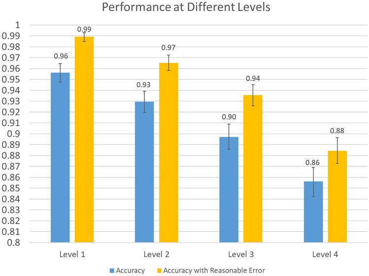
The mean and 95% confidence intervals for sensitivity, PPV for each class of exam type, including Allowedlabel_Sensitivity for “Allowed Labels” at levels 1, 2, 3, and 4 are shown in supplementary Tables S1–S4. As the classification level increased, there was a decrease in the overall performance (mean ± SD) for sensitivity, PPV, and Allowed_Sensitivity from 0.95 ± 0.05, 0.95 ± 0.04, and 0.99 ± 0.02, respectively, at level 1 to 0.86 ± 0.16, 0.85 ± 0.16, and 0.89 ± 0.16, respectively, at level 4. We also investigated the impact of allowing for “reasonable errors” by comparing accuracy with and without “allowed labels”. As shown in Fig. 3, without “Allowed labels” the overall accuracy was 0.96, 0.93, 0.90, and 0.86 for levels 1, 2, 3, and 4, respectively. However, application of “Allowed Labels” increased overall accuracy to 0.99, 0.97, 0.94, and 0.88 for levels 1, 2, 3, and 4, respectively.

Fig. 3.

Bar graph demonstrates differences in performance at levels 1, 2, 3, and 4. Blue bar indicates overall accuracy. Orange bar shows accuracy improves at all four levels when “Allowed labels” are included to account for “reasonable errors”. Error bars = 95% confidence interval

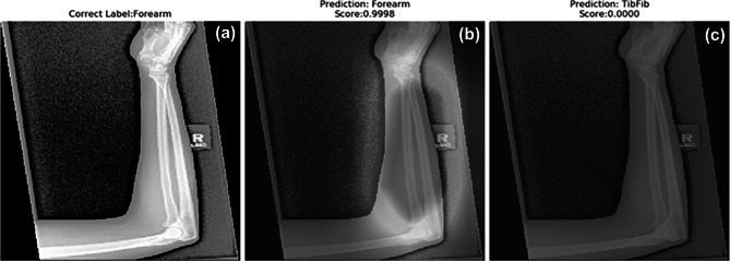
Representative images demonstrating the correct prediction of a level 1 case are shown in Fig. 4. The original image (Fig. 4a), labeled as “Forearm”, was predicted correctly, as demonstrated by the high score of 0.9998 (Fig. 4b). The QC system did not identify the image as “TibFib”, which is confirmed by the prediction score of 0.000 (Fig. 4c). The successful level 1 classification is further corroborated by the overlap of the peak intensity regions in the heat map shown in Fig. 4b with the original X-ray image in Fig. 4a.

Fig. 4.

Representative images from a level 1 case with a correct prediction: (a) the original image was labeled “Forearm”; (b and c) heatmap images indicating area for model prediction; (b) the correct prediction of “Forearm” and the prediction score = 0.9998 indicates a high level of confidence in the model classification; (c) the prediction score = 0.0000 for the image classification indicates a low level of confidence that the prediction of “TibFib” is correct

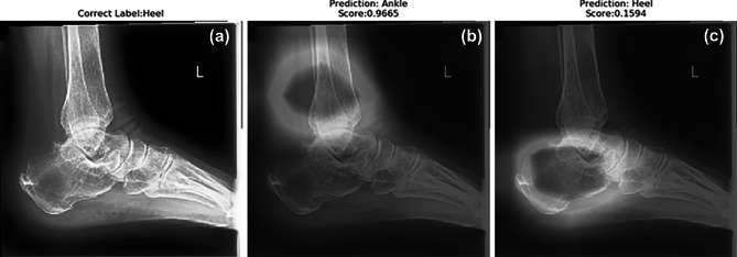
The representative images in Fig. 5 demonstrate an instance of an incorrect prediction for a level 1 case. The original image (Fig. 5a) labeled as “Heel” was predicted as “Ankle” and received a high score of 0.9665 (Fig. 5b). When the image was correctly identified as “Heel”, the prediction score was only 0.1594 (Fig. 5c). This figure also provides evidence for the importance of accommodating ambiguity in an X-ray image as well as multi-labels and the effect on classification accuracy. The identification of the original image as “Ankle” could be considered a “reasonable error” because it is part of the image. By applying “Allowed Labels” for “Heel” at level 1, which includes “Ankle”, the “AllowedLabel_Sensitivity” includes the prediction for “Ankle”.

Fig. 5.

Representative images from a level 1 case with an incorrect prediction: (a) the original image was labeled “Heel”; (b) the prediction score = 0.9665 indicates a high level of confidence in the incorrect classification of the label “Ankle” for the image; (c) although this image was labeled correctly as “Heel”, the prediction score = 0.1594 indicates a low level of confidence in the prediction. The prediction in (b) is an example of the advantage of “Allowed Labels” for improving performance. “Ankle” is an “Allowed Label”, for “Heel”, which improves performance when calculating “AllowedLabel_Sensitivity”

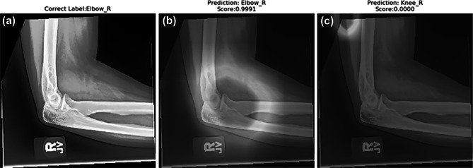
Classes at level 2 require the system to predict not only the class, but also laterality. Representative images of predictions for a level 2 case are shown in Fig. 6. The original X-ray image was labeled as “Elbow_R” (Fig. 6a). The image was correctly predicted as “Elbow_R” and received a high score of 0.9991 (Fig. 6b). The prediction for Fig. 6c was “Knee_R”, and the prediction score of 0.0000 indicates no confidence that the prediction was correct. The peak intensity region of the generated heat map shown in Fig. 6b is located in the lateral region of the anatomy, suggesting that the correct prediction (Elbow_R) was based on the anatomical features, rather than of the marker placed by the technologist.

Fig. 6.

Representative images from a level 2 case with a correct prediction: (a) the original image was labeled “Elbow_R”; (b) the image was classified as “Elbow_R”, correct for the anatomy as well as the laterality of level 2 and the prediction score = 0.9991 indicates a high level of confidence in the prediction; (c) the heatmap in the image is above the elbow and was classified as “Knee_R, and the prediction score of 0.0000 indicates no confidence in the prediction

Discussion

This study investigated the performance of a state-of-the-art machine-learning model designed for the task of classification of X-ray images. Performance results demonstrated the feasibility of building an automatic QC system for the practice of diagnostic radiography. The model performance was evaluated at different levels of difficulty, from the simple anatomy level (level 1) to the more challenging detailed level (level 4), which requires identifying subtle differences in images. We found the overall accuracy of classification matched the difficulty of different levels; values ranged from 0.96 at level 1 to 0.86 at level 4. When “Allowed Labels” were added to allow for “reasonable errors”, values increased to 0.99 at level 1 and 0.90 at level 4.

It is desired to have an automatic quality control program in diagnostic radiography. In current clinical practice, technologists manually perform image quality control/assessment before the exams are sent to the PACS system. Common medical errors such as incorrect patient position, exam type, or laterality occur because the manual process is prone to errors due to variable viewing conditions and the dependence on the personal experience of the technician. Although the occurrence an X-ray performed incorrectly without post-identification of errors is small, the consequences can be severe, including a misdiagnosis or an inaccurate evaluation of treatment [3]. The application of machine learning techniques could mitigate these medical errors by providing an automatic quality control system. Our results demonstrate that the emerging machine learning approach can be used to identify X-ray images at different levels with reasonable accuracy.

Deep learning has been demonstrated to be capable of performing image classification tasks [4, 13, 14] at a level of performance comparable with humans. The available dataset from ISLVRC [4] uses images for classification, with an error rate of approximately 6%. Without other benchmarks, a similar performance for classification models in radiography view identification would be expected. The error rates (1-accuracy) in our study fall into this range, for level 1 (4%) and level 2 (7%); however, levels 3 and 4 had error rates of 10% and 12%, respectively. We were able reduce alert numbers by introducing “allowed label” to tolerate “reasonable” errors in our QC system based on this algorithm, and the resulting error rate dropped to 1%, 3%, 6%, and 10% for levels 1, 2, 3, and 4, respectively. Assuming a radiology facility has a daily volume of 200 patients, a 3% error rate would lead to an acceptable number of less than 10 false alarms. An error rate greater than 3% might lead to alert fatigue and reduce the effectiveness of the QC system. Therefore, our findings suggest that the initial build of the automatic QC system should work at the anatomy and laterality levels, but not at the projection and detailed level.

The introduction of an “allowed label” setting in this study added tolerance for “reasonable errors”. This addition reduced the alarm rate for the QC system, especially when exam types included a similar anatomical region and/or orientation. “Allowed label” also served as a user-adjustable option for different clinical scenarios. For example, in a multi-purpose radiographic room, “Abdomen” is currently an allowed label for “Chest” images; however, in a chest-only room, the QC system can be adjusted to exclude “Abdomen”. In addition, our results indicated that applications in which “allowed labels” should be excluded, such as providing suggestions to fill in DICOM body part tags, this method performed with 96% accuracy for level 1 view identification.

The model performance could be further improved with several approaches. Currently, our model prediction is based on the contents of the image. Combining with or cross-checking the reference information from EMR orders and DICOM headers could improve the performance. We did not train our model to focus on the markers. Although the literature shows if a separate model is used to focus on the marker information, accuracy for detection of laterality can be improved up to 99% [2], assuming the marker information is correct. More specific tasks will improve the model performance as well. For example, 100% accuracy can be obtained if the machine learning algorithms are only trained to differentiate two views (chest PA or lateral) [7], or AUC = 1 in differentiate CC vs MLO view (Mammo views) [6]. The improvement of model structures is occurring daily and inclusion of more data will possibly improve performance further, leading to a more feasible automatic QC system.

There were some data variations inside each class which affected the model performance. Some variations were the result of natural anatomic differences in the body, such as height, weight, sex, and age. Some variations were due to the physiological changes that accompanied the clinical symptoms, such as broken bones in any area of the body, pulmonary edema in the chest, or implants in the pelvis. The definition of the view itself also caused variations in data. For example, “Finger_L_Obl_None” contained images for all five fingers. Future studies could benefit from a larger dataset, which should improve the generality of the model performance, and increase the detection of subtle differences between similar classes.

Further studies could address the problem of hierarchy in the classification task with a different approach. We trained one general model for each level to identify all views, which may have had the disadvantage of introducing additional errors at each level. For example, at level 3, the view for an image labeled “Elbow_Left_AP” might be wrongly identified as “Elbow_Right_AP”, and the error actually occurred at level 2. An alternate approach would be a “cascade” classification, which would train different models at different levels for specific tasks. This could be achieved by first obtaining the level 1 classification, such as “Knee”, and then training a second model whose purpose is to differentiate “Knee_Left” or “Knee_Right” at level 2. With each classification task, the number of classes should be significantly reduced, and thus, the performance should improve. However, this “Cascade” classification will require a significantly larger number of models, and in this situation, the task has to be specified individually.

The next step of this project will be to include more data in the datasets, with an emphasis on including other institutions in the data source, if possible. We also expect to have a platform that could provide near real-time feedback to the technologists (a few minutes after PACS upload), to reduce the possible wrong side, wrong exam errors in radiology.

Conclusions

Machine learning methods were developed, and individually applied on a comprehensive X-ray image dataset consisting of 15,046 different images. The X-ray images were classified at four levels: level 1 (anatomy level), level 2 (laterality level), level 3 (projection level), and level 4 (detailed level). Model performance was reported for both strict definition and allowing for “reasonable errors”. Acceptable performance was observed when “reasonable errors” were allowed, indicating the possibility of building a machine-learning-based X-ray quality control system.

Electronic supplementary material

Below is the link to the electronic supplementary material.

Supplementary information

The online version of this article (10.1007/s10278-020-00408-z) contains supplementary material, which is available to authorized users.

References

- 1.Mettler FA, Jr, et al. Radiologic and nuclear medicine studies in the United States and worldwide: frequency, radiation dose, and comparison with other radiation sources–1950-2007. Radiology. 2009;253(2):520–31. doi: 10.1148/radiol.2532082010. [DOI] [PubMed] [Google Scholar]
- 2.Filice RW, Frantz SK. Effectiveness of Deep Learning Algorithms to Determine Laterality in Radiographs. J Digit Imaging. 2019;32(4):656–664. doi: 10.1007/s10278-019-00226-y. [DOI] [PMC free article] [PubMed] [Google Scholar]
- 3.Seiden SC, Barach P. Wrong-side/wrong-site, wrong-procedure, and wrong-patient adverse events: Are they preventable? Arch Surg. 2006;141(9):931–9. doi: 10.1001/archsurg.141.9.931. [DOI] [PubMed] [Google Scholar]
- 4.Russakovsky O, et al. ImageNet Large Scale Visual Recognition Challenge. International Journal of Computer Vision. 2015;115(3):211–252. doi: 10.1007/s11263-015-0816-y. [DOI] [Google Scholar]
- 5.Litjens G, et al. A survey on deep learning in medical image analysis. Med Image Anal. 2017;42:60–88. doi: 10.1016/j.media.2017.07.005. [DOI] [PubMed] [Google Scholar]
- 6.Yi PH, et al. Deep-Learning-Based Semantic Labeling for 2D Mammography and Comparison of Complexity for Machine Learning Tasks. J Digit Imaging. 2019;32(4):565–570. doi: 10.1007/s10278-019-00244-w. [DOI] [PMC free article] [PubMed] [Google Scholar]
- 7.Rajkomar A, et al. High-Throughput Classification of Radiographs Using Deep Convolutional Neural Networks. J Digit Imaging. 2017;30(1):95–101. doi: 10.1007/s10278-016-9914-9. [DOI] [PMC free article] [PubMed] [Google Scholar]
- 8.Chollet FCO and others, Keras. 2015, https://github.com/fchollet/keras
- 9.Szegedy C, et al: Rethinking the inception architecture for computer vision. in Proceedings of the IEEE conference on computer vision and pattern recognition(CVPR), 2016, pp 2818-2826
- 10.Hussain M, Bird JJ, Faria DR, et al. A Study on CNN Transfer Learning for Image Classification. Advances in Computational Intelligence Systems (Ukci) 2019;840:191–202. doi: 10.1007/978-3-319-97982-3_16. [DOI] [Google Scholar]
- 11.Ramcharan A, et al: Deep Learning for Image-Based Cassava Disease Detection. Frontiers in Plant Science, 2017, 8, pp 1852 [DOI] [PMC free article] [PubMed]
- 12.Selvaraju RR, et al. Grad-CAM: Visual Explanations from Deep Networks via Gradient-based Localization. Ieee International Conference on Computer Vision (Iccv) 2017;2017:618–626. doi: 10.1109/ICCV.2017.74. [DOI] [Google Scholar]
- 13.Esteva A, et al. Dermatologist-level classification of skin cancer with deep neural networks (vol 542, pg 115, 2017) Nature. 2017;546(7660):686–686. doi: 10.1038/nature22985. [DOI] [PubMed] [Google Scholar]
- 14.Majkowska A, et al: Chest Radiograph Interpretation with Deep Learning Models: Assessment with Radiologist-adjudicated Reference Standards and Population-adjusted Evaluation. Radiology, 2020 Feb; 294(2) pp 421-431 [DOI] [PubMed]
Associated Data
This section collects any data citations, data availability statements, or supplementary materials included in this article.