Using LSTMs to Learn Physiological Models of Blood Glucose Behavior

Abstract

For people with type 1 diabetes, good blood glucose control is essential to keeping serious disease complications at bay. This entails carefully monitoring blood glucose levels and taking corrective steps whenever they are too high or too low. If blood glucose levels could be accurately predicted, patients could take proactive steps to prevent blood glucose excursions from occurring. However, accurate predictions require complex physiological models of blood glucose behavior. Factors such as insulin boluses, carbohydrate intake, and exercise influence blood glucose in ways that are difficult to capture through manually engineered equations. In this paper, we describe a recursive neural network (RNN) approach that uses long short-term memory (LSTM) units to learn a physiological model of blood glucose. When trained on raw data from real patients, the LSTM networks (LSTMs) obtain results that are competitive with a previous state-of-the-art model based on manually engineered physiological equations. The RNN approach can incorporate arbitrary physiological parameters without the need for sophisticated manual engineering, thus holding the promise of further improvements in prediction accuracy.

I. Introduction and Motivation

People with type 1 diabetes (T1D) are faced with the daunting task of continually monitoring their blood glucose levels (BGLs) and correcting them whenever they are too high (hyperglycemia) or too low (hypoglycemia). Achieving and maintaining good blood glucose (BG) control is key to avoiding serious disease complications [1]. If BGLs could be accurately predicted 30 to 60 minutes in advance, patients could proactively prevent hyper- and hypoglycemia, improving BG control and enhancing health and well-being.

The Artificial Pancreas project [2] has sparked interest in BG prediction. This project aims to provide a closed-loop control algorithm that inputs BGLs from a continuous glucose monitoring (CGM) system and instructs an insulin pump to deliver the right amount of insulin to keep BGLs in range [3], [4]. There have been several research efforts to predict BGLs of late [5]–[8]. However, the use of small or simulated patient datasets has limited progress.

We have assembled a database containing over 1,600 days of actual patient data through our work on intelligent decision support for patients with T1D on insulin pump therapy [9]–[14]. This data includes not only continuous BGLs from sensors, but also factors known to influence BGLs, including insulin, food, exercise, and sleep. As previously reported [10], [11], we have already used this data with physiologic models of BG dynamics to train patient-specific time series prediction models within a support vector regression (SVR) framework. Evaluation showed that the trained BGL prediction models outperformed our three diabetes experts [11].

An important part of our research is focused on the identification of additional types of signals that could further increase the performance and reliability of the BG level prediction models. In particular, new portable sensing technologies have been developed recently for providing almost continuous measurements of an array of physiological parameters that include heart rate, skin conductance, skin temperature, and properties of body movements such as acceleration. However, the impact that the sensor measurements have on BG prediction performance will depend on the proper modeling of their relations with the other variables in the system. One approach would be to reengineer the current physiological model, which captures only carbohydrates, insulin, and glucose, to also incorporate the new physiological parameters. Reengineering the physiological model would require formulating other possibly nonlinear state transition equations such that their predictions match observed blood glucose behavior. This could be very time consuming and cognitively demanding, while lacking in scalability: as new types of physiological parameters become available, the physiological model would have to be reengineered again. Instead, we propose to leverage recent advances in unsupervised feature learning and deep learning (UFLDL) in order to build a platform that can seamlessly incorporate any number of physiological variables. The core idea behind many successful UFLDL methods is that complex highly-varying functions (e.g. blood glucose) can be learned using simple algorithms, by training on mostly unlabeled data [15]. While a trained UFLDL model is very complex, the learning algorithm itself is usually very simple: the complexity of the trained model comes from the data, not from the algorithm [16]. Over the years, a number of approaches to BG prediction have used RNNs, as reviewed in [17]. Previous approaches use plain RNNs, which are difficult to train due to vanishing gradients, a problem that is often compounded by the limited size of the clinical data used in experimental evaluations. In contrast, we propose an RNN architecture that uses LSTM units, which are not affected by the vanishing gradient problem. The LSTM architecture is trained and evaluated on a dataset of 5 patients, containing approximately 400 days worth of BG levels, insulin, and meal event data.

II. Engineered Physiological Model

A physiological model of blood glucose behavior is a continuous dynamic model in which a state transition function computes the next state of the system given the current state and input variables. The overall blood glucose dynamics is usually characterized into three compartments: meal absorption dynamics, insulin dynamics, and glucose dynamics [18]–[20]. For our physiological model from [11], which is summarized here, we adapted the state transition equations from [21] to better match published data and feedback from a diabetes expert. The equations for the state transition function use a set of parameters α and are shown below for each of the three compartments.

1. Meal absorption dynamics (U_C represents meal carbs):

   • C_g1 (t + 1) = C_g1 (t) − α_1C * C_g1 (t) + U_C (t) [consumption]
   • C_g2 (t + 1) = C_g2 (t) − α_1C * C_g1 (t) – α_2C / (1 + 25/C_g2 [digestion]
2. Insulin dynamics (U_I represents injected insulin):

   • I_S (t + 1) = I_S (t) – α_fi * I_S (t) + U_I(t) [injection]
   • I_m (t + 1) = I_m (t) – α_fi * I_S (t) – α_ci * I_m (t) [absorption]
3. The general equation for the glucose compartment is G_m (t +1) = G_m (t) + Δ_abc – Δ_ind – Δ_dep – Δ_clr + Δ_egp, where:

   • Δ_abc = α_3C * α_2C/(1 + 25/C_g2 (t)) [absorption]
   • ${\Delta }_{ind}={\alpha }_{1ind}*\sqrt{G(t)}$ [insulin independent utilization]
   • Δ_dep = α_1dep * I (t) * (G (t) + α_2dep)[insulin dependent utilization]
   • Δ_clr = α_1clr * (G (t) − 115) [renal clearance, only when G(t) > 115)]
   • Δ_egp = α_2egp * exp(−I (t)/α_3egp) –α_1egp * G (t) [endogenous liver production]

The glucose and insulin concentrations are computed deter-ministically from their mass versions as follows, where bm stands for the body mass and IS is the insulin sensitivity:

• G(t) = G_m (t)/(2.2 * bm)

• I(t) = I_m (t) * IS/(142 * bm)

Figure 1 shows the dependencies that the state transition functions above induce among the state variables of the engineered physiological model (EPM).

Fig. 1.

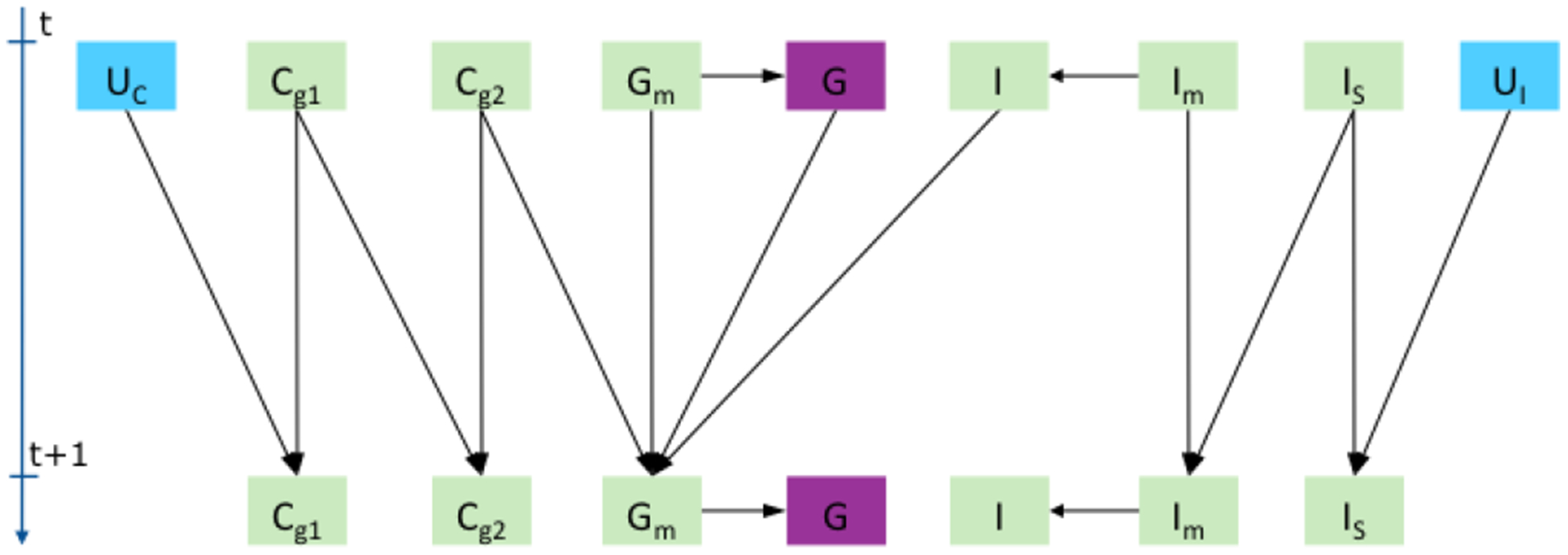
Physiological dependencies between input U (blue), state (green), and output (violet) variables for carbs (C), insulin (I), and glucose (G).

The state transition equations were used in an extended Kalman filter (EKF) [22], which models the noise inherent in the BGL sensor and meal data. The EKF model ran a state prediction step every minute and a correction step every 5 minutes, corresponding to the sampling interval used by the CGM system. The physiological model parameters α and the state transition equations were adapted to match published BGL behavior and feedback from our doctors, who were shown graphs of the time-dependent behavior of the state variables in the model. The EKF model was first used on its own to make BG level predictions, by running it in prediction mode only during the 30 or 60 minutes of the prediction region, however results were not better than the simple t₀ baseline that predicts the BG level stays the same. This was not surprising, given that patients with diabetes can vary significantly in how they respond to insulin or carbohydrate intake. Therefore, a personalized model was built for each patient by training a Support Vector Regression (SVR) model [23] on a feature representation that was derived from the state vector computed by the EKF on top of the physiological model. This approach is described in detail in [11], where it was shown to outperform the predictions of the three diabetes experts participating in the study. In this section, we report the results of the SVR prediction model using a simpler tuning procedure and two different training scenarios.

A. Evaluation Dataset

We used the original evaluation dataset from [11], containing 200 timestamps collected from 5 T1D patients, 40 points from each. The timestamps were sampled manually to capture a diversity of situations: different times during the day or night; close to or far from daily events; on the rising, decreasing, or flat sections of the BG curves; around or far from past or future local minima or maxima of the BGL; or in the vicinity of inflection points. We call these 5 patients the test patients or the test dataset. Furthermore, 5 other patients from the same clinical study were selected to provide data for tuning the model hyper-parameters. We call these additional 5 patients the development patients or the development dataset. For each patient, the data provided to the system consists of blood glucose levels measured every 5 minutes by a CGM system, information about boluses (time, type, and amount of insulin), the basal rate, and meals (time and carbohydrate amount).

B. Experimental Evaluation

Some of the timestamps in the test dataset had insulin or meal events in the prediction region, i.e. between the prediction time t₀ and the prediction horizon t₀ + 30 or t₀ +60 minutes in the future - there were 30 such points for the 30 minute horizon and 65 for the 60 minute horizon. Consequently, we re-evaluated the EPM-based prediction model, which was introduced in [11] and summarized above, in the following two scenarios:

1. What-if: In this scenario, insulin or meal events that happened during the prediction region were still used as inputs for the physiological model in that region. This is how both the physiological model and the diabetes experts were evaluated in [11]. For prediction points that had such events, this could be seen as evaluating the model in a what-if scenario, e.g. what would the BG level be 60 minutes from now if the patient had a snack containing 100 grams of carbs 20 minutes from now.

2. Agnostic: In this scenario, any insulin or meal events that happened during the prediction region were ignored by the physiological model.

For each point in the dataset, the SVR model was trained on the previous week of data. The hyper-parameters of the SVR were tuned separately for each point in [11], by using one week of data before the training week. This tuning procedure is computationally expensive and unfeasible in a real-time setting. Therefore, we used instead the same generic set of hyper-parameters for all points in the dataset, by tuning the SVR on a patient from the development dataset. Using a generic set of hyper-parameters also makes the SVR evaluation consistent with the LSTM evaluation from the next section, for which we used a similar tuning approach.

Table I shows the RMSE of the EPM-based SVR model in the two evaluation settings, compared with a t₀ baseline that predicts the BG level stays the same, and an Auto Regressive Integrated Moving Average (ARIMA) model trained on BG levels using model identification as detailed in [11].

TABLE I.

RMSE results for the EPM-based SVR model in Agnostic and What-if settings vs. t₀ and ARIMA baselines.

Horizon	t0	ARIMA	Agnostic	What-if
30 min	27.5	22.9	21.6	20.3
60 min	43.8	42.2	39.2	35.5

III. Trained Physiological Model

Figure 2 shows a recurrent neural network architecture with one hidden layer that captures the same dependencies as the EPM from Figure 1: the hidden state variables H at time t + 1 depend recursively on the hidden state variables at time t, as well as on the input variables U at time t + 1 and the glucose value G at time t. As opposed to the EPM approach where the dependencies are modeled through manually engineered state transition equations, the RNN approach models the same dependencies through the weights of the connections between the input layer and the hidden layer. Nonlinear behavior of the hidden state variables is captured through the use of nonlinear activation functions at the output of the hidden layer neurons. As a consequence of the universal approximation theorem [24], with a sufficient number of hidden neurons, the RNN architecture in Figure 2 is general enough to approximate the physiological model from Section II, no matter what state transition equations are used. A significant advantage of the RNN architecture is that it can accommodate any new types of physiological parameters, as sensor measurements for those parameters become feasible to acquire. This would be done simply by increasing the size of the input vector U_t+1 to contain the new sensor measurements for the time interval [t, t + 1).

Fig. 2.

An RNN architecture capturing similar dependencies between hidden state variables (green), input variables (blue), and the output glucose variable (violet). Thick arrows between layers represent full connections. The inputs can be optionally connected to the output layer.

The RNN architecture could be trained first to predict the BG level at the next time step, i.e. only the first element G_t+1 of the output layer shown in Figure 2. In the second step, the RNN would be trained to use the physiological dependencies captured by the hidden layer neurons to make predictions at predefined time intervals, such as 30 and 60 minutes into the future. Correspondingly, the output layer would contain two additional nodes, one for 30 and another for 60 minute prediction. In the experiments reported in this paper, we adopted a simpler approach in which the RNN is trained in separate experiments to directly make either 30 or 60 minute predictions.

While RNNs are a powerful tool for time series modeling, training them is not easy, mainly due to the vanishing gradient problem [25], [26], which makes it difficult to learn long-term dependencies. To alleviate this, we use long short-term memory (LSTM) units in the hidden layer [27]. The multiplicative gates used internally by LSTM units allow them to store and access information over long periods of time, effectively mitigating the vanishing gradient problem. LTSM networks (LSTMs), and more generally gated RNNs, are currently the most effective sequence models for practical applications [16]. We use the standard LSTM unit as defined in [28] and add a linear layer on top of the LSTM output in order to predict the BG level. At each timestep, the input U is a vector of 4 numbers: the previous BG level, the insulin from boluses, the insulin from basal rate, and carbs. Given that each LSTM node has 3 gates and one memory cell, the total number of network parameters is 4 × |U| × |H| for inputs to LSTM connections + 4 × |H| × |H| for recurrent connections + 4 × |H| bias parameters for LSTM + |H| + 1 parameters for the output linear layer.

A. LSTM Training Procedure

As in the EPM-based SVR approach, for each of the 5 test patients, an LSTM model is trained for each test point, using the patient history as training data. Network configurations and hyper-parameters were tuned on the separate development patients, resulting in the following setup:

• A single LSTM layer, with 5 nodes.

• The BG levels are scaled by 0.01, whereas all other input values are normalized in [0, 1].

• The target values at t₀+T (where T is 30 or 60 minutes prediction horizon) were defined as relative change with respect to t₀, i.e. BG(t₀ + T) − BG(t₀), instead of the absolute values BG(t₀ + T).

• Missing BG levels are linearly interpolated. However, interpolated BG levels are never used as prediction targets during training.

• Backpropagation through time (BPTT) is done for 12 hours. This is also for how long in the past the LSTM network will be unrolled at test time.

• For each example, the initial states of the first LSTM in the unrolled network are set to zero.

• The mean square error objective is minimized using RMSProp with a batch size of 500.

• Dropout, L2 regularization, and gradient clipping were not used as they did not help on development data.

The number of training examples varies widely, from only a few days for the first test points to more than two months for the last test points. To address the insufficient number of training examples for the early test points, training is done in two steps: pretraining and fine-tuning.

During pretraining, 2 development patients are set aside to be used for early-stopping. An LSTM model is then pretrained on the remaining 3 development patients + the other 4 test patients, using a learning rate of 0.01 and early stopping with a tolerance of 2 epochs. The weights are initialized using the Glorot uniform scheme [29].

After pretraining, a separate model is fine-tuned on the BG level history for each test point. Let k be the index of the current test point in the entire sequence of BG levels and K be the length of the sequence of BG levels. The LSTM is first trained with a learning rate of 0.001 for 5 + 15k/K epochs. Training then continues with a learning rate of 0.0001 for 1 + 15k/K epochs. This means that the model is run for at least 5 + 1 epochs, with an additional number of epochs that increases linearly with the number of training examples available for the test point. Thus, for test examples early in the sequence, the initial weights will not be changed much, which is desirable since the history is short and consequently the number of training examples is too small to lead to good parameter estimates. Whereas for a test example late in the sequence of BG levels, the initial weights could be changed more substantially, based on a much larger number of patient-specific training examples.

The pretrained weights are used to initialize the parameters only for the first test example in each patient. For each subsequent test example, the weights are initialized with those learned for the previous test example.

B. Experimental Evaluation

Table II compares the results of the LSTM model (averaged over multiple runs) with the results of the EPM-based SVR model, both in the AGNOSTIC setting. Results are shown for all 200 points in the test dataset, as well as for the last 20 and last 10 points in the dataset, for which training data was not an issue. Overall, the trained physiological model performs comparatively with the SVR model that used manually engineered physiological equations. We have also trained a vanilla RNN model, using the same training procedure from Section III–A. When evaluated on all the points, the vanilla RNN obtained an RMSE of 22.5 for the 30 minute horizon and 40.5 for the 60 minute horizon. These RMSE values are worse than the corresponding LSTM results of 21.4 and 38.0, thus justifying the use of LSTM cells in the RNN model.

TABLE II.

RMSE results for the engineered (EPM) and trained (TPM) physiological models in the Agnostic setting, on All points vs. only the last 20 or 10 points.

	All points		Last 20		Last 10
Horizon	EPM	TPM	EPM	TPM	EPM	TPM
30 min	21.6	21.4	21.6	21.4	22.9	22.6
60 min	39.2	38.0	38.7	39.3	39.7	39.6

To determine the impact of the patient history on the RNN performance, we also evaluated the LSTM approach on the last 20 points in the dataset, varying the training history from 1 week, to 2 weeks, to 4 weeks, to the entire patient history. Furthermore, to illustrate the importance of pretraining, we also ran the same experiments without pretraining, where the weights were initialized using the Glorot uniform scheme [29] for each test point.

The results in Table III show that both pretraining and the history length have a substantial impact on the performance. Pretraining is especially important for shorter history lengths. Furthermore, when pretraining was used, training on more than 2 weeks of patient history - the training history - was detrimental to the system performance. This may be caused by differences in the data distribution between recent weeks and weeks farther from the test point. During the study, patients received weekly recommendations from the doctor regarding how to improve their BG control, which could have changed the overall BG behavior.

TABLE III.

RMSE results for the TPM model on the last 20 points, 60 minute predictions, for various sizes of the training data.

Pretraining	1 week	2 weeks	4 weeks	all weeks
With	39.6	37.8	40.5	39.3
Without	45.8	43.8	41.9	41.5

Based on the results from Table III, we evaluated the LSTM approach on the entire dataset for 60 minute prediction, using pretraining and 2 weeks of training. The results for these experiments were averaged over 8 runs and are shown in Table IV together with their 95% confidence intervals. The results confirm what has been observed on the last 20 points: training on 2 weeks gives better predictions than training on the entire patient history. The relatively large confidence intervals are due to the variability in the RNN results, which we plan to investigate in future work.

TABLE IV.

RMSE for the engineered (EPM) and the trained (TPM) physiological models, on All points vs. the Last 20, when trained on all (TPM) vs. two weeks history (TPM_2w).

All points			Last 20 points
EPM	TPM	TPM2w	EPM	TPM	TPM2w
39.2	38.0	37.4±0.5	38.7	39.3	38.3±0.7

IV. Conclusions and Future Work

We presented a recursive neural network (RNN) approach that uses long short-term memory (LSTM) units to learn a physiological model of blood glucose. When evaluated on raw data from real patients, the LSTM network obtains results that are competitive with a previous SVR model based on manually engineered physiological equations, a model that has been shown to outperform physician predictions.

To account for the variability in the RNN results, we averaged the results over multiple runs. In future work, we plan to evaluate the RNN model on artificial data coming from T1D simulators such as AIDA or T1DMS¹, which we expect to shed a light on the variability in the RNN results and help us make it more stable.

In an ongoing clinical study, patients with T1D wear sensor bands that measure parameters such as electrodermal activity, temperature, and acceleration. Our next step is to investigate the utility of these parameters for BG prediction by incorporating the raw measurements directly into the general RNN platform described in this paper.

References

- [1].Diabetes Control and Complications Trial Research Group, “The effect of intensive treatment of diabetes on the development and progression of long-term complications in insulin-dependent diabetes mellitus,” New England Journal of Medicine, vol. 329, no. 14, pp. 977–986, 1993. [DOI] [PubMed] [Google Scholar]
- [2].Juvenile Diabetes Research Foundation, “Artificial pancreas project research,” 2017, http://www.jdrf.org/research/artificial-pancreas/, accessed January 2017.
- [3].Klonoff DC, “The artificial pancreas: How sweet engineering will solve bitter problems,” Journal of Diabetes Science and Technology, vol. 1, no. 1, pp. 72–81, January 2007. [DOI] [PMC free article] [PubMed] [Google Scholar]
- [4].Dassau E, Lowe C, Barr C, Atlas E, and Phillip M, “Closing the loop,” International Journal of Clinical Practice, vol. 66, pp. 20–29, 2012. [DOI] [PubMed] [Google Scholar]
- [5].Jensen MH, Christensen TF, Tarnow L, Seto E, Johansen MD, and Hejlesen OK, “Real-time hypoglycemia detection from continuous glucose monitoring data of subjects with type 1 diabetes,” Diabetes Technology & Therapeutics, vol. 15, no. 7, 2013. [DOI] [PubMed] [Google Scholar]
- [6].Zecchin C, Facchinetti A, Sparacino G, and Cobelli C, “Reduction of number and duration of hypoglycemic events by glucose prediction methods: A proof-of-concept in silico study,” Diabetes Technology & Therapeutics, vol. 15, no. 1, pp. 66–77, January 2013. [DOI] [PubMed] [Google Scholar]
- [7].Wang Q, Molenaar P, Harsh S, Freeman K, Xie J, Gold C, Rovine M, and Ulbrecht J, “Personalized state-space modeling of glucose dynamics for type 1 diabetes using continuously monitored glucose, insulin dose, and meal intake: An extended Kalman filter approach,” Journal of Diabetes Science and Technology, vol. 8, no. pp. 331–345, 2014. [DOI] [PMC free article] [PubMed] [Google Scholar]
- [8].Oviedo S, Vehì J, Calm R, and Armengol J, “A review of personalized blood glucose prediction strategies for T1DM patients,” International Journal for Numerical Methods in Biomedical Engineering, 2016, cNM-Jul-16–0155.R1. [Online]. Available: 10.1002/cnm.2833 [DOI] [PubMed] [Google Scholar]
- [9].Marling C, Xia L, Bunescu R, and Schwartz F, “Machine learning experiments with noninvasive sensors for hypoglycemia detection,” in Proceedings of IJCAI 2016 Workshop on Knowledge Discovery in Healthcare Data, New York, NY, July 2016, pp. 1–6. [Google Scholar]
- [10].Plis K, Bunescu R, Marling C, Shubrook J, and Schwartz F, “A machine learning approach to predicting blood glucose levels for diabetes management,” in Proceedings of the AAAI Workshop on Modern Artificial Intelligence for Health Analytics (MAIHA). Quebec City, Canada: AAAI Press, July 2014. [Google Scholar]
- [11].Bunescu R, Struble N, Marling C, Shubrook J, and Schwartz F, “Blood glucose level prediction using physiological models and support vector regression,” in Proceedings of the IEEE 12th International Conference on Machine Learning and Applications (ICMLA). Miami, FL: IEEE, December 2013, pp. 135–140. [Google Scholar]
- [12].Marling C, Wiley M, Bunescu RC, Shubrook J, and Schwartz F, “Emerging applications for intelligent diabetes management,” AI Magazine, vol. 33, no. pp. 67–78, 2012. [Google Scholar]
- [13].Wiley M, Bunescu R, Marling C, Shubrook J, and Schwartz F, “Automatic detection of excessive glycemic variability for diabetes management,” in Proceedings of the 10th International Conference on Machine Learning and Applications. Honolulu, Hawaii: IEEE Computer Society, 2011, pp. 1–7. [Google Scholar]
- [14].Schwartz FL, Shubrook JH, and Marling CR, “Use of case-based reasoning to enhance intensive management of patients on insulin pump therapy,” Journal of Diabetes Science and Technology, vol. no. 4, pp. 603–611, 2008. [DOI] [PMC free article] [PubMed] [Google Scholar]
- [15].Bengio Y, “Learning deep architectures for AI,” Foundations and Trends in Machine Learning, vol. no. 1, pp. 1–127, Jan. 2009. [Google Scholar]
- [16].Goodfellow I, Bengio Y, and Courville A, Deep Learning. MIT Press, 2016, http://www.deeplearningbook.org. [Google Scholar]
- [17].Robertson G, Lehmann ED, Sandham W, and Hamilton D, “Blood glucose prediction using artificial neural networks trained with the AIDA diabetes simulator: A proof-of-concept pilot study,” Journal of Electrical and Computer Engineering, vol. 2011, January 2011. [Google Scholar]
- [18].Andreassen S, Benn JJ, Hovorka R, Olesen KG, and Carson ER, “A probabilistic approach to glucose prediction and insulin dose adjustment: Description of metabolic model and pilot evaluation study,” Computer Methods and Programs in Biomedicine, vol. 41, pp. 153–165, 1994. [DOI] [PubMed] [Google Scholar]
- [19].Lehmann E and Deutsch T, “Compartmental models for glycaemic prediction and decision-support in clinical diabetes care: promise and reality,” Computer Methods and Programs in Biomedicine, vol. 56, pp. 133–204, 1998. [DOI] [PubMed] [Google Scholar]
- [20].Briegel T and Tresp V, “A nonlinear state space model for the blood glucose metabolism of a diabetic,” Automatisierungstechnik, vol. 50, pp. 228–236, 2002. [Google Scholar]
- [21].Duke DL, “Intelligent diabetes assistant: A telemedicine system for modeling and managing blood glucose,” Ph.D. dissertation, Carnegie Mellon University, Pittsburgh, Pennsylvania, October 2009. [Google Scholar]
- [22].Simon D, Optimal State Estimation: Kalman, H Infinity, and Nonlin- ear Approaches. Wiley, 2006. [Google Scholar]
- [23].Smola AJ and Scholkopf B, “A tutorial on support vector regression,” NeuroCOLT2 Technical Report Series, Tech. Rep, 1998. [Google Scholar]
- [24].Hornik K, Stinchcombe M, and White H, “Multilayer feedforward networks are universal approximators,” Neural Networks, vol. no. 5, pp. 359–366, July 1989. [Google Scholar]
- [25].Bengio Y, Simard P, and Frasconi P, “Learning long-term dependencies with gradient descent is difficult,” Transactions on Neural Networks, vol. 5, no. pp. 157–166, March 1994. [DOI] [PubMed] [Google Scholar]
- [26].Hochreiter S, Bengio Y, Frasconi P, and Schmidhuber J, “Gradient flow in recurrent nets: the difficulty of learning long-term dependencies,” in A field guide to dynamical recurrent neural networks. IEEE Press, 2001. [Google Scholar]
- [27].Hochreiter S and Schmidhuber J, “Long short-term memory,” Neural Computation, vol. 9, no. 8, pp. 1735–1780, November 1997. [DOI] [PubMed] [Google Scholar]
- [28].Zaremba W, Sutskever I, and Vinyals O, “Recurrent neural network regularization,” CoRR, vol. abs/1409.2329, 2015. [Online]. Available: https://arxiv.org/abs/1409.2329 [Google Scholar]
- [29].Glorot X and Bengio Y, “Understanding the difficulty of training deep feedforward neural networks,” in International Conference on Artificial Intelligence and Statistics, AISTATS, Sardinia, Italy, May 2010, pp. 249–256. [Google Scholar]