A New H² Regularity Condition of the Solution to Dirichlet Problem of the Poisson Equation and Its Applications

Abstract

We study the regularity of the solution of Dirichlet problem of Poisson equations over a bounded domain. A new sufficient condition, uniformly positive reach is introduced. Under the assumption that the closure of the underlying domain of interest has a uniformly positive reach, the H² regularity of the solution of the Poisson equation is established. In particular, this includes all star-shaped domains whose closures are of positive reach, regardless if they are Lipschitz domains or non-Lipschitz domains. Application to the strong solution to the second order elliptic PDE in non-divergence form and the regularity of Helmholtz equations will be presented to demonstrate the usefulness of the new regularity condition.

1. Introduction

Developing efficient numerical methods for solving second order elliptic equations, e.g., Poisson equation, has drawn a lot of interest for many years. For example, numerical methods for the following second order elliptic equations in non-divergence form are recently studied in [25, 30] and [21]: Find u = u(x) satisfying

$$\sum _{i,j=1}^n{a}_{ij}{\partial }_{ij}^{2}u=f,\text{in}\Omega \subset {ℝ}^n,$$ (1.1)

$$u=0,\text{on}\partial \Omega ,$$ (1.2)

where Ω is an open bounded domain with a Lipschitz continuous boundary ∂Ω, a_ij ∈ L^∞(Ω), and ${\partial }_{ij}^2$ are standard second order differentiation operators. Because the coefficients a_ij are only in L^∞(Ω), the PDE in (1.1) cannot be rewritten in a divergence form. The study is motivated by numerical solution of Hamilton–Jacob–Bellman equation which characterizes the value functions of stochastic control problems for applications in engineering, physics, economics, and finance [26].

The study of the second order elliptic PDE in nondivergence form requires the H² regularity condition in order to have a strong solution. Usually, researchers use the convexity of the domain $\Omega \subset {ℝ}^n$ as an assumption, e.g. in [23, 25, 30], or assume a C² smooth boundary ∂Ω to ensure the H² regularity of the solution of the Poisson equation, e.g. in [6] or [12].

For many practical problems, the domain of interest does not have a C² boundary nor is convex. One definitely needs to know the H² regularity for more general domains to ensure the existence of a strong solution of the PDE in (1.1).

Our goal of this paper is to establish H² regularity for more general domains. Among many existing generalizations of convexity is the concept called positive reach first introduced by Federer [11]. See [28] for a recent survey.

Definition 1.1

Let $K\subset {ℝ}^n$ be a non-empty set. Let r_K be the supremum of the number r such that every points in

$$P=\left\{\mathbf{\text{x}}\in {ℝ}^n:\text{dist}(\mathbf{\text{x}},K)<r\right\}$$

has a unique projection in K. The set K is said to have a positive reach if r_K > 0.

It is easy to see that a closed convex set is of positive reach with r = ∞. We shall explain later that a domain with C² boundary has a positive reach. Figure 1 illustrates some non-convex planar sets with positive reach. As Figure 1 illustrates, sets of positive reach are much more general than convex sets.

Figure 1.

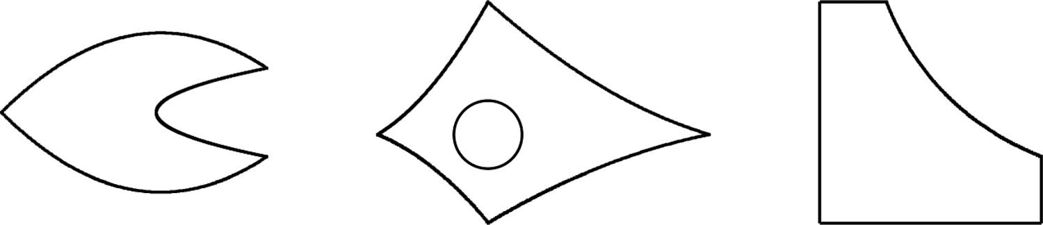
Domains (shaded) with positive reach

Next we introduce a new concept on domains of interest. Let B(0, ϵ) be the closed ball centering at 0 with radius ϵ > 0, and let K^c stand for the complement of the set K in ${ℝ}^n$. For any ϵ > 0, the set

$$E_{ϵ}(K):={\left(K^c+B(0,ϵ)\right)}^c\subset K$$ (1.3)

is called an ϵ-erosion of K.

Definition 1.2

A set $K\subset {ℝ}^n$ is said to have a uniformly positive reach r₀ if there exists some ϵ₀ > 0 such that for all ϵ ∈ [0, ϵ₀], E_ϵ(K) has a positive reach at least r₀.

It is easy to check that any closed convex set has an uniformly positive reach. Indeed, any ϵ-erosion of a convex set is also a closed convex set. Also, a domain with C² boundary has a uniformly positive reach. One can see that each of the three sets in Figure 1 has a uniformly positive reach.

Next let us give an example to show that a set K has a positive reach, but not a uniformly positive reach.

Example 1.3

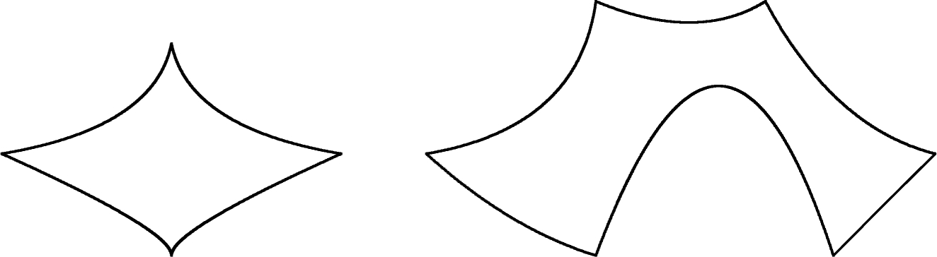
Consider the closed set (on the left) in Figure 2. The set has a positive reach. However, at one of the boundary points, the center of the circle in red in Figure 2 violates the definition of the uniformly positive reach. As shown in Figure 2, the set E_ϵ(K) in red is an ϵ-erosion of K. As ϵ → 0, the boundary of E_ϵ(K) is getting close to the boundary of K. The reach of E_ϵ(K) will go to 0. That is why K does not have a uniformly positive reach.

Figure 2.

The set K on the left (in-between the square and the circle) has a positive reach, but does not have uniformly positive reach. The graph (on right) shows the set K (in blue), its ϵ-erosion E_ϵ(K) (in red), and a small circle (in red). As ϵ becomes smaller, the reach of E_ϵ(K) gets smaller.

In addition, from the definition of the uniformly positive reach, we can see that if a bounded domain $\Omega \subset {ℝ}^n$ has a uniformly positive reach, then Ω is of positive reach as the ϵ-erosions of Ω converge to Ω. Thus, if a domain does not have a positive reach, it can not be of uniformly positive reach.

The main purpose of this paper is to establish the following

Theorem 1.4

Let $\Omega \subset {ℝ}^n$ be a bounded domain. Suppose the closure of Ω is of uniformly positive reach r_Ω. For any f ∈ L²(Ω), let $u\in H_0^1(\Omega )$ be the unique weak solution of the Dirichlet problem:

$$\{\begin{array}{ll}-\Delta u=f,\hfill & in\Omega \hfill \\ u=0,\hfill & on\partial \Omega .\hfill \end{array}$$ (1.4)

Then u ∈ H²(Ω) in the sense that

$$\sum _{i,j=1}^n{\int }_{\Omega }{\left(\frac{{\partial }^2}{\partial x_i\partial x_j}u\right)}^2\le C_0{\int }_{\Omega }{(f)}^{2}dx$$ (1.5)

for a positive constant C₀ dependent on r_Ω, but independent of f and u.

We comment that the domain does not have to be a Lipschitz domain to have the H² regularity based on Theorem 1.4. To see this, we can look at the domain in the middle graph of Figure 1 and image that at one of the four tips, the two boundary curves have the same tangent line, and hence the domain is not Lipschitz. By Theorem 1.4, this domain has the H² regularity. Thus, a domain does not need to have a Lipschitz boundary in order to have the H² regularity.

Next we explain that the assumption of positive reach in Theorem 1.4 is necessary. An example is the solution u = (1 − r²)r^2/3 sin(2θ/3) of the Poisson equation (1.4) over a domain Ω = {(r, θ) : 0 < r < 1, 0 < θ < 2π/3}, where $r=\sqrt{x^2+y^2}$ and θ = arctan(y/x). It is easy to see that u is the solution of a Poisson equation with zero boundary and a uniform bounded function f = 4(2/3 + 1)r^2/3 sin(2θ/3) ∈ L²(Ω) satisfying (1.4). One can check that u is not H²(Ω), see, e.g. [4]. Also see [14] for another example. It is easy to see that the closure of the domain above does not have a positive reach nor uniform positive reach. For the higher dimensional setting, when a bounded domain has a sharp inward cusp, e.g. the well-known Lebesgue spine, the Dirichlet problem has no classic solution. For example, when n = 3, consider the following domain

$$\Omega =\left\{(x,y,z)\in {ℝ}^3:x^2+y^2+z^2<1,x^2+y^2>{\text{e}}^{-1/(2z)}\text{if}z>0\right\}.$$ (1.6)

The inward cusp at (0, 0, 0) is called a Lebesgue spine. At this cusp, the domain does not have a positive reach, and the corresponding solution does not have H² regularity. That is, in order to have H² regularity, the domain must have a positive reach.

Nevertheless, with some extra assumptions on the domain, one indeed may replace the assumption of uniform positive reach by simply positive reach. In particular, we will see in the next section that the conclusion of Theorem 1.4 remains true if Ω is star-shaped and the closure of Ω is of positive reach.

Before proving Theorem 1.4, let us review some classic results on the H² regularity property of the solution to Dirichlet problem of the Poisson equation first. In [15], the concept of domain with a cusp was introduced which is called turning points in [13]. An example from [13] was shown in Figure 3.

Figure 3.

Domain with a turning point [13]

The following result was established in [13]. See also some similar result in [15].

Theorem 1.5

Let f ∈ L²(Ω). Then there exists a unique $u\in H^2(\Omega )\cap H_0^1(\Omega )$ satisfying (1.4) provided

$$\text{lim}\underset{x\to 0}{\text{sup}}\frac{\left(\left|{\varphi }_1^{\prime \prime }(x)\right|+\left|{\varphi }_2^{\prime \prime }(x)\right|\right)\left({\varphi }_2(x)-{\varphi }_1(x)\right)}{{\left({\varphi }_2^{\prime }(x)-{\varphi }_1^{\prime }(x)\right)}^2}<2.$$ (1.7)

with the assumption that 0 is a turning point, where ϕ₁, ϕ₂ are indicated in Figure 3.

As explained in [13], when ϕ₁(x) ≡ 0 and ϕ₂(x) = x^α with α > 1, the sufficient condition in (1.7) is satisfied. However, when ϕ₁(x) ≡ 0 and ϕ₂(x) = x²/4, the sufficient condition (1.7) will not be fulfilled. Nevertheless, we can see that a domain with such a turning point as in Figure 3 has a uniformly positive reach and hence, our Theorem 1.4 can be used to establish the H² regularity even ϕ₂(x) = x²/4. That is, the condition in Theorem 1.4 is more general.

We next recall the following

Theorem 1.6 (Adolfsson, 1992 [1])

Suppose that Ω is a uniformly Lipschitz domain in ${ℝ}^n$ of finite width. If Ω satisfies an outer ball condition of uniform radius, then the unique solution $u\in H_0^1(\Omega )$ of the Dirichlet problem (1.4) has all its second order derivatives in L²(Ω), i.e., u ∈ H²(Ω).

The outer ball condition mentioned above is that at each point p on ∂Ω there exists an exterior ball B, i.e. B ⊂ Ω^c of radius r touch at p, i.e. tangent to ∂Ω, where Ω^c stands for the complement of Ω. When Ω is bounded, Ω is of finite width. When Ω is a bounded Lipschitz domain, it is a uniformly Lipschitz domain. These explain all the notational questions in Theorem 1.6. It is easy to see that any convex domain satisfies the uniform outer ball condition. Also, a convex domain is a Lipschitz domain [2]. Thus, Theorem 1.6 is applicable to convex domains. Recently, the Lipschitz domains satisfying a uniform exterior ball condition is called semi-convex domains (e.g. [24] and [9]).

We will show that when $\overline{\Omega }$ is of positive reach, Ω satisfies an outer ball condition for a uniform radius as explained in Lemma 2.1 (see the following section). On the other hand, if Ω satisfies a uniform outer ball condition, $\overline{\Omega }$ may not have a uniformly positive reach. See the domain in the left panel of Figure 2. (Note that the domain is not Lipschitz. Both Theorems 1.4 and 1.6 fail to establish the regularity for such a domain.) These show that our condition and the one in Theorem 1.6 are two different conditions to ensure the H² regularity of the solution to Dirichlet problem.

Let us also note that if a set $K\subset {ℝ}^m\subset {ℝ}^n$ is of positive reach in ${ℝ}^n$, then it is also of positive reach in ${ℝ}^m$ for m < n. This is not the case for the outer ball condition: indeed, any planar set satisfies a uniform outer ball condition of any radius in ${ℝ}^3$. Let us also emphasize that the main difference between Theorems 1.4 and 1.6 is that in Theorem 1.4, the domain Ω does not need to have a Lipschitz boundary.

Because a set Ω satisfies an outer ball condition for a uniform radius whenever $\overline{\Omega }$ is of positive reach (Lemma 2.1) we may simply replace the outer ball condition in Theorem 1.6 by the positive reach condition, and restate the result as a part of Theorem 1.7. The other part of Theorem 1.7 is a precise relation of the constant C₀ in (1.5) with the positive reach r_Ω of $\overline{\Omega }$.

Theorem 1.7

Suppose that $\Omega \subset {ℝ}^n$ is a bounded domain with Lipschitz boundary. Suppose that the closure of Ω has a positive reach r_Ω > 0. For any f ∈ L²(Ω), let $u\in H_0^1(\Omega )$ be the unique weak solution of the Dirichlet problem (1.4). Then u ∈ H²(Ω) in the sense of (1.5). Moreover, the constant in (1.5) depends only on the positive reach r_Ω.

In Section 2, we first use the concept of star-shaped domain to establish a proof of H² regularity over a star-shaped domain which has a positive reach. See Theorem 2.7. Then, we devote our effort to proving Theorem 1.4. In Section 3.1, we address two applications of the new H² regularity condition.

2. Proofs

We shall prove Theorem 1.7 before proving Theorem 1.4. Let us begin with some properties of sets with positive reach.

Lemma 2.1

Let Ω be a bounded domain in ${ℝ}^n$. If $\overline{\Omega }$ is of positive reach r_Ω, then the following are true:

1. For every 0 < r < r_Ω, and every $y\in {ℝ}^n$ with $\text{dist}(y,\overline{\Omega })<r_{\Omega }$, if x is the projection of y onto $\overline{\Omega }$, then, the closed ball B(z, r) centering at z with radius r intersects $\overline{\Omega }$ precisely at x, where

   $$z=x+\frac{r}{\Vert y-x\Vert }(y-x).$$ (2.1)

2. For every 0 < r < r_Ω, every point on the boundary of Ω is touchable by a closed ball of radius r from outside, that is, for every 0 < r < r_Ω and every x₀ ∈ ∂Ω, there exists a $w\in {ℝ}^n$ such that the closed ball B(w, r) intersects $\overline{\Omega }$ precisely at x₀.

Proof

We prove (i) by contradiction. Suppose (i) is false, then there exist a $y\in {ℝ}^n$ with 0 < dist(y, Ω) < r_Ω, and an $x\in \overline{\Omega }$ with ‖y − x‖ = dist(y, Ω), and 0 < r < r_Ω such that the closed ball B(z, r) does not intersect $\overline{\Omega }$ uniquely at x with z in (2.1). Since $\overline{\Omega }$ is of positive reach, we must have

$$\Vert z-x\Vert >\text{dist}(z,\Omega ).$$ (2.2)

This implies that

$$0<1\le \tau :=\text{sup}\{t:\text{dist}(x+t(y-x),\overline{\Omega })=t\Vert (y-x)\Vert \}\le \frac{r}{\Vert y-x\Vert }<\infty .$$

We have

$$r=\text{dist}(z,x)=\Vert \frac{r}{\Vert y-x\Vert }\cdot (y-x)\Vert \ge \tau \Vert y-x\Vert \ge r_{\Omega }$$

by applying (6) of Theorem 4.8 in Federer [11]. This contradicts to the assumption r < r_Ω. Hence, (i) is proved.

Now, we use (i) to prove (ii). Because x₀ is on the boundary of Ω, there exists N₀ > 0 such that for every integer m ≥ N₀, we can choose a point y_m outside $\overline{\Omega }$ so that ‖y_m − x₀‖ < r/m. Let x_m be the projection of y_m onto $\overline{\Omega }$. Let

$$w_m=x_m+\frac{r}{\Vert y_m-x_m\Vert }\left(y_m-x_m\right).$$

By i), the closed ball B(w_m, r) intersects $\overline{\Omega }$ precisely at x_m. Since

$$\Vert w_m-x_0\Vert \le \Vert w_m-x_m\Vert +\Vert x_m-x_0\Vert \le (1+1/m)r$$

for all m ≥ N₀, the sequence {w_m} is bounded in ${ℝ}^n$. Hence it contains a subsequence that converges to some $w_0\in {ℝ}^n$. Clearly, we have

$$\Vert w_0-x_0\Vert =r=\text{dist}\left(w_0,\overline{\Omega }\right).$$

Since r < r_Ω, the closed ball B(w₀, r) intersects $\overline{\Omega }$ precisely at x₀. This finishes the proof of (ii). □

We are now ready to establish the first part of Theorem 1.7. By using part (ii) of Lemma 2.1 above, we can see the positive reach r_Ω implies the outer ball condition of uniform radius r_Ω in Theorem 1.6. Thus, the first part of Theorem 1.7 is established by Theorem 1.6. We shall continue the investigation of the second part of Theorem 1.7 in the next. The proof is the same as the one for Theorem 1.4. We leave it to when we prove Theorem 1.4.

We now investigate how large the constant C₀ in (1.5) is. We shall connect it to the positive reach r_Ω. To do so, we shall use the following standard formula [13, Theorem 3.1.1.1]: Suppose that $u\in H^2(\Omega )\cap H_0^1(\Omega )$ over a bounded domain $\Omega \subset {ℝ}^n$ with C^{1, 1} smooth boundary. Then we have

$$\begin{gathered} {\int }_{\Omega }|\text{div}v{|}^{2}dx-\sum _{i,j=1}^n{\int }_{\Omega }{\partial }_i{v}_j{\partial }_j{v}_{i}dx \\ =-2{\int }_{\partial \Omega }{v}_T{\nabla }_T(v\cdot n)d\sigma -{\int }_{\partial \Omega }\left[\mathcal{B}\left(v_T,v_T\right)+\text{tr}(\mathcal{B}){(v\cdot n)}^2\right], \end{gathered}$$ (2.3)

where $\mathcal{B}$ is a symmetric matrix of size (n − 1) × (n − 1), tr is the trace operator of the bilinear form: $\text{tr}(\mathcal{B})=-{\sum }_{i=1}^{n-1}\frac{\partial n}{\partial s_i}\cdot {\tau }_i$, and T = [τ₁, …, τ_n−1] and n are the tangent vectors and the outward normal direction vector of ∂Ω, respectively. Letting v = ∇u in (2.3) leads to

$$\begin{gathered} \sum _{i,j=1}^n{\int }_{\Omega }{\left(\frac{{\partial }^2}{\partial x_i\partial x_j}u\right)}^2={\int }_{\Omega }{(\Delta u)}^{2}dx+2{\int }_{\partial \Omega }{\nabla }_{T}u{\nabla }_T(\nabla u\cdot n)d\sigma \\ +{\int }_{\partial \Omega }\left[\mathcal{B}\left({\nabla u|}_T,{\nabla u|}_T\right)+\text{tr}(\mathcal{B}){(\nabla u\cdot n)}^2\right]d\sigma . \end{gathered}$$ (2.4)

See a detailed proof of (2.4) in [13] or [5]. When the underlying domain Ω is convex, we have $\text{tr}(\mathcal{B})\le 0$ and $\mathcal{B}\left(v_T,v_T\right)\le 0$. Thus we have C₀ = 1 in (1.5). We can also use the so-called Miranda–Talenti estimate. In [22] and [27] the following equality was calculated: for any u ∈ H²(Ω),

$${\int }_{\Omega }\sum _{i,j=1}^n\left(\frac{{\partial }^{2}u}{\partial x_i^2}\frac{{\partial }^{2}u}{\partial x_j^2}-{\left(\frac{{\partial }^{2}u}{\partial x_i\partial x_j}\right)}^2\right)dx=-(n-1){\int }_{\partial \Omega }H(x)\Vert \nabla u{\Vert }^{2}d\sigma ,$$ (2.5)

where H(x) is the mean curvature of ∂Ω which is C² boundary. In the setting of the convex domain Ω, H(x) is non-positive, we use (2.5) and the following identity:

$$\sum _{i,j=1}^n{\left(\frac{{\partial }^{2}u}{\partial x_i\partial x_j}\right)}^2+\sum _{i,j=1}^n\left(\frac{{\partial }^{2}u}{\partial x_i^2}\frac{{\partial }^{2}u}{\partial x_j^2}-{\left(\frac{{\partial }^{2}u}{\partial x_i\partial x_j}\right)}^2\right)={(\Delta u)}^2$$ (2.6)

to conclude the inequality in (1.5) with C₀ ≡ 1. When the domain Ω has a positive reach r_Ω, the mean curvature H(x) at each x can be bounded above by (n−1)/r_Ω. This is quantitatively established in the following lemma.

Lemma 2.2

Suppose that Ω is a bounded open set with C^{1, 1} boundary ∂Ω. Suppose that $\text{tr}(\mathcal{B})\le c$ for a fixed real number c > 0, e.g. c = (n − 1)/r over ∂Ω. Then the inequality in (1.5) holds for a constant C₀ = (1 + (cK)²C²)/(1 – cKϵ), where C is a constant in the Poincaré inequality (2.7) and K is the constant in the trace inequality in (2.10).

Proof

Using Poincaré inequality, we have

$$\Vert u{\Vert }_{L^2(\Omega )}\le C\Vert \nabla u{\Vert }_{L^2(\Omega )}$$ (2.7)

for a positive constant C dependent only on the size of Ω. As u is a weak solution, we have

$${\int }_{\Omega }|\nabla u{|}^{2}dx=-{\int }_{\Omega }(\Delta u)udx.$$

We use Cauchy–Schwarz inequality to get

$$\Vert u{\Vert }_{L^2(\Omega )}^2\le C^2\Vert \nabla u{\Vert }_{L^2(\Omega )}^2\le C^2\Vert \Delta u{\Vert }_{L^2(\Omega )}\Vert u{\Vert }_{L^2(\Omega )}.$$

That is, we have

$$\Vert u{\Vert }_{L^2(\Omega )}\le C^2\Vert \Delta u{\Vert }_{L^2(\Omega )}$$ (2.8)

and

$$\Vert \nabla u{\Vert }_{L^2(\Omega )}\le C\Vert \Delta u{\Vert }_{L^2(\Omega )}.$$ (2.9)

In addition, we need the standard Sobolev trace inequality:

$${\int }_{\partial \Omega }|u{|}^{2}d\sigma \le K\left(ϵ{\int }_{\Omega }|\nabla u{|}^{2}dx+\frac{1}{ϵ}{\int }_{\Omega }|u{|}^{2}dx\right)$$ (2.10)

for any ϵ ∈ (0, 1), where K > 0 is a constant independent of u. The second term in (2.4) can be estimated by

$${\int }_{\partial \Omega }\text{tr}(\mathcal{B}){(\nabla u\cdot n)}^{2}d\sigma \le c{\int }_{\partial \Omega }{(\nabla u\cdot n)}^{2}d\sigma \le c\Vert \nabla u{\Vert }_{L^2(\partial \Omega )}^2.$$

We then use the trace inequality to the right-hand side of the above inequality to get

$$c\Vert \nabla u{\Vert }_{L^2(\partial \Omega )}^2\le cKϵ\sum _{i,j=1}^n{\int }_{\Omega }{\left(\frac{{\partial }^2}{\partial x_i\partial x_j}u\right)}^2+\frac{cK}{ϵ}{\int }_{\Omega }|\nabla u{|}^{2}dx.$$ (2.11)

Indeed, we first consider an open set V_ϵ ⊂ Ω with C^{1, 1} boundary. Using the interior regularity of u, we have the above inequality with Ω replaced by V. Then we let V_ϵ → Ω to have (2.11).

Returning to (2.4), we have

$$\sum _{i,j=1}^n{\int }_{\Omega }{\left(\frac{{\partial }^2}{\partial x_i\partial x_j}u\right)}^2\le {\int }_{\Omega }{(\Delta u)}^{2}dx+cKϵ\sum _{i,j=1}^n{\int }_{\Omega }{\left(\frac{{\partial }^2}{\partial x_i\partial x_j}u\right)}^2+\frac{cK}{ϵ}{\int }_{\Omega }|\nabla u{|}^{2}dx$$

By choosing ϵ = 1/(cK) < 1 and using (2.9),

$$(1-ϵcK)\sum _{i,j=1}^n{\int }_{\Omega }{\left(\frac{{\partial }^2}{\partial x_i\partial x_j}u\right)}^2\le {\int }_{\Omega }{(\Delta u)}^{2}dx+{(cK)}^2{C}^2{\int }_{\Omega }{(\Delta u)}^{2}dx.$$

The desired inequality (1.5) follows with C₀ = (1 + (cK)²C²)/(1 – cKϵ).□

Let us make a remark that the result in the lemma above is not new. A similar result can be found in [18]. That is, when the domain with boundary ∂Ω consists of piecewise C² smooth surfaces with curvature bounded below by a constant c > 0, one has the property (1.5). See [18, Lemma 8.1]. When the domain Ω has a positive reach, we can estimate c in terms of the reach r = reach(Ω) as in the following lemma.

Lemma 2.3

Let Ω be a bounded set in ${ℝ}^n$ with a C^{1, 1} boundary. Suppose that the closure of Ω has a positive reach. If reach(Ω) ≥ r, then $\text{tr}(\mathcal{B})\le \frac{n-1}{r}$.

Proof

Let Γ be the boundary of Ω. For any point P on Γ, we choose a coordinate system {y₁, y₂, …, y_n} with origin at P such that the hyperplane y_n = 0 is tangent to Γ at P, and choose a rectangular box

$$V=\left\{\left(y_1,y_2,\dots ,y_n\right):-a_j\le y_j\le a_j,1\le j\le n\right\},$$

and a function ϕ of class C^{1, 1} in the closure of

$$V^{\prime }=\left\{\left(y_1,y_2,\dots ,y_{n-1}\right):-a_j\le y_j\le a_j,1\le j\le n-1\right\},$$

such that $\left|\varphi \left(y_1,y_2,\dots ,y_{n-1}\right)\right|\le \frac{a_n}{2}$ for every (y₁, y₂, …, y_n−1) ∈ V′, and

$$\begin{gathered} \Omega \cap V=\left\{\left(y_1,y_2,\dots ,y_n\right)\in V:y_n\le \varphi \left(y_1,\dots ,y_{n-1}\right)\right\}, \\ \Omega \cap \Gamma =\left\{\left(y_1,y_2,\dots ,y_n\right)\in V:y_n=\varphi \left(y_1,\dots ,y_{n-1}\right)\right\}. \end{gathered}$$

Then,

$$\text{tr}\left(\mathcal{B}\right)=\sum _{j=1}^{n-1}\frac{{\partial }^2\varphi }{\partial y_i^2}\left(0,0,\dots ,0\right).$$

Note that by Lemma 2.1, for any δ < r, there exists a ball of radius δ which intersects Ω only at the point P. Because the hyperplane y_n = 0 is the tangent plane of Ω at the origin P, this ball must lie entirely above the tangent hyperplane y_n = 0. Consequently, for |h| < min{a₁, δ}, we have $\varphi \left(h,0,\dots ,0\right)\le \delta -\sqrt{{\delta }^2-h^2}$. Since ϕ(0, …, 0) = 0 and $\frac{\partial \varphi }{\partial y_1}\left(0,\dots ,0\right)=0$, we obtain

$$\begin{gathered} \frac{{\partial }^2\varphi }{\partial y_1^2}\left(0,\dots ,0\right)=\underset{h\to 0}{\text{lim}}\frac{\varphi \left(h,0,\dots ,0\right)+\varphi \left(-h,0,\dots ,0\right)}{h^2} \\ \le \underset{h\to 0}{\text{lim}}\frac{2\delta -2\sqrt{{\delta }^2-h^2}}{h^2} \\ =\frac{1}{\delta }. \end{gathered}$$

Similarly, we have $\frac{{\partial }^2\varphi }{\partial y_j^2}\left(0,\dots ,0\right)\le \frac{1}{\delta }$ for all 2 ≤ j ≤ n − 1. Because δ < r is arbitrary, the statement of the lemma follows. □

Combining the results above, we obtain the following:

Corollary 2.4

Let Ω be a bounded set in ${ℝ}^n$ with a C^{1, 1} boundary. Suppose that $\overline{\Omega }$ has a positive reach(Ω) ≥ r. Then

$$\sum _{i,j=1}^n{\int }_{\Omega }{\left(\frac{{\partial }^2}{\partial x_i\partial x_j}u\right)}^2\le C_1{\int }_{\Omega }{\left(\Delta u\right)}^{2}dx$$ (2.12)

for a constant C₁ = (1 + ((n − 1)K/r)²C²)/(1 – ϵ(n – 1)K/r), where C is the Poincaré constant in (2.7) and K is the constant in the trace inequality in (2.10).

Next we extend Theorem 1.7 to a more general setting. In particular, we need to remove the assumption of C^{1, 1} boundary in Corollary 2.4. Let us start with a well-known concept of star-shaped domains [4]. See Figure 4 for such an example.

Figure 4.

Left: A star-shaped domain which is not Lipschitz at one corner (the bottom one). Right: A multi-star shaped domain with uniform positive reach

Definition 2.5

Let $\Omega \subset {ℝ}^n$ be a bounded domain. We say Ω is a star-shaped domain if there exists a point, say x₀ ∈ Ω such that the line segment from x₀ to any point x ∈ Ω is completely contained in Ω. x₀ is called the center of Ω.

Clearly, we can extend the definition of star-shaped domains to the following way.

Definition 2.6

Let $\Omega \subset {ℝ}^n$ be a bounded domain. We say Ω is a multiple-star-shaped domain if there exist finitely many points, say x₁, …, x_k ∈ Ω such that for any point x ∈ ∂Ω, there exists an index i ∈ {1, …, k} such that the line segment [x, x_i] is completely contained in Ω. x₁, …, x_k are called the centers of Ω.

Typically, a bounded domain with Lipschitz boundary is a multiple-star-shaped domain. A multiple-star-shaped domain may have a uniformly positive reach. See Figure 4 for an example.

We now state the H² regularity of the solution to the Dirichlet problem of Poisson equations over a general domain.

Theorem 2.7

Suppose that $\Omega \subset {ℝ}^n$ is a bounded a star-shaped domain. Suppose that the closure of Ω is of positive reach r. For any f ∈ L²(Ω), let $u\in H_0^1\left(\Omega \right)$ be the unique weak solution of the Dirichlet problem (1.4). Then u ∈ H²(Ω) satisfies (1.5) with constant C₀ dependent on r.

To prove the above theorem, we need a few preparatory results. The lemma below shows that for any ϵ > 0 there is an open subset U_ϵ ⊃ Ω such that U_ϵ has a C^{1, 1} smooth boundary and dist(U_ϵ, Ω) < ϵ.

Lemma 2.8

If $\Omega \subset {ℝ}^n$ is of positive reach r₀ = reach(Ω), then for any 0 < ϵ < r₀, the boundary of Ω_ϵ := Ω + B(0, ϵ) containing Ω is of C^{1, 1}. Furthermore, Ω_ϵ has a positive reach ≥ r₀ − ϵ.

Proof

Because the boundary B(0, ϵ) is of C^∞, it is known (see [16]) that the boundary of Ω_ϵ is of C^{1, 1} if Ω is convex. We now extend the result to the setting that Ω is a domain whose closure has a positive reach.

For any x ∈ ∂Ω_ϵ, there exists y ∈ ∂Ω such that ‖x − y‖ = dist(x, Ω) = ϵ since Ω is of positive reach and ϵ < r₀. Also, for any ϵ < r < r₀, there exists a closed ball of radius r that intersects Ω only at y. Denote this ball by B(c, r). Then the ball B(c, r − ϵ) intersects Ω_ϵ only at x.

On the other hand, the closed ball B(y, ϵ) is contained in ${\overline{\Omega }}_{ϵ}$ and intersect ∂Ω_ϵ only at x. Hence, ∂Ω_ϵ intersects two tangent balls B(y, ϵ) and B(c, r − ϵ) at x. Without loss of generality, we may assume x = 0 and the tangent hyperplane at 0 is x_n = 0, where x = (x₁, …, x_n). The boundary of Ω_ϵ can be expressed as x_n = ϕ(x₁, …, x_n−1) by the implicit function theorem. Note that ϕ(0, 0, …, 0) = 0. Letting $\overline{x}=\left(x_1,\dots ,x_{n-1}\right)$ be the first part of x ∈ ∂Ω, for $\Vert \overline{x}\Vert <\text{min}\{ϵ,r-ϵ\}$, we have

$$\sqrt{{ϵ}^2-{\Vert \overline{x}\Vert }^2}-ϵ\le \varphi \left(\overline{x}\right)=\varphi \left(x_1,x_2,\dots ,x_{n-1}\right)\le r-ϵ-\sqrt{{\left(r-ϵ\right)}^2-{\Vert \overline{x}\Vert }^2}.$$ (2.13)

We claim that ϕ is differentiable at 0. Indeed, we have

$$\frac{\varphi (\overline{x})-\varphi (0)}{\Vert \overline{x}\Vert }\le \frac{r-ϵ-\sqrt{{(r-ϵ)}^2-{\Vert \overline{x}\Vert }^2}}{\Vert \overline{x}\Vert }=\frac{\Vert \overline{x}\Vert }{r-ϵ+\sqrt{{(r-ϵ)}^2-{\Vert \overline{x}\Vert }^2}}$$ (2.14)

and

$$\frac{\varphi (\overline{x})-\varphi (0)}{\Vert \overline{x}\Vert }\ge -\frac{\Vert \overline{x}\Vert }{ϵ+\sqrt{{ϵ}^2-{\Vert \overline{x}\Vert }^2}}$$ (2.15)

by using the inequalities in (2.13). It follows that ϕ is differentiable at 0 and ∇ϕ(0) = 0. Similar analysis for all point in Ω implies that Ω has a C¹ boundary.

We next claim that the gradient of ϕ is bounded from above and below. Using the notations above, we have

$$\frac{\varphi (\overline{x})+\varphi (-\overline{x})-\varphi (0)}{2{\Vert \overline{x}\Vert }^2}\le \frac{r-ϵ-\sqrt{{(r-ϵ)}^2-{\Vert \overline{x}\Vert }^2}}{{\Vert \overline{x}\Vert }^2}=\frac{1}{r-ϵ+\sqrt{{(r-ϵ)}^2-{\Vert \overline{x}\Vert }^2}}$$ (2.16)

and similarly,

$$\frac{\varphi (\overline{x})+\varphi (-\overline{x})-\varphi (0)}{2{\Vert \overline{x}\Vert }^2}\ge -\frac{1}{ϵ+\sqrt{{ϵ}^2-{\Vert \overline{x}\Vert }^2}}.$$ (2.17)

Therefore, for all $\Vert \overline{x}\Vert \le \text{min}\{r-ϵ,ϵ\}$, we have

$$-\frac{1}{ϵ}<\frac{\varphi (\overline{x})+\varphi (-\overline{x})-2\varphi (0)}{2{\Vert \overline{x}\Vert }^2}<\frac{1}{r-ϵ}.$$ (2.18)

We now apply a known result Lemma 2.9 to finish the proof of C^{1, 1}.

Finally, we show Ω is of reach r − ϵ. For any point $q\notin {\Omega }_{ϵ}$, if dist(q, Ω_ϵ) < r − ϵ, we know dist(q, Ω) = δ < r. Since the reach of Ω is at least r, there exists a closed ball centering at q with radius δ > 0 which intersects Ω only at one point p, say. Now the closed ball centered at q with radius δ − ϵ intersects Ω_ϵ only at one point, namely the point p + ϵ(q − p)/δ. Therefore, Ω_ϵ is of reach δ − ϵ. This holds for all δ < r. Thus, Ω_ϵ has a reach of δ − ϵ. In general, r − ϵ is the best one can hope for. Indeed, if Ω is the complement of an open ball with radius r which has a positive reach r, then Ω_ϵ is the complement of an open ball with radius r − ϵ which has a reach r − ϵ. □

Lemma 2.9

Assume that the function f is bounded on a neighborhood of x₀ ∈ ∂Ω. f is of class C^{1, 1} at x₀ if and only if there exists a neighborhood U of x₀ such that the central difference

$${\Delta }_{2}f\left(x;h\right)=f\left(x+hd\right)-2f\left(x\right)+f\left(x-hd\right)$$ (2.19)

is bounded on U for all h ∈ (−δ, δ) for a fixed δ > 0 and $d\in {\mathcal{S}}^{n-1}$ which is the unit sphere in ${ℝ}^n$.

Proof

See [29, Corollary 2.1] for a proof. □

Next we show that if Ω is a star-shaped domain whose closure is of positive reach, then for any ϵ > 0, there exists an open set U_ϵ ⊂ Ω with C^{1, 1} boundary with dist(Ω, U_ϵ) ≤ ϵ.

Lemma 2.10

Let Ω be a bounded domain with a positive reach in ${ℝ}^n$. Suppose that Ω is a star-shaped domain. Then, for each ϵ > 0, there exists an open set U with C^{1, 1} smooth boundary such that U_ϵ ⊂ Ω and dist(Ω, U_ϵ) ≤ ϵ.

Proof

Let x₀ ∈ Ω be the center of the star-shaped domain Ω. By Lemma 2.8, we have Ω_ϵ containing Ω with C^{1, 1} boundary for any ϵ < r, where r stands for the reach of Ω. Letting ∂Ω_ϵ be the boundary of Ω_ϵ, we define

$$U_{ϵ}=\left\{y=x_0+t\left(x-x_0\right):0\le t\le \left(1-\frac{2ϵ}{\Vert x-x_0\Vert }\right),x\in \partial {\Omega }_{ϵ}\right\}.$$ (2.20)

We claim that U_ϵ ⊂ Ω is a domain with C^{1, 1} boundary. Indeed, at the center x₀ ∈ Ω, we fix a spherical coordinate system. For any point x ∈ ∂Ω_ϵ, we define a function ϕ of the angle of the ray from x₀ to x with value to be the length ‖x – x₀‖. Then ϕ is a function describing the boundary of Ω_ϵ. Since Ω_ϵ has a C^{1, 1} boundary by Lemma 2.8, ϕ is a C^{1, 1} function. Next we define a new function ψ over the same spherical coordinate system as ϕ by

$$\psi \left(x_0+\left(1-\frac{2ϵ}{\Vert x-x_0\Vert }\right)\left(x-x_0\right)\right)=\varphi \left(x\right),\forall x\in {\Omega }_{ϵ}$$

which is the function which can describe the boundary of U_ϵ. Clearly, ψ(x) is a C^{1, 1} function for x ∈ U_ϵ and hence, U_ϵ has a C^{1, 1} boundary. □

We are now ready to prove Theorem 2.7 under an assumption that Ω is a star-shaped domain.

Proof of Theorem 2.7

We use Lemma 2.10 to select a sequence of sets U_ϵ ⊂ Ω with dist(Ω, U_ϵ) ≤ ϵ with ϵ → 0.

For a function f ∈ L²(Ω). Then, we define $u_{ϵ}\in H_0^1\left(U_{ϵ}\right)$ to be the weak solution of

$$\{\begin{array}{cc}-\Delta u=f,\hfill & \text{in }{U}_{ϵ},\hfill \\ u=0,\hfill & \text{on }\partial U_{ϵ}.\hfill \end{array}$$ (2.21)

We claim that u_ϵ ∈ H²(U_ϵ). Indeed, using Lemma 2.10 again, we take an open set V_η ⊂ U_ϵ. The interior regularity of [10] and the C^{1, 1} boundary of V_η allows us to have

$$\begin{gathered} \sum _{i,j=1}^n{\int }_{V_{\eta }}{\left(\frac{{\partial }^2}{\partial x_i\partial x_j}{u}_{ϵ}\right)}^2={\int }_{V_{\eta }}{f}^{2}dx+{\int }_{\partial V_{\eta }}{\nabla }_T{u}_{ϵ}{\nabla }_T\left(\nabla u_{ϵ}\cdot n\right)d\sigma \\ +{\int }_{\partial V_{\eta }}\left[\mathcal{B}\left({\nabla u_{ϵ}|}_T,{\nabla u_{ϵ}|}_T\right)+\text{tr}\left(\mathcal{B}\right){\left(\nabla u_{ϵ}\cdot n\right)}^2\right]d\sigma \end{gathered}$$ (2.22)

by using (2.4), where T and n stand for the tangential and normal direction of ∂V_η. As the above equation in (2.22) holds for all V_η, hence it holds for U_ϵ. Using the boundary condition u_ϵ|∂Ω = 0, we have ∇_Tu_ϵ = 0 and

$$\sum _{i,j=1}^n{\int }_{U_{ϵ}}{\left(\frac{{\partial }^2}{\partial x_i\partial x_j}{u}_{ϵ}\right)}^2={\int }_{U_{ϵ}}{f}^{2}dx+{\int }_{\partial U_{ϵ}}\text{tr}(\mathcal{B}){\left(\nabla u_{ϵ}\cdot n\right)}^{2}d\sigma ,$$ (2.23)

Since the domain U_ϵ has C^{1, 1} boundary and a positive reach, we use Corollary 2.4, i.e. (2.12) to have

$$\sum _{i,j=1}^n{\int }_{U_{ϵ}}{\left(\frac{{\partial }^2}{\partial x_i\partial x_j}{u}_{ϵ}\right)}^2\le C_1\Vert f{\Vert }_{L^2\left(\Omega \right)}^2$$

with C₁ ≥ 1 being a positive constant dependent on the reach.

Let us extend u_ϵ by zero outside U_ϵ to Ω, also denote it by u_ϵ. Then u_ϵ belongs to $H^2(\Omega )\cap H_0^1(\Omega )$ for all ϵ > 0 sufficiently small and

$${\Vert u_{ϵ}\Vert }_{H^2\left(U_{ϵ}\right)}\le C_2{\Vert f\Vert }_{L^2\left(\Omega \right)}$$ (2.24)

for another positive constant C₂. By Rellich’s theorem, there is $\tilde{u}\in H^2(\Omega )$ and a subsequence, without loss of generality, we may assume that $u_{ϵ}\to \tilde{u}$ strongly in L²(Ω), strongly in H¹(Ω), and weakly in H²(Ω).

We now claim that $u\to \tilde{u}$. Since $u\in H_0^1(\Omega )$, for any $\varphi \in C_0^{\infty }(\Omega )$, we have

$${\int }_{\Omega }\nabla u\nabla \varphi dx=-{\int }_{\Omega }f\varphi dx.$$ (2.25)

Since ϕ is compactly supported in Ω, Lemma 2.10 shows that there is ϵ > 0 such that supp(ϕ) ⊂ U_ϵ for all ϵ > 0 sufficiently small. Since $u_{ϵ}\in H^2\left(U_{ϵ}\right)\cap H_0^1\left(U_{ϵ}\right)$ solves the Poisson equation over U_ϵ and $u_{ϵ}\to \tilde{u}$ in $H_0^1(\Omega )$ weakly, we get

$$\begin{gathered} {\int }_{\Omega }\nabla \tilde{u}\nabla \varphi dx={\text{lim}}_{ϵ\to 0_{+}}{\int }_{\Omega }\nabla u_{ϵ}\nabla \varphi dx \\ ={\text{lim}}_{ϵ\to 0_{+}}-{\int }_{U_{ϵ}}f\varphi dx \\ =-{\int }_{\Omega }f\varphi dx \\ ={\int }_{\Omega }\nabla u\nabla \varphi dx \end{gathered}$$ (2.26)

by using (2.25). It follows that $\nabla u\equiv \nabla \tilde{u}$ since (2.26) holds for all $\varphi \in C_0^{\infty }(\Omega )$. Then $u\equiv \tilde{u}$ because of the zero boundary condition for both u and $\tilde{u}$. Therefore, u ∈ H²(Ω).

Remark 2.11

Based on the proof above, we can remove the C^{1, 1} assumption in Corollary 2.4 to have (2.12) when the underlying domain Ω is a star-shaped domain.

Finally let us proceed to establish Theorem 1.4.

Proof of Theorem 1.4

The proof of Theorem 1.4 is similar to that of Theorem 2.7 in the following senses. Indeed, instead of defining U_ϵ ⊂ Ω by using the formula in (2.20), we let E_ϵ(Ω) = (Ω^c + B(0, ϵ))^c ⊂ Ω be an ϵ-erosion of Ω and

$$U_{ϵ}=E_{2ϵ}(\Omega )+B(0,ϵ)\subset \Omega .$$ (2.27)

By the assumption of Theorem 1.4, i.e. the uniformly positive reach, we know the domain E_2ϵ(Ω) has a positive reach r₀ for sufficiently small ϵ. Then by Lemma 2.8, U_ϵ has C^{1, 1} boundary. Then the rest of the proof is the same as that of Theorem 2.7. These finish the proof. □

3. Some Applications

In this section, we apply the new regularity conditions to two examples of PDE and establish the H² regularity.

3.1. The Strong Solution to Second Order PDE in Non-divergence Form

In this section we study the solution to the second order PDE in non-divergence form in (1.1). For simplicity, we let

$$\mathcal{L}\left(u\right)=\sum _{i,j=1}^n{a}_{i,j}\left(x\right)\frac{{\partial }^2}{\partial x_i\partial x_j}u$$ (3.1)

be the differential operator associated with the model problem (1.1). Next we assume that

Definition 3.1

The PDE coefficients a_ij (i, j = 1, …, n) satisfy the Cordés condition [23]:

$$\frac{{\sum }_{i,j=1}^n{a}_{ij}^2}{{\left({\sum }_{i=1}^n{a}_{ii}\right)}^2}\le \frac{1}{n-1+ϵ},in\Omega ,$$ (3.2)

for a positive number ϵ ∈ (0, 1].

Following the studies in [25, 26], and [23], we assume that

$$\gamma =\frac{{\sum }_{i=1}^n{a}_{ii}}{{\sum }_{i,j=1}^n{a}_{ij}^2}>0.$$ (3.3)

For example, the ellipticity of the PDE in (1.1) will imply (3.3) when n = 2. The following result is known.

Lemma 3.2 ([23, 25])

Suppose that the PDE coefficients a_ij, (i, j = 1, …, n) satisfy the Cordés condition. Then

$$\left|\gamma \mathcal{L}\left(u\right)-\Delta u\right|\le \sqrt{1-ϵ}{\left(\sum _{i,j=1}^n{\left(\frac{{\partial }^2}{\partial x_i\partial x_j}u\right)}^2\right)}^{1/2}.$$ (3.4)

With this preparation, we are able to prove one of our main results in this section.

Theorem 3.3

Suppose that Ω has a uniformly positive reach. If the PDE coefficients a_ij satisfy the Cordés condition with an close to 1 such that $\sqrt{(1-ϵ)C_0}<1$, then there exists a unique strong solution u ∈ H²(Ω) to the PDE in (1.1), where C₀ appears in Theorem 1.4, i.e. in (1.5).

Proof

We mainly follow the approach in [25]. First of all, it is easy to see that ${\Vert \Delta u\Vert }_{L^2(\Omega )}$ is a norm on H. By Theorem 1.4, ${\Vert \Delta u\Vert }_{L^2(\Omega )}=0$ implies

$$\sum _{i,j=1}^n{\left(\frac{{\partial }^2}{\partial x_i\partial x_j}u\right)}^2=0$$

by using (1.5). Thus, u is a linear polynomial over Ω. The zero boundary condition of u implies u ≡ 0. The other norming properties can be established in a standard fashion.

Next let us consider an equivalent PDE: find $u\in H^2(\Omega )\cap H_0^1(\Omega )$ satisfying the following:

$$\gamma \mathcal{L}\left(u\right)=\gamma f,\in \Omega .$$ (3.5)

Write $H=H^2(\Omega )\cap H_0^1(\Omega )$ and define a bilinear form [25].

$$A(u,v)={\int }_{\Omega }\gamma \mathcal{L}(u)\Delta vdx$$ (3.6)

We now claim that the bilinear form A(u, v) is continuous in the sense that there is a positive constant β > 0 such that

$$|A(u,v)|\le \beta {\Vert \Delta u\Vert }_{L^2(\Omega )}{\Vert \Delta v\Vert }_{L^2(\Omega )}$$ (3.7)

for all u, v ∈ H and coercive, i.e.

$$A(u,u)\ge \alpha {\Vert \Delta u\Vert }_{L^2(\Omega )}^2,\forall u\in H$$ (3.8)

for ϵ ∈ (0, 1) large enough, where α > 0 is a constant independent of u. Indeed, we use Lemma 3.2 to have

$$\begin{gathered} \left|A(u,u)-{\int }_{\Omega }{\left(\Delta u\right)}^{2}dx\right|\le {\int }_{\Omega }|\gamma \mathcal{L}(u)-\Delta u\Vert \Delta u|dx \\ \le {\int }_{\Omega }\sqrt{1-ϵ}{\left(\sum _{i,j=1}^n{\left(\frac{{\partial }^2}{\partial x_i\partial x_j}u\right)}^2\right)}^{1/2}\left|\Delta u\right|dx \\ \le \sqrt{1-ϵ}{C}_0^{1/2}{\int }_{\Omega }{\left(\Delta u\right)}^{2}dx \end{gathered}$$

by Cauchy–Schwarz inequality and the inequality in (2.12). If ϵ ∈ (0, 1) is large enough such that $\sqrt{C_0}\sqrt{1-ϵ}<1$, we have (3.7) and (3.8) with $\beta =1+\sqrt{1-ϵ}\sqrt{C_0}$ and $\alpha =1-\sqrt{1-ϵ}\sqrt{C_0}$.

Now Lax–Milgram theorem implies that there exists a unique weak solution in H satisfying

$$A(u,v)={\int }_{\Omega }\gamma f\Delta vdx.$$

That is, u is a weak solution in H satisfying (3.5). Since u ∈ H²(Ω), u is a strong solution. This finishes the proof of Theorem 3.3. □

3.2. The Regularity of the Solution to the Helmholtz Problem

We are interested in the regularity of the solution of the following Helmholtz problem:

$$\{\begin{array}{cc}-\Delta u-k^{2}u=f,\hfill & \text{in }\Omega \subset {ℝ}^2\hfill \\ \frac{\partial }{\partial n}u+iku=0,\hfill & \text{on }\partial \Omega ,\hfill \end{array}$$ (3.9)

where Ω is a bounded domain with Lipschitz boundary, $i=\sqrt{-1}$ denotes the imaginary unit, n is the normal to ∂Ω, and k ≥ 1 is the wave number. This Helmholtz problem arises from many application areas: acoustic scattering, electromagnetic fields, etc. In the literature, the solution to Helmholtz problem (3.9) will be H² if Ω is convex or Ω has a C² smooth boundary (see [8]). We now show that the unique solution u is of H² regularity when Ω has a uniform positive reach.

Theorem 3.4

Let $\Omega \subset {ℝ}^n$ be a bounded domain. Suppose the closure of Ω is of uniformly positive reach r_Ω > 0. For any f ∈ L²(Ω), let $u\in H_0^1(\Omega )$ be the unique weak solution of the Helmholtz problem (3.9). Then u ∈ H²(Ω) satisfying (1.5) for a positive constant C₀ dependent on r_Ω, but independent of f and u.

Proof

The ideas for this proof are similar to that of Theorem 1.4. We first prove that the solution u satisfies (1.5) if u ∈ H²(Ω). Then we find a sequence of subdomains U_ϵ ⊂ Ω which has C^{1, 1} boundary with uniform positive reach r_Ω/2 and solve u_ϵ ∈ H²(Ω_ϵ) satisfying (1.5) with a constant C₀ dependent on r_Ω/2. Finally, we use Rellich theorem to find a limit u ∈ H²(Ω) of u_ϵ strongly in L²(Ω) and strong in H¹(Ω) and weakly in H²(Ω).

The major proof is to show the boundedness of u in H²(Ω) semi-norm. Let us start with the the following identity [13]: when Ω has C^{1, 1} boundary and $u\in {ℍ}^2(\Omega )$, u satisfies

$$\begin{gathered} \sum _{i,j=1}^n{\int }_{\Omega }{\left(\frac{{\partial }^2}{\partial x_i\partial x_j}u\right)}^2={\int }_{\Omega }{\left(\Delta u\right)}^{2}dx+{\int }_{\Gamma }{\nabla }_{T}u{\nabla }_T\left(\nabla u\cdot n\right)d\sigma \\ +{\int }_{\Gamma }\left[\mathcal{B}\left({\nabla u|}_T,{\nabla u|}_T\right)+\text{tr}\left(\mathcal{B}\right){\left(\nabla u\cdot n\right)}^2\right]d\sigma \end{gathered}$$ (3.10)

for n ≥ 2, where tr is the standard trace operator, $\mathcal{B}$ is a bilinear form associated with the curvature of boundary surface Γ of Ω as defined in [13], and n is the unit outward normal direction of Γ = ∂Ω and T is the unit tangential direction of Γ.

Since u is the solution of (3.9), we use the boundary condition to get

$${\int }_{\Gamma }{\nabla }_{T}u{\nabla }_T(\nabla u\cdot n)d\sigma =-k{\int }_{\Gamma }{\nabla }_{T}u{\nabla }_{T}ud\sigma =-k{\int }_{\Gamma }{\left|{\nabla }_{T}u\right|}^{2}d\sigma \le 0.$$ (3.11)

Next we split Γ into three portions according the symmetric Hessian matrix $\mathcal{B}$, i.e. Γ = Γ_p ∪ Γ_n ∪ Γ_i such that $\mathcal{B}\ge 0$ for x ∈ Γ_p, $\mathcal{B}<0$ for x ∈ Γ_n and $\mathcal{B}$ is indefinite when x ∈ Γ_i. The last term in (3.10) can be rewritten as

$${\int }_{\Gamma }\left[\mathcal{B}\left({\nabla u|}_T,{\nabla u|}_T\right)+\text{tr}(\mathcal{B}){(\nabla u\cdot n)}^2\right]d\sigma \le {\int }_{{\Gamma }_p\cup {\Gamma }_i}\left[\mathcal{B}\left({\nabla u|}_T,{\nabla u|}_T\right)+\text{tr}(\mathcal{B}){(\nabla u\cdot n)}^2\right]d\sigma .$$

When the underlying domain Ω has a positive reach r_Ω, we have $\text{tr}\left(\mathcal{B}\right)\le (n-1)/r_{\Omega }$ over the boundary Γ by Lemma 2.3. Also, over Γ_p, we $\mathcal{B}\left({\nabla u|}_T,{\nabla u|}_T\right)\le {\Vert \nabla u\Vert }_{\Gamma }^2\Vert \mathcal{B}\Vert \le {\mid \nabla u\Vert }_{\Gamma }^2(n-1)/r_{\Omega }$. Thus,

$${\int }_{{\Gamma }_p}\left[\mathcal{B}\left({\nabla u|}_T,{\nabla u|}_T\right)+\text{tr}(\mathcal{B}){(\nabla u\cdot n)}^2\right]d\sigma \le \frac{n-1}{r_{\Omega }}{\int }_{{\Gamma }_p}\left[{\left|{\nabla u}_T\right|}^2+{(\nabla u\cdot n)}^2\right]d\sigma .$$

Over Γ_i, we rewrite $\mathcal{B}={\mathbb{B}}_p-{\mathbb{B}}_n$ with symmetric nonnegative definite matrices ${\mathbb{B}}_p$ and ${\mathbb{B}}_n$. Thus,

$${\int }_{{\Gamma }_i}\left[\mathcal{B}\left({\nabla u|}_T,{\nabla u|}_T\right)+\text{tr}(\mathcal{B}){(\nabla u\cdot n)}^2\right]d\sigma \le {\int }_{{\Gamma }_i}{\mathbb{B}}_p\left({\nabla u|}_T,{\nabla u|}_T\right)d\sigma +{\int }_{{\Gamma }_i}\text{tr}\left({\mathbb{B}}_p\right){(\nabla u\cdot n)}^{2}d\sigma .$$

By the same argument as the proof of Lemma 2.3, we have $\text{tr}\left({\mathbb{B}}_p\right)\le (n-1)/r_{\Omega }$ and hence, $\Vert {\mathcal{B}}_p\Vert \le \text{tr}\left({\mathbb{B}}_p\right)$. That is, we also have

$${\int }_{{\Gamma }_i}{\mathbb{B}}_p\left({\nabla u|}_T,{\nabla u|}_T\right)d\sigma +{\int }_{{\Gamma }_i}\text{tr}\left({\mathbb{B}}_p\right){(\nabla u\cdot n)}^{2}d\sigma \le \frac{n-1}{r_{\Omega }}{\int }_{{\Gamma }_p}\left[{\left|\nabla u_T\right|}^2+{(\nabla u\cdot n)}^2\right]d\sigma .$$

We summarize the discussion above to have

$$\begin{gathered} \sum _{i,j=1}^2{\int }_{\Omega }{\left(\frac{{\partial }^2}{\partial x_i\partial x_j}u\right)}^2\le {\int }_{\Omega }{\left(\Delta u\right)}^{2}dx+\frac{n-1}{r_{\Omega }}\left({\int }_{{\Gamma }_p}+{\int }_{{\Gamma }_i}\right)\left[{\left|\nabla u_T\right|}^2+{\left(\nabla u\cdot n\right)}^2\right]d\sigma \\ ={\int }_{\Omega }{\left(\Delta u\right)}^{2}dx+\frac{n-1}{r_{\Omega }}{\int }_{\Gamma }{\left|\nabla u\right|}^{2}d\sigma \\ \le {\int }_{\Omega }{\left(f-k^{2}u\right)}^2+cKϵ\sum _{i,j=1}^n{\int }_{\Omega }{\left(\frac{{\partial }^2}{\partial x_i\partial x_j}u\right)}^2+\frac{cK}{4ϵ}{\int }_{\Omega }{\left|\nabla u\right|}^{2}dx \end{gathered}$$

for some ϵ > 0, where c = (n − 1)/r_Ω for convenience. Choosing ϵKc <1/2, we obtain

$$\sum _{i,j=1}^2{\int }_{\Omega }{\left(\frac{{\partial }^2}{\partial x_i\partial x_j}u\right)}^2\le 4{\Vert f\Vert }^2+4k^4{\int }_{\Omega }{u}^2+\frac{cK}{2ϵ}{\int }_{\Omega }{|\nabla u|}^{2}dx.$$ (3.12)

Next we use [19, Theorem 1] to have

$$\sum _{i,j=1}^2{\int }_{\Omega }{\left(\frac{{\partial }^2}{\partial x_i\partial x_j}u\right)}^2\le C\left(1+k^2\right){\Vert f\Vert }^2$$ (3.13)

for a positive constant C independent of f and k. Therefore, in the semi-norm of ${ℍ}^2(\Omega )$, |u|_{2, Ω} ≤ C(1 + k)‖f‖. We have thus established Theorem 3.4. □

4. Remarks

We present a few remarks on domains with uniformly positive reach. Let us start with the following example

Remark 4.1

There is a bounded domain Ω which satisfies the uniform outer ball condition, but does not have a positive reach. See Figure 5.

Figure 5.

The solid domain has a uniform outer ball condition while does not have a positive reach.

However, it is not a Lipschitz boundary and hence, Theorem 1.6 can not be applied.

Remark 4.2

It is known that a domain $\Omega \subset {ℝ}^n$ with C² boundary, Ω has a positive reach by [17, Lemma 1.2.5]. Also, in [17], there is an example, a C^{1, α} domain does not have a positive reach for some α > 0.

Remark 4.3

Let us give a sufficient condition to ensure that the uniform outer ball condition implies the condition of positive reach.

Lemma 4.4

If a set Ω satisfies a uniform outer ball condition with radius r₀ and Ω is a C¹ boundary, then it is of positive reach r₀.

Proof

For any $p\in {\overline{\Omega }}^c$ with $0<\text{dist}\left(p,\overline{\Omega }\right)<r_0$, let $q\in \overline{\Omega }$ be a projection of p on ∂Ω. Because $\overline{\Omega }$ has an out-ball of radius r₀ at q, let B(w, r₀) be the ball touched at q. Then p must lie on the line segment between w and q. This is because the both vectors $\overrightarrow{qp}$ and $\overrightarrow{qw}$ orthogonal to the tangent hyperplane of Ω at q and $\text{dist}\left(p,\overline{\Omega }\right)<r_0=\text{dist}\left(w,q\right)$. Now B(p, ‖p – q‖) ⊂ B(w, r₀), B(p, ‖p – q‖) can only touch $\left(\overline{\Omega }\right)$ at q. Hence, p has a unique projection. That is, the reach of $\overline{\Omega }$ is greater or equal to r₀. □

Remark 4.5

It is known that if Ω has a C² boundary, then Ω has a positive reach by [17, Lemma 1.2.5]. We now show that Ω has a uniformly positive reach.

Lemma 4.6

Suppose that a bounded domain Ω has a C² boundary. Then Ω has a uniformly positive reach.

Proof

By [17, Lemma 1.2.5], Ω has a positive reach. In fact, according to the proof, there exists an open set V containing the boundary ∂Ω such that any point v ∈ V has a unique projection on ∂Ω. That is, both $\overline{\Omega }$ and $\overline{{\Omega }^c}$ have a positive reach.

Next we claim that if $\overline{\Omega }$ is of positive reach r₀ and $\overline{{\Omega }^c}$ is of positive reach r₁, then for any ε < r₁, the ϵ-erosion $\overline{{\Omega }_{\epsilon }}$ has a positive reach ≥ r₀ + ε. Indeed, for any x ∈ ∂Ω_ε, by the definition of Ω_ε, there exists p ∈ ∂Ω such that ‖x − p‖ = dist(x, ∂Ω) = ε. Because Ω has a tangent hyperplane at p, we have $x=p+\epsilon {\overrightarrow{n}}_p$, where $\overrightarrow{n_p}$ is the unit inward normal vector of $\overline{\Omega }$ at p. On the other hand, for any p ∈ ∂Ω, the point $p+\epsilon {\overrightarrow{n}}_p$ is clearly at a distance ε away from Ω^c. Because $\overline{{\Omega }^c}$ is of positive reach r₁ > ε, the distance between $p+\epsilon {\overrightarrow{n}}_p$ and any point q ∈ ∂Ω\{p} is larger than ε, thus we must have $p+\epsilon {\overrightarrow{n}}_p\in \partial {\Omega }_{\epsilon }$. Therefore, we have the following characterization of ∂Ω_ε:

$$\partial {\Omega }_{\epsilon }=\left\{p+\epsilon \overrightarrow{n_p}:p\in \partial \Omega \right\}.$$

For any w satisfying $\text{dist}\left(w,\overline{{\Omega }_{\epsilon }}\right)\le r_0+\epsilon$. If $w\in \overline{\Omega }$, we let p be a point on $\overline{\Omega }$ that is closest to w. Because dist(w, ∂Ω) ≤ ε, by the assumption that $\overline{{\Omega }^c}$ is of positive reach r₁ > ε, the point p is uniquely determined by w. We show that $x=p+\epsilon {\overrightarrow{n}}_p$ is the unique point on $\overline{\Omega }$ that is closest to p. Indeed, suppose $u\in \overline{{\Omega }_{\epsilon }}$ satisfies ‖u – p‖ ≤ ε. Since $\text{dist}\left(\overline{{\Omega }_{\epsilon }},\partial \Omega \right)=\epsilon ,p$ is a point on ∂Ω that is closest to u. This means that $u=p+\epsilon {\overrightarrow{n}}_p=x$. Hence, $x=p+\epsilon {\overrightarrow{n}}_p$ is the unique point on $\overline{\Omega }$ that is closest to p. In particular, this implies that the closed ball centering at p with radius ε intersects $\overline{{\Omega }_{\epsilon }}$ only at the point x. Since w lies between p and x, the closed ball centering at w with radius ‖x – w‖ intersects $\overline{{\Omega }_{\epsilon }}$ only at the point x. Thus, x is the unique point in $\overline{{\Omega }_{\epsilon }}$ that is closest to w.

If $w\notin \overline{\Omega }$. Let x be a point in $\overline{{\Omega }_{\epsilon }}$ that is closest to w. We show that x is uniquely determined by w. Indeed, let p be the intersection of the line segment xw with ∂Ω. Because for any $u\in \overline{{\Omega }_{\epsilon }}$,

$$\Vert u-p\Vert +\Vert p-w\Vert \ge \Vert u-w\Vert \ge \Vert x-w\Vert =\Vert x-p\Vert +\Vert p-w\Vert ,$$

x is a point on $\overline{\Omega }$ that is closest to p. By the characterization proved above, we have $x=p+\epsilon {\overrightarrow{n}}_p$. Consequently, $w=p-w-p{\overrightarrow{n}}_p$. Since

$$\Vert w-p\Vert =\Vert w-x\Vert -\Vert p-x\Vert =\Vert w-x\Vert -\epsilon =\text{dist}\left(w,\overline{{\Omega }_{\epsilon }}\right)-\epsilon <r_0,$$

by the assumption that $\overline{\Omega }$ is of positive reach r₀, the point p is uniquely determined by w. Hence, $x=p+\epsilon {\overrightarrow{n}}_p$ is also uniquely determined by w. Therefore, $\overline{{\Omega }_{\epsilon }}$ is of positive reach ≥ r₀+ε and the claim is prove. □

Thus, the solution to the Dirichlet problem of the Poisson equation is in H²(Ω) with constant C₀ in (1.5) dependent on the positive reach. When the boundary is C², we can find the positive reach r_Ω and hence we know how large the regularity constant C₀ in (1.5).

References

- [1].Adolfsson V: L2 integrability of second order derivatives for Poisson equations in nonsmooth domain. Math. Scan, 70, 146–160 (1992) [Google Scholar]
- [2].Agranovich MS: Sobolev Spaces, Their Generalizations and Elliptic Problems in Smooth and Lipschitz Domains, Springer Monographs in Mathematics. Springer-Verlag, 2015 [Google Scholar]
- [3].Awanou G, Lai MJ, Wenston P: The multivariate spline method for numerical solution of partial differential equations, in: Wavelets and Splines, Nashboro Press, Brentwood, 24–74 (2006) [Google Scholar]
- [4].Brenner SC, Scott LR: The Mathematical Theory of Finite Element Methods, Springer-Verlag, New York, 1994 [Google Scholar]
- [5].Caccioppoli R: Limitazioni integrali per le soluzioni di unequazione linear ellittica a derivate parziali. Giornale di Bataglini, 80, 186–212 (1950–51) [Google Scholar]
- [6].Calderón AP, Zygmund A: On the existence of certain singular integrals. Acta Math, 88, 85–139 (1952) [Google Scholar]
- [7].Cockreham J, Gao F: Metric entropy of classes of sets with positive reach. Constructive Approximation, 47, 357–371 (2018) [Google Scholar]
- [8].Cummings P, Feng XB: Shape regularity coefficient estimates for complex-valued acoustic and elastic Helmholtz equations. Math. Models Methods in Applied Sciences, 16, 139–160 (2006) [Google Scholar]
- [9].Duong X, Hofmann S, Mitrea D, et al. : Hardy spaces and regularity for the inhomogeneous Dirichlet and Neumann problems. Rev. Mat. Iberoam, 29, 183–236 (2013) [Google Scholar]
- [10].Evans L: Partial Differential Equations, American Math. Society, Providence, 1998
- [11].Federer H: Curvature measures. Trans. Am. Math. Soc, 93, 418–491 (1959) [Google Scholar]
- [12].Gilbarg D, Trudinger NS: Elliptic Partial Differential Equations of Second Order. Springer-Verlag, Berlin, 1998 [Google Scholar]
- [13].Grisvard P: Elliptic Problems in Nonsmooth Domains, Pitman, Boston, 1985 [Google Scholar]
- [14].Hu X, Han D, Lai MJ: Bivariate Splines of Various Degrees for Numerical Solution of PDE. SIAM Journal of Scientific Computing, 29, 1338–1354 (2007) [Google Scholar]
- [15].Khelif A: Problèmes aux limites pour le Laplacien dans un domaine à points cuspides. C.R.A.S. Paris, 287, 1113–1116 (1978) [Google Scholar]
- [16].Krantz SG, Parks HR: On the vector sum of two convex sets in space. Canad. J. Math, 43, 347–355 (1991) [Google Scholar]
- [17].Krantz SG, Parks HR: Geometry of Domains in Space, Springer-Verlag, 1999 [Google Scholar]
- [18].Ladyzhenskaya OA, Ural’tseva NN: Linear and Quasi-linear Elliptic Equations, Academic Press, New York, 1968 [Google Scholar]
- [19].Lai MJ, Mersmann C: Bivariate splines for numerical solution of Helmholtz equation with large wave number, submitted, 2019
- [20].Lai MJ, Schumaker LL: Spline Functions over Triangulations, Cambridge University Press, 2007 [Google Scholar]
- [21].Lai MJ, Wang CM: A bivariate spline method for 2nd order elliptic equations in non-divergence form. Journal of Scientific Computing, 803–829 (2018) [Google Scholar]
- [22].Miranda C: Alcune limitazioni integrali per le soluzioni delle equazioni lineari ellittiches del secondo ordine. Ann. Mat. Pura Appl, 64, 353–384 (1963) [Google Scholar]
- [23].Maugeri A, Palagachev DK, Softova LG: Elliptic and Parabolic Equations with Discontinuous Coefficients, 109 Mathematical Research, Wiley-VCH Verlag, Berlin, 2000 [Google Scholar]
- [24].Mitrea D, Mitrea M, Yan L: Boundary value problems for the Laplacian in convex and semiconvex domains. Journal of Functional Analysis, 258, 2507–2585 (2010) [Google Scholar]
- [25].Smears I, Süli E: Discontinuous Galerking finite element approximation of nondivergence form elliptic equations with Cordés coefficients. SIAM J Numer. Anal, 51, 2088–2106 (2013) [Google Scholar]
- [26].Smears I, Süli E: Discontinuous Galerkin finite element approximation of Hamilton–Jacobi–Bellman equations with Cordes coefficients. SIAM J. Numer. Anal, 52, 993–1016 (2014) [Google Scholar]
- [27].Talenti G: Sopra una classse di equazioni ellittiche a coefficienti misurabili. Ann. Mat. Pura Appl, 69, 285–304 (1969) [Google Scholar]
- [28].Thäle C: 50 years sets with positive reach. Surveys in Mathematics and its Applications, 3, 123–165 (2008) [Google Scholar]
- [29].Torre DL, Rocca M: C1, 1 functions and optimality conditions. J. Concr. Appl. Math, 3, 41–54 (2005) [Google Scholar]
- [30].Wang C, Wang J: A primal-dual weak Galerkin finite element method for second order elliptic equations in non-divergence form. Math. Comp, 87, 515–545 (2018) [Google Scholar]