Fractional model for the spread of COVID-19 subject to government intervention and public perception

Abstract

COVID-19 pandemic has impacted people all across the world. As a result, there has been a collective effort to monitor, predict, and control the spread of this disease. Among this effort is the development of mathematical models that could capture accurately the available data and simulate closely the futuristic scenarios. In this paper, a fractional-order memory-dependent model for simulating the spread of COVID-19 is proposed. In this model, the impact of governmental interventions and public perception are incorporated as part of the nonlinear time-varying transmission rate. In addition, an algorithm for approximating the optimal values of the fractional order and strength of governmental interventions is provided. This approach makes our model suitable for capturing the given data set and consequently reliable for future predictions. The model simulation is performed using the two-step generalized exponential time-differencing method and tested for data from Mainland China, Italy, Saudi Arabia and Brazil. The simulation results demonstrate that the fractional order model calibrates to the data better than its integer order counterpart. This observation is further endorsed by the calculated error metrics.

1. Introduction

The novel coronavirus pandemic, COVID-19, has impacted all aspects of our life and the disease continues to threaten global economy, public health, human interactions, and safety. Since the outbreak of the disease, there has been a collective effort to monitor, predict, and control its spread. For this purpose, different biological and non-biological techniques, tools, interventions, analysis, and experiments have been employed to understand the dynamics of disease spread.

Epidemiological mathematical models continue to play a pivotal role in understanding, capturing and predicting the spread of infectious diseases. In particular, first-order models such as SIR, SEIR, and many others, are intensively explored to mimic the collected data and make effective predictions. In the recent months, several such models have been developed to understand and predict the transmission of COVID-19 pandemic. See for example [1], [2].

Fractional-order models have been recognized as a powerful mathematical tool to study anomalous behaviors observed in many physical processes with prominent memory and hereditary properties. In general, such properties might not be satisfactorily captured by the integer-order counterpart models. This motivated researchers to consider fractional-order compartmental models for better understanding of dynamics of infectious diseases.

Several fractional-order epidemiological models have been proposed to study the outbreak and spread of different types of epidemics. They include models for Dengue fever [3], [4], [5], Influenza [6], Tuberculosis [7], HIV transmission [8], [9], and Malaria [10]. These models have been analyzed mathematically, validated epidemiologically, calibrated empirically and simulated numerically.

Since the outbreak of COVID-19 pandemic, a variety of fractional-order models for the spread of this disease are formulated [11], [12], [13], [14] These models differ mainly in the considered compartments, mitigation effects, multi-fractional orders, and parameter forms.

Fractional-order epidemiological models are often obtained from their integer-order counterparts by replacing the first-order derivative with a fractional one. However, this leads to a mismatch between the dimensions if the same parameters are used. This balance of dimensionality has been highlighted in some models but without much epidemiological interpretation of the new parameters. A common interpretation is that the parameters are observed in inhomogeneous time scale [15] corresponding to the fractional power of time unit. These parameters in the fractional model are commonly approximated by taking the fractional power of the classical parameters or by introducing an auxiliary parameter [16], [17], [18], [19], [20].

In this article, we propose and simulate a system of fractional order differential equations for the dynamics of COVID-19 pandemic. The proposed model uses the nonlinear time varying transmission rate given in [1], [21] which incorporates the effects of governmental interventions and public perception. In addition, an algorithm is developed so that for a given data set, the optimal fractional order of the model together with empirical values imitating the strength of governmental interventions are approximated. Consequently, reliable predictions for the future scenarios could be made.

The proposed model and algorithms are applied to the data from Mainland China, Saudi Arabia, Italy and Brazil. The simulation results suggest that the fractional order model has better agreement with the data than its integer order counterpart. This outcome is also supported by the error metrics considered in this paper. In addition, prediction trajectories for Saudi Arabia (a case with several changes in governmental interventions) and Brazil (a case with no governmental interventions) are included.

Since the focus is to provide adequate study and simulation of the fractional order model, we adopt the two-step generalized time differencing GETD2 scheme developed by Garrappa and Popolizio [22] to obtain the numerical results. However, to achieve a cost-effective implementation of this scheme, we use the partial fraction decomposition of the global Padé approximants of the two-parameter Mittag-Leffler function [23].

The rest of this paper is arranged as follows. Next, the memory-dependent SEIR model is introduced. Section 3 is devoted to the discussion of reproduction number of the disease and local stability analysis. The computational algorithm is described in Section 4. The simulation results are presented and discussed in Section 5.

2. Memory-dependent COVID-19 Model

Following [1], we assume the total population $N$ at any given time to be distributed among the four compartments: susceptible, exposed, infectious, and recovered, labeled by $S,$ $E,$ $I$ and $R,$ respectively. That is,

$$N\left(t\right)=S\left(t\right)+E\left(t\right)+I\left(t\right)+R\left(t\right).$$

The assumed dynamics among these populations is depicted in Fig. 1 and can be describes as follows:

• •Susceptible individuals enter the exposed compartment at the rate $\beta I/N,$ where $\beta$ is a nonlinear transmission rate.
• •Exposed individuals progress to the infectious compartment at the rate $\sigma ,$ while the infectious individuals recover from the disease at a rate $\gamma$.
• •The population is assumed to have a natural death rate $\mu ,$ which is given by $\mu =\frac{1}{ϵ\times 365},$ where $ϵ$ denotes the life-expectancy.
• •The birthrate of the population is assumed to be equal to the death rate.

Fig. 1.

Transfer diagram between the compartments.

Furthermore, we consider a variable $P\left(t\right)$ to represent the public perception of the risk of the pandemic. This quantity increases with the number of infections at a rate $\varphi \gamma ,$ and diminishes over time at a rate $\omega$. The parameter $\varphi$ is the proportion of severe cases.

The values ${\sigma }^{-1},$ ${\gamma }^{-1},$ and ${\omega }^{-1}$ can be interpreted as the mean latent period, mean infectious period, and mean duration of public reaction, respectively. These quantities together with $\mu ,$ and $\beta$ all have units of ${\text{(time)}}^{-1}$.

Based on the above assumptions, we propose the following model for the dynamics of COVID-19 pandemic:

$$\begin{array}{cc}\hfill {}^c{D}^{q}S& ={\mu }^q-\frac{\beta SI}{N}-{\mu }^{q}S,\hfill \\ \hfill {}^c{D}^{q}E& =\frac{\beta SI}{N}-({\sigma }^q+{\mu }^q)E,\hfill \\ \hfill {}^c{D}^{q}I& ={\sigma }^{q}E-({\gamma }^q+{\mu }^q)I,\hfill \\ \hfill {}^c{D}^{q}R& ={\gamma }^{q}I-{\mu }^{q}R,\hfill \\ \hfill {}^c{D}^{q}N& ={\mu }^q-{\mu }^{q}N,\hfill \\ \hfill {}^c{D}^{q}P& =\varphi {\gamma }^{q}I-{\omega }^{q}P,\hfill \end{array}$$ (1)

subject to the non-negative initial conditions

$$S\left(0\right)=S_0,E\left(0\right)=E_0,I\left(0\right)=I_0,N\left(0\right)=N_0,P\left(0\right)=P_0.$$

The operator ${}^c{D}^q$ denotes the Caputo fractional derivative of order $q\in (0,1)$ defined by

$${}^c{D}^{q}f\left(t\right):=\frac{1}{\Gamma (1-q)}{\int }_0^t{(t-s)}^{-q}{f}^{\prime }\left(s\right)ds.$$

This derivative has been used successfully in the literature for compartmental models of different infectious diseases [3], [4], [6]. In addition, the Caputo derivative allows to specify the initial data in a natural way.

In the special case $q=1,$ the model in (1) reduces to a modification of COVID-19 model introduced in [1].

As observed in the right-hand side of (1), the $q$th power of the parameters is used as suggested by Diethelm [3] and Angstmann et al. [18]. This is necessary to ensure the consistency in units since the left-hand side has the units of (time)${}^{-q}$.

For the transmission rate $\beta$ in (1), as in [1], we use the formula

$$\beta (N,P)={\beta }_0^q(1-\nu ){(1-\frac{P\left(t\right)}{N\left(t\right)})}^{\kappa },$$ (2)

where ${\beta }_0$ is the baseline transmission rate, $\nu \in [0,1)$ is the strength of governmental intervention. This quantity reflects the effect of government’s policies on the transmission of the disease. These policies include, closure of schools, stay home measures, mandatory use of face masks and physical distancing among others. On the other hand, $\kappa \ge 0$ is the intensity of individual reaction. It quantifies adherence of the population to public health measures such as the use of face masks, social distancing and proper hand-washing.

In the integer order SEIR models, $q=1,$ the parameters $\gamma ,$ $\mu ,$ $\sigma$ and ${\beta }_0$ describe the transfer rates between the different compartments and are measured per unit time, i.e. ${\left(time\right)}^{-1}$. These parameters are the intuitive standard epidemiological rates such as, recovery, death, incubation, and transmission rates, which can be identified empirically or statistically. As for the fractional order model, $q\in (0,1),$ these transfer rates retain similar epidemiological meanings. However, they are to be measured on time scale ${\left(time\right)}^{-q}$ which might not be feasible. Raising these parameters to the power $q$ is an approach to approximate the corresponding transfer rates measured on time scale ${\left(time\right)}^{-q}$. An advantage of this approach is that the model reduces to the classical counterpart when $q=1$.

3. Basic reproduction number and equilibria stability

The basic reproduction number, ${\mathcal{R}}_0,$ is the expected number of secondary infections that a single infectious individual will generate on average within a susceptible population. This number is arguably the most important quantity in determining the nature of an epidemic. In practice, a disease spreads whenever the reproduction number exceeds 1 (${\mathcal{R}}_0>1$). On the other hand, an outbreak with a reproduction number below 1 will gradually disappear.

An equilibrium point is defined as follows.

Definition 3.1

[24] A point $u^{*}$ is an equilibrium point of the Caputo fractional dynamical system ${}^c{D}_t^{\alpha }u\left(t\right)=f(t,u)$ if and only if $f(t,u^{*})=0$.

Using this definition, we see that

$$u^{*}=(1,0,0,0,1,0)$$

is an equilibrium point of (1). This point is called a disease-free equilibrium.

By applying the next-generation operator approach (see [25], [26]), the reproduction number ${\mathcal{R}}_0$ is obtained as the spectral radius of the next generation matrix $F{V}^{-1},$ where

$$F=\left(\begin{array}{cc}0& {\beta }^{*}\\ 0& 0\end{array}\right),V=\left(\begin{array}{cc}{\sigma }^q+{\mu }^q& 0\\ -{\sigma }^q& {\gamma }^q+{\mu }^q\end{array}\right),$$

with ${\beta }^{*}={\beta }_0^q(1-\nu ),$ which is the transmission rate $\beta$ evaluated at $u^{*}$. Thus, ${\mathcal{R}}_0$ of (1) is given by

$${\mathcal{R}}_0=\frac{{\beta }^{*}{\sigma }^q}{({\sigma }^q+{\mu }^q)({\gamma }^q+{\mu }^q)}.$$

Next, we analyze the local asymptotic stability of the disease-free equilibrium.

For this purpose, we state the following result which follows by linearizing the system

$${}^c{D}_t^{\alpha }u\left(t\right)=f\left(u\right),0<\alpha <1,$$

about the equilibrium point (as in Ahmed et al. [27]) and then applying Theorem 2 of Matignon [28].

Lemma 3.2

Consider the following fractional-order system:

$${}^c{D}_t^{\alpha }u\left(t\right)=f\left(u\right),0<\alpha <1.$$

If all eigenvalues$\lambda$of the Jacobian matrix$J_{u^{*}}{=\partial f/\partial u|}_{u^{*}}$satisfy

$$\left|\arg \lambda \right|>\alpha \frac{\pi }{2},$$ (3)

then$u^{*}$is locally asymptotically stable.

Based on Lemma 3.2, we have the following stability result for system (1).

Theorem 3.3

The disease-free equilibria$u^{*}=(1,0,0,0,1,0)$of the model(1)is locally asymptotically stable if${\mathcal{R}}_0<1$.

Proof

The Jacobian of the right hand side of (1) at $u^{*}$ is given by

$$J_{u^{*}}=\left(\begin{array}{cccccc}-{\mu }^q& 0& -{\beta }^{*}& 0& 0& 0\\ 0& -({\sigma }^q+{\mu }^q)& {\beta }^{*}& 0& 0& 0\\ 0& {\sigma }^q& -({\gamma }^q+{\mu }^q)& 0& 0& 0\\ 0& 0& {\gamma }^q& -{\mu }^q& 0& 0\\ 0& 0& 0& 0& -{\mu }^q& 0\\ 0& 0& \varphi {\gamma }^q& 0& 0& -{\omega }^q\end{array}\right).$$

The eigenvalues of the matrix $J_{u^{*}}$ are given by

$${\lambda }_1={\lambda }_2={\lambda }_3=-{\mu }^q,{\lambda }_4=-{\omega }^q,$$

$${\lambda }_5=-\frac{2{\mu }^q+{\sigma }^q+{\gamma }^q}{2}-\frac{\sqrt{{({\sigma }^q-{\gamma }^q)}^2+4{\sigma }^q{\beta }^{*}}}{2},$$

$${\lambda }_6=-\frac{2{\mu }^q+{\sigma }^q+{\gamma }^q}{2}+\frac{\sqrt{{({\sigma }^q-{\gamma }^q)}^2+4{\sigma }^q{\beta }^{*}}}{2}.$$

Clearly ${\lambda }_i,i=1,2,3,4,5$ are negative. Moreover, if ${\mathcal{R}}_0<1,$ it is not hard to see that

$${({\sigma }^q-{\gamma }^q)}^2+4{\sigma }^q{\beta }^{*}<{(2{\mu }^q+{\sigma }^q+{\gamma }^q)}^2,$$

and thus ${\lambda }_6$ is also negative. Consequently, if ${\mathcal{R}}_0<1,$ then condition (3) is satisfied and Lemma 3.2 implies that $u^{*}$ is locally asymptotically stable. □

4. Computational algorithm

Here, we describe briefly the numerical algorithm used to simulate model (1). For this purpose, we consider the matrix form of the system,

$$\begin{array}{cc}& {}^c{D}^{q}u\left(t\right)+Au\left(t\right)=g\left(u\right),\hfill \\ \hfill & u\left(0\right)=u_0,\hfill \end{array}$$ (4)

where

$$A=\left(\begin{array}{cccccc}-{\mu }^q& 0& 0& 0& 0& 0\\ 0& -({\sigma }^q+{\mu }^q)& 0& 0& 0& 0\\ 0& {\sigma }^q& -({\gamma }^q+{\mu }^q)& 0& 0& 0\\ 0& 0& {\gamma }^q& -{\mu }^q& 0& 0\\ 0& 0& 0& 0& -{\mu }^q& 0\\ 0& 0& \varphi {\gamma }^q& 0& 0& -{\omega }^q\end{array}\right),$$

$$g\left(u\right)=\left(\begin{array}{c}{\mu }^q-\frac{{\beta }^{q}SI}{N}\\ \frac{{\beta }^{q}SI}{N}\\ 0\\ 0\\ 0\\ 0\end{array}\right),u\left(t\right)=\left(\begin{array}{c}S\left(t\right)\\ E\left(t\right)\\ I\left(t\right)\\ R\left(t\right)\\ N\left(t\right)\\ P\left(t\right)\end{array}\right)\text{and}{u}_0=\left(\begin{array}{c}{S}_0\\ E_0\\ I_0\\ R_0\\ N_0\\ P_0\end{array}\right).$$

To solve this system numerically we use the GETD2 scheme developed in [22]. It has been shown that this scheme when applied to (4), has a $(1+q)-$rate of convergence. In addition, it has elegant stability properties that makes it robust for stiff systems without need to impose severe restrictions on the step size.

$$\begin{array}{cc}\hfill v^n& =E_q(-A{t}_n^q)v^0+t_n^q{E}_{q,q+1}(-A{t}_n^q)g^0+\frac{t_n^{q+1}}{k}{E}_{q,q+2}(-A{t}_n^q)(g^1-g^0)\hfill \\ & +\frac{1}{k}\sum _{j=1}^{n-2}{(t_n-t_j)}^{q+1}{E}_{q,q+2}(-A{(t_n-t_j)}^q)(g^{j+1}-2g^j+g^{j-1}),n\ge 2,\hfill \end{array}$$ (5)

where $g^j=g\left(v^j\right)$. To initialize the scheme we take $v^0=u_0$ and compute $v^1$ as

$$v^1=E_q(-A{t}_1^q)v^0+t_1^q{E}_{q,q+1}(-A{t}_1^q)g^0.$$ (6)

For efficient implementation of the GETD2 scheme, we use a technique based on the partial fraction decomposition of the global Padé approximant of type (7,2) developed in [23] for the Mittag-Leffler function.

5. Model simulation

In this section, we perform numerical simulations of the fractional order COVID-19 model (1) using the GETD2 scheme (5). We consider different case studies in which we calibrate the model to the data on confirmed COVID-19 infections in Mainland China, Italy, Saudi Arabia and Brazil. In addition, we present some predictions regarding possible spike and/or decay in the number of infections based on the intensity of behavioral response of population. For these purposes, we begin with a discussion about the parameters and their values.

The range of values of the parameters of the COVID-19 model (1) are listed in Table 1 . For our simulations, we use the following values.

$${\sigma }^{-1}=3,{\gamma }^{-1}=5,\varphi =0.2,{\omega }^{-1}=11.2.$$ (7)

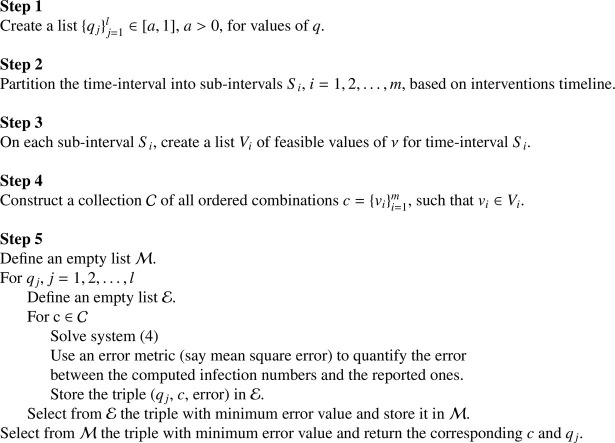
On the other hand, as outlined in Algorithm 1 , the optimal values of the fractional order $q$ and governmental intervention strength $\nu$ will be identified using the given data sets.

Table 1.

Model parameters with possible range of values together with references.

Model Parameters	Range of values	References
Baseline Transmission rate, ${\beta }_0$	0.5 - 1.5	[29]
Governmental intervention strength, $\nu$	[0,1)	[1], [21]
Intensity of behavioral response, $\kappa$	$[0,\infty )$	[1], [21]
Mean latent period, ${\sigma }^{-1}$	2 - 14 days	[30]
Mean infectious period, ${\gamma }^{-1}$	5 days	[1]
Proportion of severe cases, $\varphi$	0.2	[1]
Mean duration of public reaction, ${\omega }^{-1}$	11.2 days	[1], [21]

Algorithm 1.

Approximating the optimal $q\text{and}\nu$ pair

Based on the timeline of governmental interventions, the numerical values assumed by the parameter $\nu$ may vary on different time intervals. For the implementation of Algorithm 1, feasible values of this parameter should reflect the intensity of the interventions. For example, periods with strict regulations should have no smaller values of $\nu$ than those with relaxed interventions. As such, at the initial phase of the pandemic and before any governmental intervention, we set $\nu$ to 0. On the other hand, based on the studies in [29], [31], substantial values of $\nu$ can be considered when accounting for the effect of mandatory use of face mask and physical distancing in public places.

The intensity $\kappa$ was estimated in the study of Influenza pandemic by He et al. [21] as $\kappa =1117.3$. However, by studying and matching different data sets of COVID-19 infections, we observed that to better reflect the human behavioral response, piecewise adjustments to this value are to be considered to reflect the interventions timeline. In particular, we use $\kappa =0$ at the early stage of the outbreak since it is assumed that adequate awareness and precautions are not yet in place. For approximating $q$ and $\nu$ in Algorithm 1, we use the value $\kappa =1117.3$ for later time intervals. Nonetheless, when most of the governmental lockdown measures are being lifted, it is noted that the intensity of human behavioral response plays a major role in the decline of the number of infections. Thus, once the optimal values of $\nu$ and $q$ are approximated, we fine-tune $\kappa$ in order to achieve better matching.

In all our case studies, we implement the GETD2 scheme with a step-size $k=0.1$. Also, the root mean square error (RMSE) is used as the error metric in the implementation of Algorithm 1.

In all our simulations, the values of the RMSE between the approximated infected population and the actual data is provided for optimal $q$ and $q=1$. Moreover, to give a perspective of the corresponding relative error, we also present the values of the mean absolute percentage error (MAPE).

5.1. Case study: outbreak in Mainland China

In Table 2 , we consider the reported data of cumulative COVID-19 infections in Mainland China from January 19, 2020 to March 6, 2020, as provided in [32]. To simulate the outbreak of the pandemic, we use the

$${\beta }_0=0.52,\mu =1/(76.91\times 365),$$

together with those given in (7). Furthermore, the initial populations are

$$N_0=14000000,E_0=1000,I_0=93,R_0=0,P_0=0.$$

Table 2.

Cumulative data of number of infections in Mainland China between January 19, 2020 and March 6, 2020 as reported in [32].

January
19	20	21	22	23	24	25	26	27	28
198	291	440	571	830	1287	1975	2744	4515	5974
29	30	31
7711	9692	11791
February
1	2	3	4	5	6	7	8	9	10
14380	17205	20438	24324	28018	31161	34546	37198	40171	42638
11	12	13	14	15	16	17	18	19	20
44653	46472	48467	49970	51091	53139	55027	56776	57593	58482
21	22	23	24	25	26	27	28	29
58879	59527	59741	60249	60655	61088	61415	61842	62415
March
1	2	3	4	5	6
62617	62742	62861	63000	63143	63242

As per the lockdown records of Chinese Administrative Division, we consider the governmental intervention in two phases. The First phase corresponds to the period Jan 20 – Feb 02 and the second one to the period Feb 03 – March 06.

Applying Algorithm 1, we obtain $q=0.93$ as an approximation of the optimal fractional order. The corresponding values of governmental intervention strength $\nu$ are given in Table 3 . For comparison purposes, we also provide the optimal values of $\nu$ for the integer order problem, $q=1$. Furthermore, the values of RMSE and MAPE in approximating the infected population are also appended.

Table 3.

Midland China, the piecewise values of $\nu$ and $\kappa$ for $q=1$ and $q=0.93,$ together with the error metrics in approximating the infected population.

Period	$\nu$ for $q=1$	$\nu$ for $q=0.93$	$\kappa$
Jan 20 – Feb 02	0	0	0
Feb 03 – Mar 06	0.945	0.875	1117.3
$q$	RMSE	MAPE
0.93	281.1	51.735
1	399.616	37.589

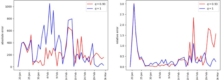
The error metrics in Table 3 suggest that the fractional order model performs better in terms of the RMSE. However, the MAPE seems to support the integer order model. This blended outcome can be understood in view of Fig. 2 . As can be observed, the absolute errors for the fractional order model are smaller throughout most of the period and thus smaller RMSE. On the other hand, although the relative errors are smaller in general for the fractional model, they attained some large values towards the end of the period, which in turn impacted the MAPE.

Fig. 2.

Mainland China, error in matching the daily reported infections. Absolute error (left), relative error (right).

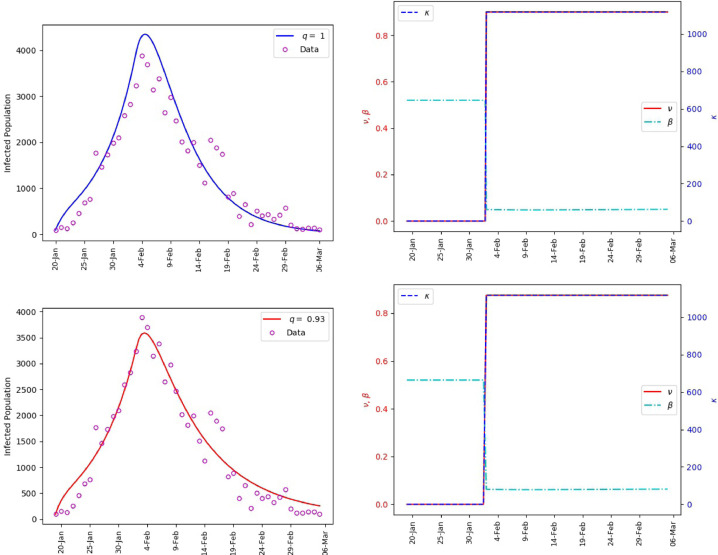
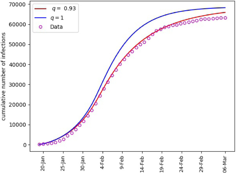
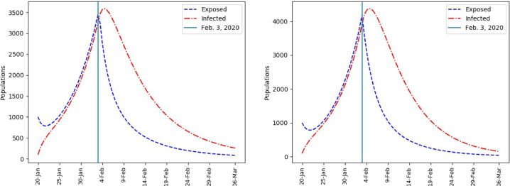
Figs. 3 and 4 include the outcomes of our simulations for the infection population and the parameters $\nu ,$ $\kappa$ and $\beta$. Fig. 5 provides an insight on the effect of governmental interventions. As observed, the change in governmental intervention strength $\nu$ on Feb 3rd yields an instantaneous change in the rate of change of exposed population. This phenomenon is expected, because governmental interventions such as inter-city lockdown, curfew, school closure among others, are expected to mitigate the contacts between susceptible and infectious individuals. However, some increase in the number of infections is still observed. This accounts for the individuals who were incubating the virus before implementation of the governmental interventions.

Fig. 3.

Mainland China, matching of the reported daily infections (left). The values of $\nu ,$$\kappa$ and the corresponding transmission rate $\beta$ (right).

Fig. 4.

Mainland China, matching of cumulative number of infections.

Fig. 5.

Mainland China, Infected and Exposed population. $q$ = 0.93 (left), $q$ = 1 (right).

Our numerical experiments also demonstrate the robustness of the fractional-order model as a generalization of the integer-order model. It is observed that the fractional order model gives extra degree of freedom, via the order of differentiation $q,$ for data fitting.

5.2. Case study: outbreak in Saudi Arabia

Since the outbreak of COVID-19 in Saudi Arabia, the Kingdom has witnessed several phases of governmental interventions aimed at mitigating spread of the diseases. Due to seasonality, special breaks and festivals, there have been a number of relaxations and tightening of these interventions.

To simulate the outbreak of the Pandemic within the Kingdom, we only adopt those interventions that were implemented at a national scale, as provided in https://www.garda.com/crisis24/news-alerts/334921/saudi-arabia-curfew-hours-modified-for-ramadan-april-21-update-29. We consider the parameters in (7) together with

$${\beta }_0=0.54,\mu =1/(75.13\times 365).$$

The initial conditions are

$$N_0=34813867,E_0=50,I_0=1,R_0=0,P_0=0.$$

Based on the data provided in https://ourworldindata.org/coronavirus-source-data, our simulation is performed for the period of March 03 to July 17 excluding the days 4th, 5th and 7th of March, where there was no reported data.

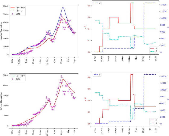
Using Algorithm 1, we obtained an approximation of the optimal $q\text{and}\nu$ pair, with $q=0.87$. For comparison purposes, we present in Table 4 the $\nu$ values corresponding to both $q=0.87$ and $q=1$. In addition, the values of the RMSE and MAPE in approximating the infected population for these values of $q$ are presented. Brief remarks on the governmental actions and the values of intensity $\kappa$ are also provided.

Table 4.

Saudi Arabia, timelines of nationwide governmental interventions and the corresponding approximated values of $\nu$ and $\kappa ,$ together with the RMSE and MAPE in approximating the infected population.

Date	Remark	$\nu$ for $q=1$	$\nu$ for $q=0.87$	$\kappa$
03-Mar	Discovery of the first cases in KSA	0	0	0
16-Mar	Closure of schools	0.1	0.1	0
23-Mar	Implementation of nationwide 7pm–6am curfew	0.4	0.25	111.73
06-Apr	Nationwide 3pm - 6am curfew and suspension of intercity travels	0.6	0.425	558.65
26-Apr	Relaxation of Nation curfew (5pm–9am) and intercity travels during Ramadan	0.5	0.4	558.65
23-May	Implementation of nationwide 24 h curfew	0.8478	0.8478	1117.3
28-May	Curfew 3pm–6am	0.45	0.5	1117.3
31-May	Relaxation of curfew (8pm–6am) and inter-region travels	0.4	0.3	4469.2
21-Jun	Return to normalcy with mandatory face masking and physical distancing measures	0.4	0.3	14524.9
$q$	RMSE	MAPE
0.87	425.917	7.907
1	603.735	10.632

We observe that the values of $\nu$ presented in Table 4 reflect the intensity of the control measures in the sense that periods with more restrictive interventions have higher values of $\nu$. From an epidemiology perspective, these interventions such as imposing a curfew, restricting the gatherings size, among others, reduce interactions and consequently mitigate the spread of the disease. As a result, the fitted values of $\nu$ tend to reflect the epidemiological reality since bigger values of $\nu$ will imply smaller values of the transmission rate $\beta$ in (2).

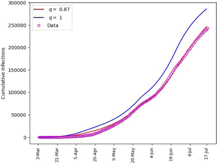
Fig. 6 includes plots of the daily infections obtained from the fractional model (1) and plots of the parameters $\nu ,$ $\kappa$ and $\beta$. It is observed that the polynomial behavior of the data at the early stage of the outbreak is better captured by the power-law corresponding to $q=0.87$ than by the exponential or almost exponential law, $q=1$ or $q=0.98$. However, the final stage of simulation is better captured with $q=0.98$. This Further illustrates the effectiveness of fractional order models for making predictions. The outcome of our simulation for the cumulative infections is presented in Fig. 7 . We note that $q=0.87$ yields a satisfactory matching.

Fig. 6.

Saudi Arabia, matching of the reported daily infections (left). The values of $\nu ,$$\kappa$ and the corresponding transmission rate $\beta$ (right).

Fig. 7.

Saudi Arabia, matching of cumulative number of infections.

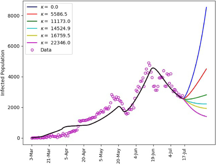
Using the calibrated model (1), predictions for the spread of the disease subject to different values of $\kappa$ are shown in Fig. 8 . We assume that the governmental intervention continues to be the same as recent period. It is shown that, a drop in the intensity $\kappa$ below the value between 21-June and 17-July will yield a spike in the infection numbers. On the other hand, maintaining same intensity will help obtain a slow decline of the infection numbers. However, a notable decay in the number of infections could be achieved if there is a significant increase in the intensity of the behavioral response. This corresponds to improved compliance with proper hand-washing, face masking, physical distancing, among others.

Fig. 8.

Saudi Arabia, matching of reported daily infections up to July 17 with $q=0.98,$ and predictions subject to different human behavioral response $\kappa$ for the period July 18–August 7.

5.3. Case study: outbreak in Italy

In the early outbreak of COVID-19 in Italy, the country was hit badly and a number of governmental interventions were initiated. To simulate this outbreak using (1), we consider

$${\beta }_0=0.75,\mu =1/(83.51\times 365),$$

together with those provided in (7). The initial conditions are

$$N_0=60461828,E_0=150,I_0=3,R_0=0,P_0=0.$$

The timeline of governmental interventions considered for this simulation are based on the report by Briscese et al. [33], up to 3-April, together with other reopening information available on https://www.bbc.com/news/world-europe-52435273. Our simulation covers the period of 31-January 2020 to 17-July 2020, based on the data provided in https://ourworldindata.org/coronavirus-source-data. However for the period February 01-21, 2020, no new infections were reported. Consequently, we excluded these dates from our simulation.

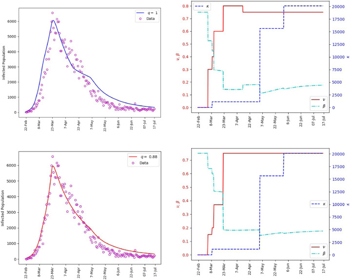
Algorithm 1 applied to the fractional order model (1) yields an approximation for the optimal $q$ and $\nu$ pair, with $q=0.88$. The corresponding values of $\nu$ are provided in Table 5 . In addition, brief descriptions of the governmental actions together with the adopted values of $\kappa$ are also provided. Similar to Saudi Arabia case, we observe that the fitted values of $\nu$ reflect the intensity of governmental actions and are consistent from an epidemiological point of view.

Table 5.

Italy, timelines of nationwide governmental interventions and the corresponding approximated values of $\nu$ and $\kappa ,$ together with the RMSE and MAPE in approximating the infected population.

Date	Remarks	$\nu$ for $q=1$	$\nu$ for $q=0.88$	$\kappa$
22-Feb		0	0	0
4-Mar	Closure of Schools	0.3	0.15	0
9-Mar	Lockdown Measures	0.4	0.2	111.73
11-Mar	Closure ofmost retail stores	0.6	0.375	558.65
22-Mar	Suspension of all non-essential economic activities	0.8	0.75	558.65
14-Apr	Re-opening of some retail activities	0.75	0.75	11173
4-May	Re-opening of salon, museums, bars among others	0.75	0.75	15642.2
1-Jun	Re-opening of more economic and sporting activities	0.75	0.75	20111.4
$q$	RMSE	MAPE
0.88	425.917	7.907
1	547.329	8.740

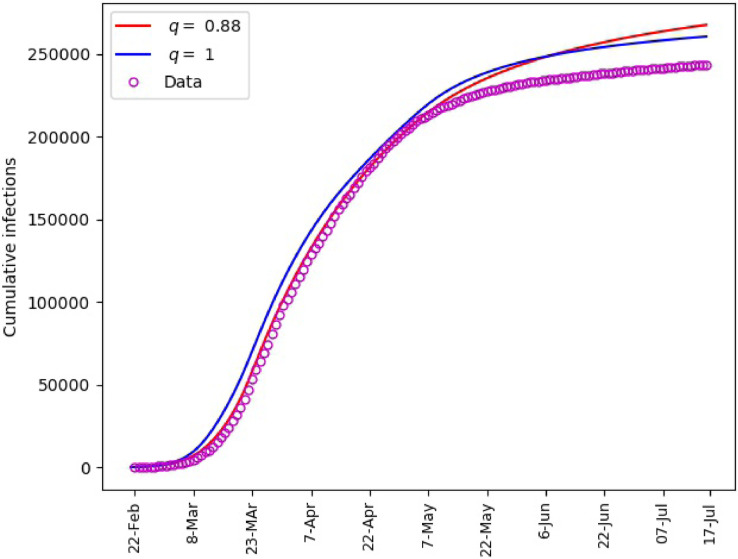
Plots of the daily and cumulative infections obtained from the model (1) are presented in Figs. 9 and 10 , respectively. We observe from these plots that the fractional order model has a better matching. This observation is also supported by the values of the error metrics included in Table 5.

Fig. 9.

Italy, matching of the reported daily infections (left). The values of $\nu ,$$\kappa$ and the corresponding transmission rate $\beta$ (right).

Fig. 10.

Italy, matching of cumulative number of infections.

5.4. Case study: outbreak in Brazil

Information from various sources indicate that there were no governmental control measures to mitigate the COVID-19 outbreak in Brazil. Some of the events in the early days of the outbreak can be found in an article by Reuters https://www.reuters.com/article/us-health-coronavirus-brazil-timeline/timeline-key-moments-in-bolsonaros-handling-of-covid-19-crisis-idINKBN2482UL. Thus, for simulating the outbreak we set $\nu =0$. The simulation covers the period from 26th February to 17th July using the data provided in https://ourworldindata.org/coronavirus-source-data. We exclude the days February 27–29 and March 02–04, 08 and 10, since no infections were reported. The other parameters used in simulating (1) for the outbreak in Brazil are

$${\beta }_0=0.75,\mu =1/(75.88\times 365),$$

together with those provided in (7). The initial conditions are

$$N_0=212,559,409,E_0=10,I_0=1,R_0=0,P_0=0.$$

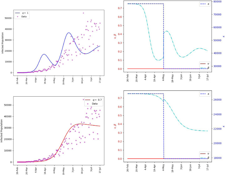
With $\nu =0$ for the whole simulation time, implementation of Algorithm 1reduces to approximating only the optimal fractional order $q,$ which is approximated as $q=0.70$.

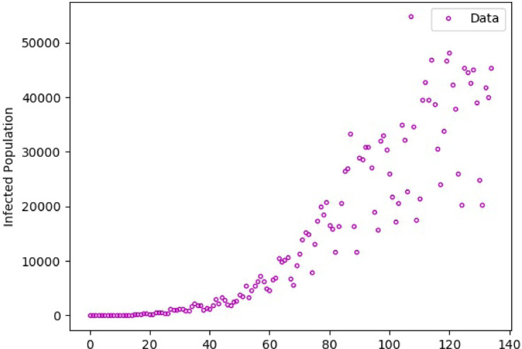
Our examination of the infection data in Fig. 11 shows that there is a significant change in the reported numbers around day sixty. Under no governmental interventions, the parameter in our model that can be used to account for this dramatic change is the human behavioral response $\kappa$. For this purpose, we split our time interval into [0, 60] and [61, 134]. Then, we fit appropriate values of $\kappa$ for both $q=0.70$ (the optimal value of $q$) and $q=1$. The calculated values are shown in Table 6 together with the RMSE and MAPE in approximating the daily number of infections.

Fig. 11.

Reported daily infections in Brazil.

Table 6.

Brazil, the piecewise values of $\kappa$ for $q=1$ and $q=0.70,$ together with the RMSE and MAPE in approximating the infected population.

Period	$\kappa$ for $q=1$	$\kappa$ for $q=0.70$
Feb 26 – May 04	80445.6	26815.2
May 05 – July 17	27932.5	17876.8
$q$	RMSE	MAPE
0.70	6732.751	48.414
1	11783.101	145.99

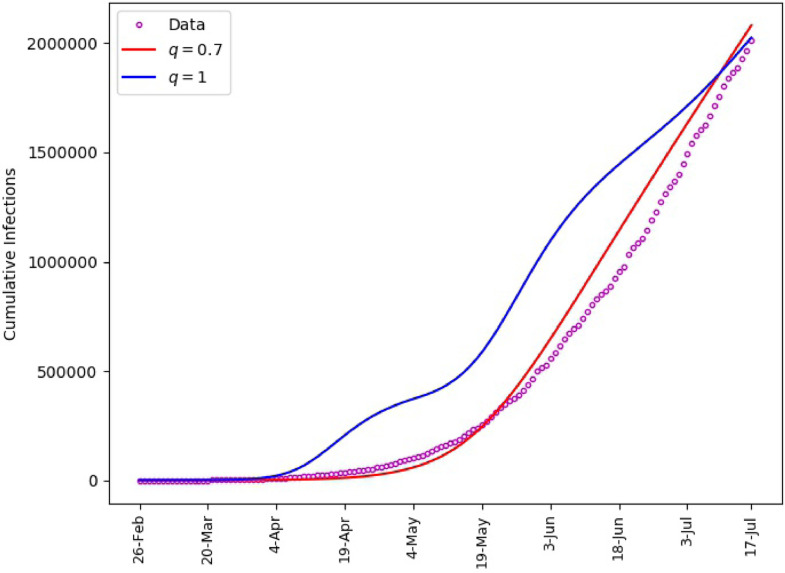
Plots of the daily infections obtained from (1) are presented in Fig. 12 . As can be observed, the integer order model could not provide a reasonable matching of the data. On the other hand, the fractional order model with $q=0.70$ is able to capture well the initial spread of the disease. Plots of the cumulative infections are also presented in 13 .

Fig. 12.

Brazil, matching of the reported daily infections in (left). The values of $\nu ,$$\kappa$ and the corresponding transmission rate $\beta$ (right).

Fig. 13.

Brazil, Matching of cumulative number of infections.

Overall, we remark that modeling the COVID-19 outbreak in Brazil is not a trivial task due to the erratic nature of the reported data. However, using the extra degree of freedom offered by the fractional order model through the fractional order $q,$ we are able to find a possible fit for daily infection data.

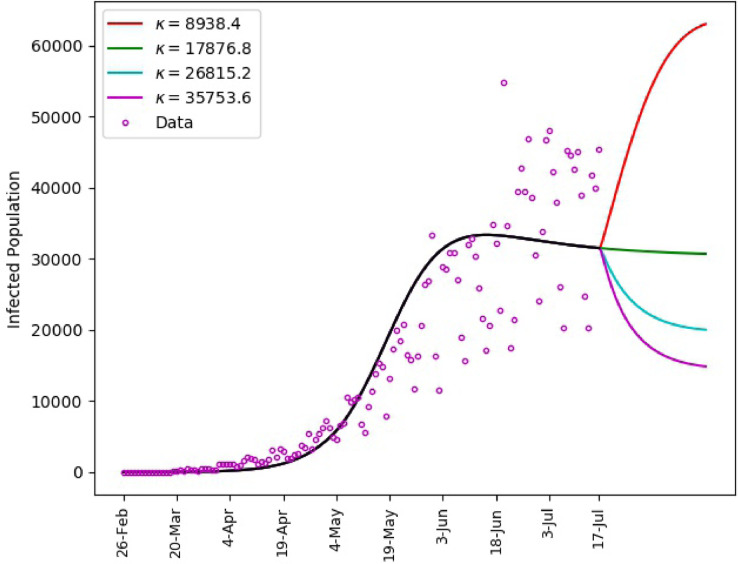
Using the calibrated model (1), predictions for the spread of the disease subject to different values of $\kappa$ are shown in Fig. 14 . For the period from February 26 to July 17, we use the values given in Table 6 for $q=0.70$. Then we predict possible infection numbers for the period from July 18 to August 16. The plots suggest that for a significant reduction in infections, a substantial increase in $\kappa$ is required. This corresponds to improved compliance with proper hand-washing, face masking, physical distancing, among other public health measures.

Fig. 14.

Brazil, matching of reported daily infections up to 17-July with $q=0.7,$ and predictions subject different human behavioral response $\kappa ,$ from 18-July to 16-August.

6. Discussion

The proposed model aims for improved fitting of the real data and thus more realistic predictions. It provides extra degrees of freedom through the fractional order $q$ and the transmission rate $\beta \left(t\right)$ that includes the government intervention and intensity of human behavioral response.

From the outcomes of our numerical simulations, we note the following observations which can help in policy making for public health interventions.

• •The data matching reveals that strict governmental lockdown measures result in large values of the parameter $\nu ,$ and thus rapid decrease in the transmission rate. This is notably observed in the case of China.
• •The intensity of human behavioral response, such as adherence to masking, hand washing, physical distancing, among others, compliments the governmental interventions in mitigating the transmission of the disease. This is demonstrated by the predictions in Fig. 8, where we see that for fixed governmental interventions, the number of infections is inversely proportional to the behavioral response $\kappa$.
• •Complete absence of governmental interventions results in growing transmission of the disease even with strong human behavioral response. This scenario is demonstrated in the Brazil model, where we set $\nu$ to zero since there is no record of governmental interventions. As can be observed, the human behavioral response alone is not adequate to mitigate the spread of the disease. Rather, it complements the governmental interventions.
• •As a consequence of the above observations, gradual lifting of governmental measures is advisable. For example, interventions such as mandatory physical distancing and masking in public places should be in place. These less strict interventions can still be well complemented by the behavioral responses and consequently help flatten the curve. The prediction for Saudi Arabia in Fig. 8 is a typical reference.

Conclusion

In this paper, we proposed a nonlinear fractional order model to study the dynamics of COVID-19 pandemic. Using the data of the outbreak in Mainland China, Saudi Arabia, Italy, and Brazil, the effectiveness of the proposed model in simulating the spread of the disease is demonstrated. Predictions based on varying intensity of human behavioral responses are provided. By examining the mean square error of the predicted number of infections and the reported data, we found that the proposed fractional model yields better matching than the integer order model. From the perspective of relative error, the values of mean absolute percentage error confirm this conclusion for the simulation of outbreak in Saudi Arabia, Italy and Brazil. On the other hand, for China, these two error metrics have mixed outcomes.

References

- 1.Lin Q., Zhao S., Gao D., Lou Y., Yang S., Musa S.S., Wang M.H., Cai Y., Wang W., Yang L., He D. A conceptual model for the coronavirus disease 2019 (COVID-19) outbreak in Wuhan, China with individual reaction and governmental action. Int. J. Infect. Dis. 2020;93:211–216. doi: 10.1016/j.ijid.2020.02.058. [DOI] [PMC free article] [PubMed] [Google Scholar]
- 2.Liu Y., Gayle A.A., Wilder-Smith A., Rocklöv J. The reproductive number of COVID-19 is higher compared to SARS coronavirus. J. Travel Med. 2020:1–4. doi: 10.1093/jtm/taaa021. [DOI] [PMC free article] [PubMed] [Google Scholar]
- 3.Diethelm K. A fractional calculus based model for the simulation of an outbreak of dengue fever. Nonlinear Dyn. 2012;71(4):613–619. [Google Scholar]
- 4.Sardar T., Rana S., Bhattacharya S., Al-Khaled K., Chattopadhyay J. A generic model for a single strain mosquito-transmitted disease with memory on the host and the vector. Math. Biosci. 2015;263:18–36. doi: 10.1016/j.mbs.2015.01.009. [DOI] [PubMed] [Google Scholar]
- 5.Hamdan N., Kilicman A. A fractional order SIR epidemic model for dengue transmission. Chaos Solitons Fractals. 2018;114:55–62. [Google Scholar]
- 6.González-Parra G., Arenas A.J., Chen-Charpentier B.M. A fractional order epidemic model for the simulation of outbreaks of influenza A (H1N1) Math. Methods Appl. Sci. 2014;37(15):2218–2226. [Google Scholar]
- 7.Ullah S., Khan M.A., Farooq M. A fractional model for the dynamics of TB virus. Chaos Solitons Fractals. 2018;116:63–71. [Google Scholar]
- 8.Jajarmi A., Baleanu D. A new fractional analysis on the interaction of HIV with CD4 T-cells. Chaos Solitons Fractals. 2018;113:221–229. [Google Scholar]
- 9.Iqbal Z., Ahmed N., Baleanu D., Adel W., Rafiq M., Aziz-ur Rehman M., Alshomrani A.S. Positivity and boundedness preserving numerical algorithm for the solution of fractional nonlinear epidemic model of HIV/AIDS transmission. Chaos Solitons Fractals. 2020;134:109706. [Google Scholar]
- 10.Pinto C.M.A., Machado J.A.T. Fractional model for malaria transmission under control strategies. Comput. Math. Appl. 2013;66:908–916. [Google Scholar]
- 11.Z. Lu, Y. Yu, Y. Chen, G. Ren, C. Xu, S. Wang, Z. Yin, A fractional-order SEIHDR model for COVID-19 with inter-city networked coupling effects, arXiv:2004.12308 (2020). [DOI] [PMC free article] [PubMed]
- 12.Bahloul M.A., Chahid A., Laleg-Kirati T.-M. Fractional-order SEIQRDP model for simulating the dynamics of COVID-19 epidemic. IEEE Open J. Eng. Med. Biol. 2020;1:249–256. doi: 10.1109/OJEMB.2020.3019758. [DOI] [PMC free article] [PubMed] [Google Scholar]
- 13.Higazy M. Novel fractional order SIDARTHE mathematical model of COVID-19 pandemic. Chaos Solitons Fractals. 2020;138:110007. doi: 10.1016/j.chaos.2020.110007. [DOI] [PMC free article] [PubMed] [Google Scholar]
- 14.Zhang Y., Yu X., Sun H., Tick G.R., Wei W., Jin B. Applicability of time fractional derivative models for simulating the dynamics and mitigation scenarios of COVID-19. Chaos Solitons Fractals. 2020;138:109959. doi: 10.1016/j.chaos.2020.109959. [DOI] [PMC free article] [PubMed] [Google Scholar]
- 15.Podlubny I. Geometric and physical interpretation of fractional integration and fractional differentiation. Fract. Calc. Appl. Anal. 2002;5(4):367–386. [Google Scholar]
- 16.Popović J.K., Atanacković M.T., Pilipović A.S., Rapaić M.R., Pilipović S., Atanacković T.M. A new approach to the compartmental analysis in pharmacokinetics: fractional time evolution of diclofenac. J. Pharmacokinet. Pharmacodyn. 2010;37:119–134. doi: 10.1007/s10928-009-9147-3. [DOI] [PubMed] [Google Scholar]
- 17.Dokoumetzidis A., Magin R., Macheras P. Fractional kinetics in multi-compartmental systems. J. Pharmacokinet. Pharmacodyn. 2010;37:507–524. doi: 10.1007/s10928-010-9170-4. [DOI] [PubMed] [Google Scholar]
- 18.Angstmann C.N., Henry B.I., McGann A.V. A fractional-order infectivity SIR model. Phys. A Stat. Mech. Appl. 2016;452:86–93. [Google Scholar]
- 19.Islam M.R., Peace A., Medina D., Oraby T. Integer versus fractional order SEIR deterministic and stochastic models of Measles. Int. J. Environ. Res. Public Health. 2020;17(6):2014. doi: 10.3390/ijerph17062014. [DOI] [PMC free article] [PubMed] [Google Scholar]
- 20.Tuan N.H., Mohammadi H., Rezapour S. A mathematical model for COVID-19 transmission by using the Caputo fractional derivative. Chaos Solitons Fractals. 2020;140:110107. doi: 10.1016/j.chaos.2020.110107. [DOI] [PMC free article] [PubMed] [Google Scholar]
- 21.He D., Dushoff J., Day T., Ma J., Earn D.J. Inferring the causes of the three waves of the 1918 influenza pandemic in England and Wales. Proc. R. Soc. B Biol. Sci. 2013;280:20131345. doi: 10.1098/rspb.2013.1345. [DOI] [PMC free article] [PubMed] [Google Scholar]
- 22.Garappa R., Popolizio M. Generalized exponential time differencing methods for fractional order problems. Comput. Math. Appl. 2011;62:876–890. [Google Scholar]
- 23.Sarumi I.O., Furati K.M., Khaliq A.Q.M. Highly accurate global PadȨ approximations of generalized MittagLeffler function and its inverse. J. Sci. Comput. 2020;82(46) [Google Scholar]
- 24.Li Y., Chen Y., Podlubny I. MittagLeffler stability of fractional order nonlinear dynamic systems. Automatica. 2009;45(8):1965–1969. [Google Scholar]
- 25.Diekmann O., Heesterbeek J.A.P., Metz J.A.J. On the definition and the computation of the basic reproduction ratio in models for infectious diseases in heterogeneous populations. J. Math. Biol. 1990;28(4):365–382. doi: 10.1007/BF00178324. [DOI] [PubMed] [Google Scholar]
- 26.van den Driessche P., Watmough J. Reproduction numbers and sub-threshold endemic equilibria for compartmental models of disease transmission. Math. Biosci. 2002;180(1):29–48. doi: 10.1016/s0025-5564(02)00108-6. [DOI] [PubMed] [Google Scholar]
- 27.Ahmed E., El-Sayed A.M.A., El-Saka H.A.A. Equilibrium points, stability and numerical solutions of fractional-order predatorprey and rabies models. J. Math. Anal. Appl. 2007;325(1):542–553. [Google Scholar]
- 28.Matignon D. Computational Engineering in Systems Applications. 1996. Stability results for fractional differential equations with applications to control processing; pp. 963–968. [Google Scholar]
- 29.Eikenberry S.E., Mancuso M., Iboi E., Phan T., Eikenberry K., Kuang Y., Kostelich E., Gumel A.B. To mask or not to mask: modeling the potential for face mask use by the general public to curtail the COVID-19 pandemic. Infect. Dis. Model. 2020;5:293–308. doi: 10.1016/j.idm.2020.04.001. [DOI] [PMC free article] [PubMed] [Google Scholar]
- 30.Guan W.-j., Ni Z.-y., Hu Y., Liang W.-h., Ou C.-q., He J.-x., Liu L., Shan H., Lei C.-l., Hui D.S., et al. Clinical characteristics of 2019 novel coronavirus infection in China. MedRxiv. 2020 [Google Scholar]
- 31.Sande M., Teunis P., Sabel R. Professional and home-made face masks reduce exposure to respiratory infections among the general population. PloS One. 2008;3(7):e2618. doi: 10.1371/journal.pone.0002618. [DOI] [PMC free article] [PubMed] [Google Scholar]
- 32.Z. Liu, P. Magal, O. Seydi, G. Webb, Predicting the cumulative number of cases for the COVID-19 epidemic in China from early data, arXiv:2002.12298 (2020). [DOI] [PubMed]
- 33.Briscese G., Lacetera N., Macis M., Tonin M. Technical Report. National Bureau of Economic Research; 2020. Compliance with Covid-19 social-distancing measures in Italy: the role of expectations and duration. [Google Scholar]