

Abstract
Semi-competing risks refer to the setting where primary scientific interest lies in estimation and inference with respect to a non-terminal event, the occurrence of which is subject to a terminal event. In this paper, we present the R package SemiCompRisks that provides functions to perform the analysis of independent/clustered semi-competing risks data under the illness-death multi-state model. The package allows the user to choose the specification for model components from a range of options giving users substantial flexibility, including: accelerated failure time or proportional hazards regression models; parametric or non-parametric specifications for baseline survival functions; parametric or non-parametric specifications for random effects distributions when the data are cluster-correlated; and, a Markov or semi-Markov specification for terminal event following non-terminal event. While estimation is mainly performed within the Bayesian paradigm, the package also provides the maximum likelihood estimation for select parametric models. The package also includes functions for univariate survival analysis as complementary analysis tools.
Introduction
Semi-competing risks refer to the general setting where primary scientific interest lies in estimation and inference with respect to a non-terminal event (e.g., disease diagnosis), the occurrence of which is subject to a terminal event (e.g., death) (Fine et al., 2001; Jazić et al., 2016). When there is a strong association between two event times, naïive application of a univariate survival model for non-terminal event time will result in overestimation of outcome rates as the analysis treats the terminal event as an independent censoring mechanism (Haneuse and Lee, 2016). The semi-competing risks analysis framework appropriately treats the terminal event as a competing event and considers the dependence between non-terminal and terminal events as part of the model specification.
Toward formally describing the structure of semi-competing risks data, let T1 and T2 denote the times to the non-terminal and terminal events, respectively. From the modeling perspective, the focus in the semi-competing risks setting is to characterize the distribution T1 and its potential relationship with the distribution of T2, i.e. the joint distribution of (T1, T2). For example, from an initial state (e.g., transplantation), as time progresses, a subject could make a transition into the non-terminal or terminal state (see Figure 1.a). In the case of a transition into the non-terminal state, the subject could subsequently transition into the terminal state even if these transitions cannot occur in the reverse order. The main disadvantage of the competing risks framework (see Figure 1.b) to the study of non-terminal event is that it does not utilize the information on the occurrence and timing of terminal event following the non-terminal event, which could be used to understand the dependence between the two events.
Figure 1:
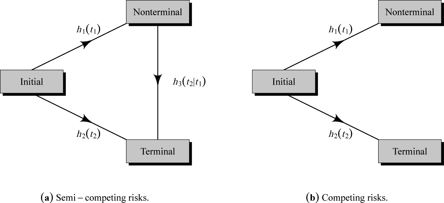
Graphical representation of (a) semi-competing risks and (b) competing risks.
The current literature for the analysis of semi-competing risks data is composed of three approaches: methods that specify the dependence between non-terminal and terminal events via a copula (Fine et al., 2001; Wang, 2003; Jiang et al., 2005; Ghosh, 2006; Peng and Fine, 2007; Lakhal et al., 2008; Hsieh et al., 2008; Fu et al., 2013); methods based on multi-state models, specifically the so-called illness-death model (Liu et al., 2004; Putter et al., 2007; Ye et al., 2007; Kneib and Hennerfeind, 2008; Zeng and Lin, 2009; Xu et al., 2010; Zeng et al., 2012; Han et al., 2014; Zhang et al., 2014; Lee et al., 2015, 2016); and methods built upon the principles of causal inference (Zhang and Rubin, 2003; Egleston et al., 2007; Tchetgen Tchetgen, 2014; Varadhan et al., 2014).
The SemiCompRisks package is designed to provide a comprehensive suite of functions for the analysis of semi-competing risks data based on the illness-death model, together with, as a complementary suite of tools, functions for the analysis of univariate time-to-event data. While Bayesian methods are used for estimation and inference for all available models, maximum likelihood estimation is also provided for select parametric models. Furthermore, SemiCompRisks offers flexible parametric and non-parametric specifications for baseline survival functions and cluster-specific random effects distributions under accelerated failure time and proportional hazards models. The functionality of the package covers methods proposed in a series of recent papers on the analysis of semi-competing risks data (Lee et al., 2015, 2016, 2017c).
The remainder of the paper is organized as follows. Section Other packages and their features summarizes existing R packages that provide methods for multi-state modeling, and explains the key contributions of the SemiCompRisks package. Section CIBMTR data introduces an on-going study of stem cell transplantation and provides a description of the data available in the package. Section The illness-death models for semi-competing risks data presents different specifications of models and estimation methods implemented in our package. Section Package description summarizes the core components of the SemiCompRisks package, including datasets, functions for fitting models, functions, the structure of output provided to analysts. Section Illustration: Stem cell transplantation data illustrates the usage of the main functions in the package through three semi-competing risks analyses of the stem cell transplantation data. Finally, Section Discussion concludes with discussion and an overview of the extensions we are working on.
Other packages and their features
As we elaborate upon below, the illness-death model for semi-competing risks, that is the focus on the SemiCompRisks package, is a special case of the broader class of multi-state models. Currently, there are numerous R packages that permit estimation and inference for a multi-state model and that could conceivably be used to analyze semi-competing risks data.
The mvna package computes the Nelson-Aalen estimator of the cumulative transition hazard for arbitrary Markov multi-state models with right-censored and left-truncated data, but it does not compute transition probability matrices (Allignol et al., 2008). The TPmsm implements non-parametric and semi-parametric estimators for the transition probabilities in 3-state models, including the Aalen-Johansen estimator and estimators that are consistent even without Markov assumption or in case of dependent censoring (Araújo et al., 2014). The p3state.msm package performs inference in an illness-death model (Meira-Machado and Roca-Pardiñas, 2011). Its main feature is the ability for obtaining non-Markov estimates for the transition probabilities. The etm package calculates the empirical transition probability matrices and corresponding variance estimates for any time-inhomogeneous multi-state model with finite state space and data subject to right-censoring and left-truncation, but it does not account for the influence of covariates (Allignol et al., 2011). The msm package is able to fit time-homogeneous Markov models to panel count data and hidden Markov models in continuous time (Jackson, 2011). The time-homogeneous Markov approach could be a particular case of the illness-death model, where interval-censored data can be considered. The tdc.msm package may be used to fit the time-dependent proportional hazards model and multi-state regression models in continuous time, such as Cox Markov model, Cox semi-Markov model, homogeneous Markov model, non-homogeneous piecewise model, and non-parametric Markov model (Meira-Machado et al., 2007). The SemiMarkov package performs parametric (Weibull or exponentiated Weibull specification) estimation in a homogeneous semi-Markov model (Król and Saint-Pierre, 2015). Moreover, the effects of covariates on the process evolution can be studied using a semi-parametric Cox model for the distributions of sojourn times. The flexsurv package provides functions for fitting and predicting from fully-parametric multi-state models with Markov or semi-Markov specification (Jackson, 2016). In addition, the multi-state models implemented in flexsurv give the possibility to include interval-censoring and some of them also left-truncation. The msSurv calculates non-parametric estimation of general multi-state models subject to independent right-censoring and possibly left-truncation (Ferguson et al., 2012). This package also computes the marginal state occupation probabilities along with the corresponding variance estimates, and lower and upper confidence intervals. The mstate package can be applied to right-censored and left-truncated data in semi-parametric or non-parametric multi-state models with or without covariates and it may also be used to competing risk models (Wreede et al., 2011). Specifically for Cox-type illness-death models to interval-censored data, we highlight the packages coxinterval (Boruvka and Cook, 2015) and SmoothHazard (Touraine et al., 2017), where the latter also allows that the event times to be left-truncated. Finally, frailtypack package permits the analysis of correlated data under select clusterings, as well as the analysis of left-truncated data, through a focus on frailty models using penalized likelihood estimation or parametric estimation (Rondeau et al., 2012).
While these packages collectively provide broad functionality, each of them is either non-specific to semi-competing risks or only permits consideration of a narrow model specifications. In developing the SemiCompRisks package, the goal was to provide a single package within which a broad range of models and model specifications could be entertained. The frailtypack package, for example, can also be used to analyze cluster-correlated semi-competing risks data but it is restricted to the proportional hazards model with either patient-specific or cluster-specific random effects but not both (Liquet et al., 2012). Furthermore, estimation/inference is within the frequentist framework so that estimation of hospital-specific random effects, of particular interest in health policy applications (Lee et al., 2016), together with the quantification of uncertainty is incredibly challenging. This, however, is (relatively) easily achieved through the functionality of SemiCompRisks package. Given the breadth of the functionality of the package, in addition to the usual help files, we have developed a series of model-specific vignettes which can be accessed through the CRAN (Lee et al., 2017b) or R command vignette(“SemiCompRisks”), covering a total of 12 distinct model specifications.
CIBMTR data
The example dataset used throughout this paper was obtained from the Center for International Blood and Marrow Transplant Research (CIBMTR), a collaboration between the National Marrow Donor Program and the Medical College of Wisconsin representing a worldwide network of transplant centers (Lee et al., 2017a). For illustrative purposes, we consider a hypothetical study in which the goal is to investigate risk factors for grade III or IV acute graft-versus-host disease (GVHD) among 9, 651 patients who underwent the first allogeneic hematopoietic cell transplant (HCT) between January 1999 and December 2011.
As summarized in Table 1, after administratively censoring follow-up at 365 days post-transplant, each patient can be categorized according to their observed outcome information into four groups: (i) acute GVHD and death; (ii) acute GVHD and censored for death; (iii) death without acute GVHD; and (iv) censored for both. Furthermore, for each patient, the following covariates are available:gender (Male, Female); age (<10, 10–19, 20–29, 30–39, 40–49, 50–59, 60+); disease type (AML, ALL, CML, MDS); disease stage (Early, Intermediate, Advanced); and HLA compatibility (Identical sibling, 8/8, 7/8).
Table 1:
Covariate and simulated outcome information for 9,651 patients who underwent the first HCT between 1999–2011 with administrative censoring at 365 days.
| N | % | Outcome category (%) | ||||
|---|---|---|---|---|---|---|
| Both acute GVHD & death | Acute GVHD & censored for death | Death without acute GVHD | Censored for both | |||
| Total subjects | 9,651 | 100.0 | 9.5 | 8.9 | 28.8 | 52.8 |
| Gender | ||||||
| Male | 5,366 | 55.6 | 9.7 | 9.5 | 28.1 | 52.7 |
| Female | 4,285 | 44.4 | 9.1 | 8.3 | 29.7 | 52.9 |
| Age, years | ||||||
| <10 | 653 | 6.8 | 5.0 | 11.9 | 23.4 | 59.7 |
| 10–19 | 1,162 | 12.0 | 8.0 | 11.4 | 24.0 | 56.6 |
| 20–29 | 1,572 | 16.3 | 9.7 | 9.9 | 27.4 | 53.0 |
| 30–39 | 1,581 | 16.4 | 9.8 | 10.7 | 28.5 | 51.0 |
| 40–49 | 2,095 | 21.7 | 11.0 | 9.6 | 29.7 | 49.7 |
| 50–59 | 2,008 | 20.8 | 9.8 | 5.1 | 32.3 | 52.8 |
| 60+ | 580 | 6.0 | 9.9 | 4.8 | 33.1 | 52.2 |
| Disease type | ||||||
| AML | 4,919 | 51.0 | 8.2 | 8.0 | 30.3 | 53.5 |
| ALL | 2,071 | 21.5 | 9.9 | 9.0 | 29.3 | 51.8 |
| CML | 1,525 | 15.8 | 12.1 | 11.3 | 22.2 | 54.4 |
| MDS | 1,136 | 11.8 | 11.0 | 10.0 | 30.0 | 49.0 |
| Disease status | ||||||
| Early | 4,873 | 50.5 | 8.4 | 11.0 | 23.6 | 57.0 |
| Intermediate | 2,316 | 24.0 | 9.7 | 8.5 | 30.1 | 51.7 |
| Advanced | 2,462 | 25.5 | 11.5 | 5.4 | 37.7 | 45.4 |
| HLA compatibility | ||||||
| Identical sibling | 3,941 | 40.8 | 7.4 | 8.5 | 26.3 | 57.8 |
| 8/8 | 4,100 | 42.5 | 10.5 | 9.7 | 30.3 | 49.5 |
| 7/8 | 1,610 | 16.7 | 12.2 | 8.1 | 30.9 | 48.8 |
We note that due to confidentiality considerations the original study outcomes (time1, time2, event1, event2: times and censoring indicators to the non-terminal and terminal events) are not available in SemiCompRisks package. As such we provide the five original covariates together with estimates of parameters from the analysis of CIBMTR data, so that one could simulate semi-competing risks outcomes (see the simulation procedure in Appendix Simulating outcomes using CIBMTR covariates). Based on this, the data shown in Table 1 reflects simulated outcome data using 1405 as the seed.
The illness-death models for semi-competing risks data
We offer three flexible multi-state illness-death models for the analysis of semi-competing risks data: accelerated failure time (AFT) models for independent data; proportional hazards regression (PHR) models for independent data; and PHR models for cluster-correlated data. These models accommodate parametric or non-parametric specifications for baseline survival functions as well as a Markov or semi-Markov assumptions for terminal event following non-terminal event.
AFT models for independent semi-competing risks data
In the AFT model specification, we directly model the connection between event times and covariates (Wei, 1992). For the analysis of semi-competing risks data, we consider the following AFT model specifications under the illness-death modeling framework (Lee et al., 2017c):
| (1) |
| (2) |
| (3) |
where Ti1 and Ti2 denote the times to the non-terminal and terminal events, respectively, from subject i = 1, … , n, xig is a vector of transition-specific covariates, βg is a corresponding vector of transition-specific regression parameters, and ϵig is a transition-specific random variable whose distribution determines that of the corresponding transition time, g ∈ {1,2,3}. Finally, in each of (1)–(3), γi is a study subject-specific random effect that induces positive dependence between the two event times. We assume that γi follows a Normal(0, θ) distribution and adopt a conjugate inverse Gamma distribution, denoted by IG(a(θ), b(θ)) for the variance component θ. For regression parameters βg, we adopt non-informative flat prior on the real line.
From models (1)–(3), we can adopt either a fully parametric or a semi-parametric approach depending on the specification of the distributions for ϵi1, ϵi2, ϵi3. We build a parametric modeling based on the log-Normal formulation, where ϵig follows a Normal(μg, ) distribution. We adopt non-informative flat priors on the real line for μg and independent IG(, ) for . As an alternative, a semi-parametric framework can be considered by adopting independent non-parametric Dirichlet process mixtures (DPM) of Mg Normal(μgr, ) distributions, r ∈ {1, … , Mg}, for each ϵig. Following convention in the literature, we refer to each component Normal distribution as being specific to some “class” (Neal, 2000). Since the class-specific (μgr, ) are unknown, they are assumed to be draws from a so-called the centering distribution. Specifically, we take a Normal distribution centered at μg0 with a variance for μgr and an for . Furthermore, since the “true” class membership for any given study subject is unknown, we let pgr denote the probability of belonging to the rth class for transition g and pg = (pg1, … , pgMg)⊤ the collection of such probabilities. In the absence of prior knowledge regarding the distribution of class memberships for the n subjects across the Mg classes, pg is assumed to follow a conjugate symmetric Dirichlet(τg/Mg, … , τg/Mg) distribution, where τg is referred to as the precision parameter (for more details, see Lee et al., 2017c).
Our AFT modeling framework can also handle interval-censored and/or left-truncated semi-competing risks data. Suppose that subject i was observed at follow-up times and let and Li denote the time to the end of study (or administrative right-censoring) and the time at study entry (i.e., the left-truncation time), respectively. Considering interval-censoring for both events, Ti1 and Ti2, for i = 1, … , n, satisfy cij ≤ Ti1 < cij+1 for some j and cik ≤ Ti2 < cik+1 for some k, respectively. Therefore, the observed outcome information for interval-censored and left-truncated semi-competing risks data for the subject i can be represented by {Li, cij, cij+1, cik, cik+1}.
PHR models for independent semi-competing risks data
We consider an illness-death multi-state model with proportional hazards assumptions characterized by three hazard functions (see Figure 1.a) that govern the rates at which subjects transition between the states: a cause-specific hazard for non-terminal event, h1(ti1); a cause-specific hazard for terminal event, h2(ti2); and a hazard for terminal event conditional on a time for non-terminal event, h3(ti2 | ti1). We consider the following specification for hazard functions (Xu et al., 2010; Lee et al., 2015):
| (4) |
| (5) |
| (6) |
where h0g is an unspecified baseline hazard function and βg is a vector of log-hazard ratio regression parameters associated with the covariates xig. Finally, in each of (4)–(6), γi is a study subject-specific shared frailty following a Gamma(θ−1, θ−1) distribution, parametrized so that E [γi] = 1 and V [γi] = θ. The model (6) is referred to as being Markov or semi-Markov depending on whether we assume z(ti1, ti2) = ti2 or z(ti1, ti2) = ti2 − ti1, respectively.
The Bayesian approach for models (4)–(6) requires the specification of prior distributions for unknown parameters. For the regression parameters βg, we adopt a non-informative flat prior distribution on the real line. For the variance in the subject-specific frailties, θ, we adopt a Gamma(a(θ), b(θ)) for the precision θ−1. For the parametric specification for baseline hazard functions, we consider a Weibull model: . We assign a Gamma(, ) for αg and a Gamma(, ) for κg. As an alternative, a non-parametric piecewise exponential model (PEM) is considered for baseline hazard functions based on taking each of the log-baseline hazard functions to be a flexible mixture of piecewise constant function. Let sg,max denote the largest observed event time for each transition and construct a finite partition of the time axis, . Letting denote the heights of the log-baseline hazard function on the disjoint intervals based on the time splits , we assume that λg follows a multivariate Normal distribution (MVN), , where is the overall mean, represents a common variance component for the Kg + 1 elements, and specifies the covariance structure these elements. We adopt a flat prior on the real line for and a conjugate Gamma(, ) distribution for the precision . In order to relax the assumption of fixed partition of the time scales, we adopt a Poisson() prior for the number of splits, Kg, and conditioned on the number of splits, we consider locations, sg, to be a priori distributed as the even-numbered order statistics:
| (7) |
Note that the prior distributions of Kg and sg jointly form a time-homogeneous Poisson process prior for the partition (Kg, sg). For more details, see Lee et al. (2015).
PHR models for cluster-correlated semi-competing risks data
Lee et al. (2016) proposed hierarchical models that accommodate correlation in the joint distribution of the non-terminal and terminal events across patients for the setting where patients are clustered within hospitals. The hierarchical models for cluster-correlated semi-competing risks data build upon the illness-death model given in (4)–(6). Let Tji1 and Tji2 denote the times to the non-terminal and terminal events for the ith subject in the jth cluster, respectively, for i = 1, … , nj and j = 1, … , J. The general modeling specification is given by:
| (8) |
| (9) |
| (10) |
where h0g is an unspecified baseline hazard function and βg is a vector of log-hazard ratio regression parameters associated with the covariates xjig. A study subject-specific shared frailty γji is assumed to follow a Gamma(θ−1, θ−1) distribution and Vj = (Vj1, Vj2, Vj3)⊤ is a vector of cluster-specific random effects, each specific to one of the three possible transitions.
From a Bayesian perspective for models (8)–(10), we can adopt either a parametric Weibull or non-parametric PEM specification for baseline hazard functions h0g with their respective configurations of prior distributions analogous to those outlined in Section PHR models for independent semi-competing risks data. For the parametric specification of cluster-specific random effects, we assume that Vj follows MVN3(0, ΣV) distribution. We adopt a conjugate inverse-Wishart(Ψv, ρv) prior for the variance-covariance matrix ΣV. For the non-parametric specification, we adopt a DPM of MVN distributions with a centering distribution, G0, and a precision parameter, τ. Here we take G0 to be a multivariate Normal/inverse-Wishart (NIW) distribution for which the probability density function can be expressed as the product:
| (11) |
where Ψ0 and ρ0 are the hyperparameters of fNIW(·). We assign a Gamma(aτ, bτ) prior distribution for τ. Finally, for βg and θ, we adopt the same priors as those adopted for the model in Section PHR models for independent semi-competing risks data. For more details, see Lee et al. (2016).
Estimation and inference
Bayesian estimation and inference is available for all models in the SemiCompRisks. Additionally, one may also choose to use maximum likelihood estimation for the parametric Weibull PHR model described in Section PHR models for independent semi-competing risks data.
To perform Bayesian estimation and inference, we use a random scan Gibbs sampling algorithm to generate samples from the full posterior distribution. Depending on the complexity of the model adopted, the Markov chain Monte Carlo (MCMC) scheme may also include additional strategies, such as Metropolis-Hastings and reversible jump MCMC (Metropolis-Hastings-Green) steps. Specific details of each implementation can be seen in the online supplemental materials of Lee et al. (2015, 2016, 2017c).
Package description
The SemiCompRisks package contains three key functions, FreqID_HReg, BayesID_HReg and BayesID_AFT, focused on models for semi-competing risks data as well as the analogous univariate survival models, FreqSurv_HReg, BayesSurv_HReg and BayesSurv_AFT. It also provides two auxiliary functions, initiate.startValues_HReg and initiate.startValues_AFT, that can be used to generate initial values for Bayesian estimation; simID and simSurv functions for simulating semi-competing risks and univariate survival data, respectively; five covariates and parameter estimates from CIBMTR data; and the BMT dataset referring to 137 bone marrow transplant patients.
Summary of functionality
Table 2 shows the modeling options implemented in the SemiCompRisks package for both semi-competing risks and univariate analysis. Specifically, we categorize the approaches based on the analysis type (semi-competing risks or univariate), the survival model (AFT or PHR), data type (independent or clustered), accommodation to left-truncation and/or interval-censoring in addition to right-censoring, and also statistical paradigms (frequentist or Bayesian).
Table 2:
Models implemented in the SemiCompRisks package.
| Analysis | Model | Data type | L-T and/or I-C | Statistical paradigm |
|---|---|---|---|---|
| Semi-competing risks | AFT | Independent | No | B |
| Yes | B | |||
| Clustered | No | x | ||
| Yes | x | |||
| PHR | Independent | No | B & F | |
| Yes | x | |||
| Clustered | No | B | ||
| Yes | x | |||
| Univariate | AFT | Independent | No | B |
| Yes | B | |||
| Clustered | No | x | ||
| Yes | x | |||
| PHR | Independent | No | B & F | |
| Yes | x | |||
| Clustered | No | B | ||
| Yes | x |
L-T: left-truncation; I-C: interval-censoring; B: Bayesian; F: frequentist; x: not available
The full description of functionality of the SemiCompRisks package can be accessed through the R command help(“SemiCompRisks”) or vignette(“SemiCompRisks”) which provides in detail the specification of all models implemented in the package. Below we describe the input data format and some crucial arguments for defining and fitting a model for semi-competing risks data using the SemiCompRisks package.
Model specification
From a semi-competing risks dataset, we jointly define the outcomes and covariates in a Formula object. Here we use the simCIBMTR dataset, obtained from the simulation procedure presented in Appendix Simulating outcomes using CIBMTR covariates:
R> form <- Formula(time1 + event1 | time2 + event2 ~ dTypeALL + dTypeCML + + dTypeMDS + sexP | dTypeALL + dTypeCML + dTypeMDS | dTypeALL + + dTypeCML + dTypeMDS)
The outcomes time1, time2, event1 and event2 denote the times and censoring indicators to the non-terminal and terminal events, respectively, and the covariates of each hazard function are separated by | (vertical bar).
The specification of the Formula object varies slightly if the semi-competing risks model accommodates left-truncated and/or interval-censored data (see vignette documentation Lee et al. (2017b)).
Critical arguments
Most functions for semi-competing risks analysis in the SemiCompRisks package take common arguments. These arguments and their descriptions are shown as follows:
id: a vector of cluster information for n subjects, where cluster membership corresponds to one of the positive integers 1, … , J.
model: a character vector that specifies the type of components in a model. It can have up to three elements depending on the model specification. The first element is for the assumption on h3: “semi-Markov” or “Markov”. The second element is for the specification of baseline hazard functions for PHR models - “Weibull” or “PEM” - or baseline survival distribution for AFT models - “LN” (log-Normal) or “DPM”. The third element needs to be set only for clustered semi-competing risks data and is for the specification of cluster-specific random effects distribution: “MVN” or “DPM”.
hyperParams: a list containing vectors for hyperparameter values in hierarchical models.
startValues: a list containing vectors of starting values for model parameters.
mcmcParams: a list containing variables required for MCMC sampling.
Hyperparameter values, starting values for model parameters, and MCMC arguments depend on the specified Bayesian model and the assigned prior distributions. For a list of illustrations, see vignette documentation Lee et al. (2017b).
FreqID_HReg
The function FreqID_HReg fits Weibull PHR models for independent semi-competing risks data, as in (4)–(6), based on maximum likelihood estimation. Its default structure is given by:
FreqID_HReg(Formula, data, model=“semi-Markov”, frailty=TRUE),
where Formula represents the outcomes and the linear predictors jointly, as presented in Section Summary of functionality; data is a data frame containing the variables named in Formula; model is one of the critical arguments of the SemiCompRisks package (see Section Summary of functionality), in which it specifies the type of model based on the assumption on h3(ti2 | ti1,·) in (6). Here, model can be “Markov” or “semi-Markov”. Finally, frailty is a logical value (TRUE or FALSE) to determine whether to include the subject-specific shared frailty term γ into the illness-death model.
BayesID_HReg
The function BayesID_HReg fits parametric and semi-parametric PHR models for independent or cluster-correlated semi-competing risks data, as in (4)–(6) or (8)–(10), based on Bayesian inference. Its default structure is given by:
BayesID_HReg(Formula, data, id=NULL, model=c(“semi-Markov”, “Weibull”), hyperParams, startValues, mcmcParams, path=NULL).
Formula and data are analogous to the previous case; id, model, hyperParams, startValues, and mcmcParams are all critical arguments of the SemiCompRisks package (see Section Summary of functionality), where id indicates the cluster that each subject belongs to (for independent data, id=NULL); model allows us to specify either “Markov” or “semi-Markov” assumption, whether the priors for baseline hazard functions are parametric (“Weibull”) or non-parametric (“PEM”), and whether the cluster-specific random effects distribution is parametric (“MVN”) or non-parametric (“DPM”). The third element of model is only required for models for clustered-correlated data given in (8)–(10).
The hyperParams argument defines all model hyperparameters: theta (a numeric vector for hyperparameters, a(θ) and b(θ), in the prior of subject-specific frailty variance component), WB (a list containing numeric vectors for Weibull hyperparameters (, ) and (, ) for g ∈ {1, 2, 3}: WB.ab1, WB.ab2, WB.ab3, WB.cd1, WB.cd2, WB.cd3), PEM (a list containing numeric vectors for PEM hyperparameters (, ), and for g ∈ {1, 2, 3}: PEM.ab1, PEM.ab2, PEM.ab3, PEM.alpha1, PEM.alpha2, PEM.alpha3); and for the analysis of clustered semi-competing risks data, additional components are required: MVN (a list containing numeric vectors for MVN hyperparameters Ψv and ρv: Psi_v, rho_v), DPM (a list containing numeric vectors for DPM hyperparameters Ψ0, ρ0, aτ, and bτ: Psi0, rho0, aTau, bTau).
The startValues argument specifies initial values for model parameters. This specification can be done manually or through the auxiliary function initiate.startValues_HReg. The mcmcParams argument sets the information for MCMC sampling: run (a list containing numeric values for setting for the overall run: numReps, total number of scans; thin, extent of thinning; burninPerc, the proportion of burn-in), storage (a list containing numeric values for storing posterior samples for subject- and cluster-specific random effects: nGam_save, the number of γ to be stored; storeV, a vector of three logical values to determine whether all the posterior samples of Vj, for j = 1, … , J are to be stored), tuning (a list containing numeric values relevant to tuning parameters for specific updates in Metropolis-Hastings-Green (MHG) algorithm: mhProp_theta_var, the variance of proposal density for θ; mhProp_Vg_var, the variance of proposal density for Vj in DPM models; mhProp_alphag_var, the variance of proposal density for αg in Weibull models; Cg, a vector of three proportions that determine the sum of probabilities of choosing the birth and the death moves in PEM models (the sum of the three elements should not exceed 0.6); delPertg, the perturbation parameters in the birth update in PEM models (the values must be between 0 and 0.5); rj.scheme: if rj.scheme=1, the birth update will draw the proposal time split from 1:sg_max and if rj.scheme=2, the birth update will draw the proposal time split from uniquely ordered failure times in the data. For PEM models, additional components are required: Kg_max, the maximum number of splits allowed at each iteration in MHG algorithm for PEM models; time_lambda1, time_lambda2, time_lambda3, time points at which the posterior distribution of log-hazard functions are calculated. Finally, path indicates the name of directory where the results are saved. For more details and examples, see Lee et al. (2017b).
BayesID_AFT
The function BayesID_AFT fits parametric and semi-parametric AFT models for independent semi-competing risks data, given in (1)–(3), based on Bayesian inference. Its default structure is given by:
BayesID_AFT(Formula, data, model=“LN”, hyperParams, startValues, mcmcParams, path=NULL),
where data, startValues (auxiliary function initiate.startValues_AFT), and path are analogous to functions described in previous sections. Here, Formula has a different structure of outcomes, since the AFT model accommodates more complex censoring, such as interval-censoring and/or left-truncation (see Section AFT models for independent semi-competing risks data). It takes the generic form Formula(LT | y1L + y1U | y2L + y2U cov1 | cov2 | cov3), where LT represents the left-truncation time, (y1L, y1U) and (y2L, y2U) are the interval-censored times to the non-terminal and terminal events, respectively, and cov1, cov2 and cov3 are covariates of each linear regression. The model argument specifies whether the baseline survival distribution is parametric (“LN”) or non-parametric (“DPM”). The hyperParams argument defines all model hyperparameters: theta is for hyperparameters (a(θ) and b(θ))); LN is a list containing numeric vectors, LN.ab1, LN.ab2, LN.ab3, for log-Normal hyperparameters (, ) with g ∈ {1, 2, 3}; DPM is a list containing numeric vectors, DPM.mu1, DPM.mu2, DPM.mu3, DPM.sigSq1, DPM.sigSq2, DPM.sigSq3, DPM.ab1, DPM.ab2, DPM.ab3, Tau.ab1, Tau.ab2, Tau.ab3 for DPM hyperparameters (, ), (, ), and τg with g ∈ {1, 2, 3}. The mcmcParams argument sets the information for MCMC sampling: run (see Section BayesID_HReg), storage (nGam_save; nY1_save, the number of y1 to be stored; nY2_save, the number of y2 to be stored; nY1.NA_save, the number of y1==NA to be stored), tuning (betag.prop.var, the variance of proposal density for βg; mug.prop.var, the variance of proposal density for μg; zetag.prop.var, the variance of proposal density for ; gamma.prop.var, the variance of proposal density for γ).
Univariate survival data analysis
The functions FreqSurv_HReg, BayesSurv_HReg and BayesSurv_AFT provide the same flexibility as functions FreqID_HReg, BayesID_HReg and BayesID_AFT, respectively, but in a univariate context (i.e., a single outcome).
The function FreqSurv_HReg fits a Weibull PHR model based on maximum likelihood estimation. This model is described by:
| (12) |
The function BayesSurv_HReg implements Bayesian PHR models given by:
| (13) |
We can adopt either a parametric Weibull or a non-parametric PEM specification for h0. Cluster-specific random effects Vj, j = 1, … , J, can be assumed to follow a parametric Normal distribution or a non-parametric DPM of Normal distributions.
Finally, the function BayesSurv_AFT implements Bayesian AFT models expressed by:
| (14) |
where we can adopt either a fully parametric log-Normal or a non-parametric DPM specification for ϵi.
Summary output
The functions presented in Sections FreqID_HReg, BayesID_HReg and BayesID_AFT return objects of classes Freq_HReg, Bayes_HReg and Bayes_AFT, respectively. Each of these objects represents results from its respective semi-competing risks analysis. These results can be visualized using several R methods, such as print, summary, predict, plot, coef, and vcov.
The function print shows the estimated parameters and, in the Bayesian case, also the MCMC description (number of chains, scans, thinning, and burn-in) and the potential scale reduction factor (PSRF) convergence diagnostic for each model parameter (Gelman and Rubin, 1992; Brooks and Gelman, 1998). If the PSRF is close to 1, a group of chains have mixed well and have converged to a stable distribution. The function summary presents the regression parameters in exponential format (hazard ratios) and the estimated baseline hazard function components. Along with a summary of analysis results, the output from summary includes two model diagnostics and performance metrics, log-pseudo marginal likelihood (LPML) (Geisser and Eddy, 1979; Gelfand and Mallick, 1995) and deviance information criterion (DIC) (Spiegelhalter et al., 2002; Celeux et al., 2006), for Bayesian illness-death models.
Functions predict and plot complement each other. The former uses the fitted model to predict an output of interest (survival or hazard) at a given time interval from new covariates. From the object created by predict, plot displays survival (plot.est=“Surv”) or hazard (plot.est=“Haz”) functions with their respective credibility/confidence intervals. In order to predict the joint probability involving two event times for a new covariate profile, one can use the function PPD, which is calculated from the joint posterior predictive distribution of (T1, T2) (Lee et al., 2015).
SemiCompRisks also provides the standard functions coef (model coefficients) and vcov (variance-covariance matrix for a fitted frequentist model). For examples with more details, see Lee et al. (2017b).
Simulation of semi-competing risks data
The function simID simulates semi-competing risks outcomes from independent or cluster-correlated data (for more details of the simulation algorithm, see Appendix Simulation algorithm for semi-competing risks data). The simulation is based on a semi-Markov Weibull PHR modeling and, in the case of the cluster-correlated approach, the cluster-specific random effects follow a MVN distribution. We provide a simulation example of independent semi-competing risks data in Appendix Simulating outcomes using CIBMTR covariates.
Analogously, the function simSurv simulates univariate independent/cluster-correlated survival data under a Weibull PHR model with cluster-specific random effects following a Normal distribution.
Datasets
CIBMTR data.
It is composed of 5 covariates that come from a study of acute GVHD with 9, 651 patients who underwent the first allogeneic hematopoietic cell transplant between January 1999 and December 2011 (see Section CIBMTR data).
BMT data.
It refers to a well-known study of bone marrow transplantation for acute leukemia (Klein and Moeschberger, 2003). This data frame contains 137 patients with 22 variables and its description can be viewed from the R command help(BMT).
Illustration: Stem cell transplantation data
To illustrate the usage of the SemiCompRisks package, we present two PHR models (one parametric model with maximum likelihood estimation and another semi-parametric model based on Bayesian inference) and one Bayesian AFT model using stem cell transplantation data, described in Section CIBMTR data.
Frequentist analysis
Independent semi-Markov PHR model with Weibull baseline hazards
In our first example we employ the modeling (4)–(6) for independent data, semi-Markov assumption and Weibull baseline hazards. Here, Formula (form) is defined as in Section Summary of functionality. We fit the model using the function FreqID_HReg, described in Section FreqID_HReg, and visualize the results through the function summary:
R> fitFreqPHR <- FreqID_HReg(form, data=simCIBMTR, model=“semi-Markov”)
R> summary(fitFreqPHR)
Analysis of independent semi-competing risks data
semi-Markov assumption for h3
Confidence level: 0.05
Hazard ratios:
| beta1 | LL | UL | beta2 | LL | UL | beta3 | LL | UL | |
|---|---|---|---|---|---|---|---|---|---|
| dTypeALL | 1.49 | 1.20 | 1.8 | 1.37 | 1.09 | 1.7 | 0.99 | 0.78 | 1.3 |
| dTypeCML | 1.78 | 1.41 | 2.3 | 0.83 | 0.64 | 1.1 | 1.30 | 0.99 | 1.7 |
| dTypeMDS | 1.64 | 1.26 | 2.1 | 1.39 | 1.04 | 1.9 | 1.49 | 1.09 | 2.0 |
| sexP | 0.89 | 0.79 | 1.0 | NA | NA | NA | NA | NA | NA |
Variance of frailties:
| Estimate | LL | UL | |
|---|---|---|---|
| theta | 7.8 | 7.3 | 8.4 |
Baseline hazard function components:
| h1-PM | LL | UL | h2-PM | LL | UL | h3-PM | LL | UL | |
|---|---|---|---|---|---|---|---|---|---|
| Weibull: log-kappa | −6.14 | −6.4 | −5.90 | −11.33 | −11.74 | −10.93 | −6.873 | −7.189 | −6.557 |
| Weibull: log-alpha | 0.15 | 0.1 | 0.21 | 0.86 | 0.82 | 0.91 | 0.022 | −0.033 | 0.077 |
As shown in Section Summary output, summary provides estimates of all model parameters. Using the auxiliary functions predict (default option x1new=x2new=x3new=NULL which corresponds to the baseline specification) and plot, we can graphically visualize the results:
R> pred <- predict(fitFreqPHR, time=seq(0, 365, 1), tseq=seq(from=0, to=365, by=30))
R> plot(pred, plot.est=“Surv”)
R> plot(pred, plot.est=“Haz”)
Figure 2 displays estimated baseline survival and hazard functions (solid line) with their corresponding 95% confidence intervals (dotted line).
Figure 2:

Estimated baseline survival (top) and hazard (bottom) functions from the above analysis.
Bayesian analysis
Independent semi-Markov PHR model with PEM baseline hazards
Our second example is also based on the models (4)–(6) adopting a semi-Markov assumption for h3, but now we use the non-parametric PEM specification for baseline hazard functions. Again, Formula is defined as in Section Summary of functionality. Here we employ the Bayesian estimation by means of the function BayesID_HReg, described in Section BayesID_HReg. The first step is to specify initial values for model parameters through the startValues argument using the auxiliary function initiate.startValues_HReg:
R> startValues <- initiate.startValues_HReg(form, data=simCIBMTR, + model=c(“semi-Markov”, “PEM”), nChain=3)
The nChain argument indicates the number of Markov chains that will be used in the MCMC algorithm. Next step is to define all model hyperparameters using the hyperParams argument:
R> hyperParams <- list(theta=c(0.5, 0.05), PEM=list(PEM.ab1=c(0.5, 0.05), + PEM.ab2=c(0.5, 0.05), PEM.ab3=c(0.5, 0.05), PEM.alpha1=10, + PEM.alpha2=10, PEM.alpha3=10))
To recall what prior distributions are related to these hyperparameters, see Section PHR models for cluster-correlated semi-competing risks data. Now we set the MCMC configuration for the mcmcParams argument, more specifically defining the overall run, storage, and tuning parameters for specific updates:
R> sg_max <- c(max(simCIBMTR$time1[simCIBMTR$event1==1]), + max(simCIBMTR$time2[simCIBMTR$event1==0 & simCIBMTR$event2==1]), + max(simCIBMTR$time2[simCIBMTR$event1==1 & simCIBMTR$event2==1]))
R> mcmcParams <- list(run=list(numReps=5e6, thin=1e3, burninPerc=0.5), + storage=list(nGam_save=0, storeV=rep(FALSE,3)), + tuning=list(mhProp_theta_var=0.05, Cg=rep(0.2, 3), delPertg=rep(0.5, 3), + rj.scheme=1, Kg_max=rep(50, 3), sg_max=sg_max, time_lambda1=seq(1, sg_max[1], 1), + time_lambda2=seq(1, sg_max[2], 1), time_lambda3=seq(1, sg_max[3], 1)))
As shown above, we set sg_max to the largest observed failure times for g ∈ {1, 2, 3}. For more details of each item of mcmcParams, see Section BayesID_HReg.
Given this setup, we fit the PHR model using the function BayesID_HReg:
R> fitBayesPHR <- BayesID_HReg(form, data=simCIBMTR, model=c(“semi-Markov”, “PEM”), + startValues=startValues, hyperParams=hyperParams, mcmcParams=mcmcParams)
We note that, depending on the complexity of the model specification (e.g. if PEM baseline hazards are adopted) and the size of the dataset, despite the functions having been written in C and compiled for R, the MCMC scheme may require a large number of MCMC scans to ensure convergence. As such, some models may take a relatively long time to converge. The example we present below, for example, took 45 hours on a Windows laptop with an Intel(R) Core(TM) i5–3337U 1.80GHz processor, 2 cores, 4 logical processors, 4GB of RAM and 3MB of cache memory to cycle through the 6 millions scans for 3 chains. In lieu of attempting to reproduce the exact results we present here, while readers are of course free to do, Appendix Code for illustrative Bayesian examples provides the code for this same semi-competing risks model and its respective posterior summary, but based on a reduced number of scans of the MCMC scheme (specifically 50,000 scans for 3 chains). Based on the full set of scans, the print method for object returned by BayesID_HReg, yields:
R> print(fitBayesPHR, digits=2)
Analysis of independent semi-competing risks data semi-Markov assumption for h3
| Number of chains: | 3 |
| Number of scans: | 5e+06 |
| Thinning: | 1000 |
| Percentage of burnin: | 50% |
######
Potential Scale Reduction Factor
Variance of frailties, theta: 1
Regression coefficients:
| beta1 | beta2 | beta3 | |
|---|---|---|---|
| dTypeALL | 1 | 1 | 1 |
| dTypeCML | 1 | 1 | 1 |
| dTypeMDS | 1 | 1 | 1 |
| sexP | 1 | NA | NA |
Baseline hazard function components:
lambda1: summary statistics
| Min. | 1st Qu. | Median | Mean | 3rd Qu. | Max. |
|---|---|---|---|---|---|
| 1.00 | 1.01 | 1.01 | 1.01 | 1.02 | 1.02 |
lambda2: summary statistics
| Min. | 1st Qu. | Median | Mean | 3rd Qu. | Max. |
|---|---|---|---|---|---|
| 1.00 | 1.00 | 1.00 | 1.00 | 1.00 | 1.02 |
lambda3: summary statistics
| Min. | 1st Qu. | Median | Mean | 3rd Qu. | Max. |
|---|---|---|---|---|---|
| 1.00 | 1.00 | 1.00 | 1.00 | 1.00 | 1.01 |
| h1 | h2 | h3 | |
|---|---|---|---|
| mu | 1 | 1 | 1 |
| sigmaSq | 1 | 1 | 1 |
| K | 1 | 1 | 1 |
…
Note that all parameters obtained PSRF close to 1, indicating that the chains have converged well (see Section Summary output). Convergence can also be assessed graphically through a trace plot:
R> plot(fitBayesPHR$chain1$theta.p, type=“l”, col=“red”, + xlab=“iteration”, ylab=expression(theta))
R> lines(fitBayesPHR$chain2$theta.p, type=“l”, col=“green”)
R> lines(fitBayesPHR$chain3$theta.p, type=“l”, col=“blue”)
Figure 3 shows convergence diagnostic for θ (subject-specific frailty variance component), where the three chains have mixed and converged to a stable distribution. Any other model parameter could be similarly evaluated. Analogous to the frequentist example, we can also visualize the results through the function summary:
R> summary(fitBayesPHR)
Analysis of independent semi-competing risks data
semi-Markov assumption for h3
#####
DIC: 85722
LPML: −42827
Credibility level: 0.05
#####
Hazard ratios:
Figure 3:

Convergence diagnostic via trace plot of multiple chains.
| exp(beta1) | LL | UL | exp(beta2) | LL | UL | exp(beta3) | LL | UL | |
|---|---|---|---|---|---|---|---|---|---|
| dTypeALL | 1.44 | 1.2 | 1.8 | 1.3 | 1.06 | 1.6 | 0.98 | 0.77 | 1.2 |
| dTypeCML | 1.71 | 1.4 | 2.1 | 0.8 | 0.63 | 1.0 | 1.25 | 0.96 | 1.6 |
| dTypeMDS | 1.61 | 1.3 | 2.1 | 1.4 | 1.04 | 1.8 | 1.44 | 1.07 | 2.0 |
| sexP | 0.89 | 0.8 | 1.0 | NA | NA | NA | NA | NA | NA |
Variance of frailties:
| theta | LL | UL |
|---|---|---|
| 6.7 | 6.1 | 7.4 |
Baseline hazard function components:
| h1-PM | LL | UL | h2-PM | LL | UL | h3-PM | LL | UL | |
|---|---|---|---|---|---|---|---|---|---|
| mu | −5.60 | −6.006 | −5.0 | −5.0 | −9.5 | −2.3 | −7.030 | 0.77 | −6.5 |
| sigmaSq | 0.22 | 0.027 | 2.3 | 7.6 | 2.7 | 24.5 | 0.13 | 0.018 | 2.7 |
| K | 10.00 | 5.000 | 17.0 | 15.0 | 11.0 | 20.0 | 10.00 | 4.000 | 17.0 |
Here we provide two model assessment measures (DIC and LPML) and estimates of all model parameters with their respective 95% credible intervals.
Independent AFT model with log-Normal baseline survival distribution
Our last example is based on AFT models (1)–(3) adopting a semi-Markov assumption for h3 and the parametric log-Normal specification for baseline survival distributions. Here we apply the Bayesian framework via function BayesID_AFT. As pointed out in Section BayesID_AFT, Formula argument for AFT models takes a specific form:
R> simCIBMTR$LT <- rep(0, dim(simCIBMTR)[1])
R> simCIBMTR$y1L <- simCIBMTR$y1U <- simCIBMTR[,1]
R> simCIBMTR$y1U[which(simCIBMTR[,2]==0)] <- Inf
R> simCIBMTR$y2L <- simCIBMTR$y2U <- simCIBMTR[,3]
R> simCIBMTR$y2U[which(simCIBMTR[,4]==0)] <- Inf
R> formAFT <- Formula(LT | y1L + y1U | y2L + y2U ~ dTypeALL + dTypeCML + dTypeMDS + + sexP | dTypeALL + dTypeCML + dTypeMDS | dTypeALL + dTypeCML + dTypeMDS)
Recall that LT represents the left-truncation time, and (y1L, y1U) and (y2L, y2U) are the interval-censored times to the non-terminal and terminal events, respectively. Next step is to set the initial values for model parameters through the startValues argument, but now using the auxiliary function initiate.startValues_AFT:
R> startValues <- initiate.startValues_AFT(formAFT, data=simCIBMTR, + model=“LN”, nChain=3)
Again, we considered three Markov chains (nChain=3). Using the hyperParams argument we specify all model hyperparameters:
R> hyperParams <- list(theta=c(0.5, 0.05), LN=list(LN.ab1=c(0.5, 0.05), + LN.ab2=c(0.5, 0.05), LN.ab3=c(0.5, 0.05)))
Each pair of hyperparameters defines shape and scale of an inverse Gamma prior distribution (see Section AFT models for independent semi-competing risks data). Similar to the previous example, we must specify overall run, storage, and tuning parameters for specific updates through the mcmcParams argument:
R> mcmcParams <- list(run=list(numReps=5e6, thin=1e3, burninPerc=0.5), + storage=list(nGam_save=0, nY1_save=0, nY2_save=0, nY1.NA_save=0), + tuning=list(betag.prop.var=rep(0.01, 3), mug.prop.var=rep(0.01, 3), + zetag.prop.var=rep(0.01, 3), gamma.prop.var=0.01))
Analogous to the previous Bayesian model, a large number of scans are also required here to achieve the convergence of the Markov chains. Again, for a quickly reproducible example, the code for the AFT model with simplified MCMC setting is provided in Appendix Code for illustrative Bayesian examples. For more details of each item of mcmcParams, see Section BayesID_AFT. Finally, we fit the AFT model using the function BayesID_AFT and analyze the convergence of each parameter through the function print:
R> fitBayesAFT <- BayesID_AFT(formAFT, data=simCIBMTR, model=“LN”, + startValues=startValues, hyperParams=hyperParams, mcmcParams=mcmcParams)
R> print(fitBayesAFT, digits=2)
Analysis of independent semi-competing risks data
| Number of chains: | 3 |
| Number of scans: | 5e+06 |
| Number of scans: | 1000 |
| Percentage of burnin: | 50% |
######
Potential Scale Reduction Factor
Variance of frailties, theta: 1
Regression coefficients:
| beta1 | beta2 | beta3 | |
|---|---|---|---|
| dTypeALL | 1 | 1 | 1 |
| sigmaSq | 1 | 1 | 1 |
| dTypeMDS | 1 | 1 | 1 |
| sexP | 1 | NA | NA |
Baseline survival function components:
| g=1 | g=2 | g=3 | |
|---|---|---|---|
| mu | 1 | 1.2 | 1 |
| sigmaSq | 1 | 1.1 | 1 |
…
Again, the PSRF for each parameter indicates the convergence. As a last step, we visualize the estimate of each parameter and their respective 95% credible intervals through the function summary:
R> summary(fitBayesAFT)
Analysis of independent semi-competing risks data
#####
DIC: 21400
LPML: −12597
Credibility level: 0.05
#####
Acceleration factors:
| exp(beta1) | LL | UL | exp(beta2) | LL | UL | exp(beta3) | LL | UL | |
|---|---|---|---|---|---|---|---|---|---|
| dTypeALL | 0.68 | 0.54 | 0.84 | 0.94 | 0.86 | 1.0 | 1.08 | 0.85 | 1.4 |
| dTypeCML | 0.53 | 0.42 | 0.67 | 1.27 | 1.12 | 1.4 | 0.92 | 0.71 | 1.2 |
| dTypeMDS | 0.58 | 0.44 | 0.75 | 0.88 | 0.78 | 1.0 | 0.78 | 0.58 | 1.0 |
| sexP | 1.16 | 0.99 | 1.36 | NA | NA | NA | NA | NA | NA |
Variance of frailties:
| theta | LL | UL |
|---|---|---|
| 2.6 | 2.5 | 2.8 |
Baseline survival function components:
| g=1: PM | LL | UL | g=2: PM | LL | UL | g=3: PM | LL | UL | |
|---|---|---|---|---|---|---|---|---|---|
| log-Normal: mu | 8.2 | 8.0 | 8.4 | 6.293 | 6.244 | 6.335 | 6.5 | 6.4 | 6.7 |
| log-Normal: sigmaSq | 7.2 | 6.4 | 8.0 | 0.013 | 0.005 | 0.033 | 1.7 | 1.5 | 2.0 |
Discussion
This paper discusses the implementation of a comprehensive R package SemiCompRisks for the analyses of independent/cluster-correlated semi-competing risks data. The package allows to fit parametric or semi-parametric models based on either accelerated failure time or proportional hazards regression approach. It is also flexible in that one can adopt either a Markov or semi-Markov specification for terminal event following non-terminal event. The estimation and inference are mostly based on the Bayesian paradigm, but parametric PHR models can also be fitted using the maximum likelihood estimation. Users can easily obtain numerical and graphical presentation of model fits using R methods, as illustrated in the stem cell transplantation example in Section Illustration: Stem cell transplantation data. In addition, the package provides functions for performing univariate survival analysis. We would also like to emphasize that the vignette documentation (Lee et al., 2017b) provides a list of detailed examples applying each of the implemented models in the package.
Given the complexity of some Bayesian models in the package, it may take relatively long time to implement the models for large datasets. We are currently looking into possibility to parallelize parts of the algorithm and to add support for OpenMP to the package, which can bring significant gains in computational time.
SemiCompRisks provides researchers with valid and practical analysis tools for semi-competing risks data. The application examples in this paper were run using version v3.30 of the package, available from the CRAN at https://cran.r-project.org/package=SemiCompRisks. We plan to constantly update the package to incorporate more functionality and flexibility to the models for semi-competing risks analysis.
Supplementary Material
Acknowledgments
Funding for this work was provided by National Institutes of Health grants R01 CA181360-01. The authors also gratefully acknowledge the CIBMTR (grant U24-CA076518) for providing the covariates of the illustrative example.
Appendix
Simulation algorithm for semi-competing risks data
The SemiCompRisks package contains a function, simID, for simulating independent or cluster-correlated semi-competing risks data. In this section, we provide the details on the simulation algorithm used in simID for generating cluster-correlated semi-competing risks data based on a parametric Weibull-MVN semi-Markov illness-death model, as presented in Section PHR models for cluster-correlated semi-competing risks data, where the baseline hazard functions are defined as , for g ∈ {1, 2, 3}. The step by step algorithm is given as follows:
Generate Vj = (Vj1, Vj2, Vj3)⊤ from a MVN(0, ΣV), for j = 1, … , J.
- For each j, repeat the following steps for i = 1, … , nj.
- Generate γji from a Gamma(θ−1, θ−1).
- Calculate , for g ∈ {1, 2, 3}.
- Generate from a Weibull(α1, ) and from a Weibull(α2, ).
- If , generate t* from a Weibull(α3, ) and set .
- Otherwise, set tji1 = ∞, .
- Generate a censoring time cji from Uniform(cL, cU).
- Set the observed outcome information (time1, time2, event1, event2) as follows:
- (tji1, tji2, 1, 1), if tji1 < tji2 < cji.
- (tji1, cji, 1, 0), if tji1 < cji < tji2.
- (tji2, tji2, 0, 1), if tji1 = ∞ and tji2 < cji.
- (cji, cji, 0, 0), if tji1 > cji and tji2 > cji.
We note that the function simID is flexible in that one can set the θ argument as zero (theta.true=0) to simulate the data under the model without the subject-specific shared frailty term (γji), which is analogous to the model proposed by Liquet et al. (2012). One can generate independent semi-competing risks data outlined in Section PHR models for independent semi-competing risks data by setting the id and ΣV arguments as nulls (id=NULL and SimgaV.true=NULL).
Simulating outcomes using CIBMTR covariates
The true values of model parameters are set to estimates obtained by fitting a semi-Markov Weibull PHR model to the original CIBMTR data.
R> data(CIBMTR_Params)
R> beta1.true <- CIBMTR_Params$beta1.true
R> beta2.true <- CIBMTR_Params$beta2.true
R> beta3.true <- CIBMTR_Params$beta3.true
R> alpha1.true <- CIBMTR_Params$alpha1.true
R> alpha2.true <- CIBMTR_Params$alpha2.true
R> alpha3.true <- CIBMTR_Params$alpha3.true
R> kappa1.true <- CIBMTR_Params$kappa1.true
R> kappa2.true <- CIBMTR_Params$kappa2.true
R> kappa3.true <- CIBMTR_Params$kappa3.true
R> theta.true <- CIBMTR_Params$theta.true
R> cens <- c(365, 365)
The next step is to define the covariates matrices and then simulate outcomes using the simID function, available in the SemiCompRisks package.
R> data(CIBMTR)
#  Sex (M: reference category)
R> CIBMTR$sexP <- as.numeric(CIBMTR$sexP)−1
# Age (LessThan10: reference category)
R> CIBMTR$ageP20to29 <- as.numeric(CIBMTR$ageP==“20to29”)
R> CIBMTR$ageP30to39 <- as.numeric(CIBMTR$ageP==“30to39”)
R> CIBMTR$ageP40to49 <- as.numeric(CIBMTR$ageP==“40to49”)
R> CIBMTR$ageP50to59 <- as.numeric(CIBMTR$ageP==“50to59”)
R> CIBMTR$ageP60plus <- as.numeric(CIBMTR$ageP==“60plus”)
#  Disease type (AML: reference category)
R> CIBMTR$dTypeALL <- as.numeric(CIBMTR$dType==“ALL”)
R> CIBMTR$dTypeCML <- as.numeric(CIBMTR$dType==“CML”)
R> CIBMTR$dTypeMDS <- as.numeric(CIBMTR$dType==“MDS”)
# Disease status (Early: reference category)
R> CIBMTR$dStatusInt <- as.numeric(CIBMTR$dStatus==“Int”)
R> CIBMTR$dStatusAdv <- as.numeric(CIBMTR$dStatus==“Adv”)
#  HLA compatibility (HLA_Id_Sib: reference category)
R> CIBMTR$donorGrp8_8 <- as.numeric(CIBMTR$donorGrp==“8_8”)
R> CIBMTR$donorGrp7_8 <- as.numeric(CIBMTR$donorGrp==“7_8”)
#  Covariate matrix
R> x1 <- CIBMTR[, c(“sexP”, “ageP20to29”, “ageP30to39”, “ageP40to49”, + “ageP50to59”, “ageP60plus”, “dTypeALL”, “dTypeCML”, “dTypeMDS”, + “dStatusInt”, “dStatusAdv”, “donorGrp8_8”, “donorGrp7_8”)]
R> x2 <- CIBMTR[, c(“sexP”, “ageP20to29”, “ageP30to39”, “ageP40to49”, + “ageP50to59”, “ageP60plus”, “dTypeALL”, “dTypeCML”, “dTypeMDS”, + “dStatusInt”, “dStatusAdv”, “donorGrp8_8”, “donorGrp7_8”)]
R> x3 <- CIBMTR[, c(“sexP”, “ageP20to29”, “ageP30to39”, “ageP40to49”, + “ageP50to59”, “ageP60plus”, “dTypeALL”, “dTypeCML”, “dTypeMDS”, + “dStatusInt”, “dStatusAdv”, “donorGrp8_8”, “donorGrp7_8”)]
R> set.seed(1405)
R> simOutcomes <- simID(id=NULL, ×1=×1, ×2=×2, ×3=×3, + beta1.true, beta2.true, beta3.true, alpha1.true, alpha2.true, alpha3.true, + kappa1.true, kappa2.true, kappa3.true, theta.true, SigmaV.true=NULL, cens)
R> names(simOutcomes) <- c(“time1”, “event1”, “time2”, “event2”)
R> simCIBMTR <- cbind(simOutcomes, CIBMTR[, c(“sexP”, “ageP20to29”, “ageP30to39”, + “ageP40to49”, “ageP50to59”, “ageP60plus”, “dTypeALL”, “dTypeCML”, “dTypeMDS”, + “dStatusInt”, “dStatusAdv”, “donorGrp8_8”, “donorGrp7_8”)])
Code for illustrative Bayesian examples
In order to encourage the reproducibility of the results obtained through our R package in a reasonable computational time, Bayesian analyses contained in Section Bayesian analysis are illustrated below using a reduced number of scans (numReps), extent of thinning (thin), and simplifying the design matrix. Given the complexity of these Bayesian models, the reduction of scans/thinning results in non-convergence of the Markov chains, but at least it is possible to reproduce the results quickly.
Independent semi-Markov PHR model with PEM baseline hazards
R> form <- Formula(time1 + event1 | time2 + event2 ~ sexP | sexP | sexP)
R> startValues <- initiate.startValues_HReg(form, data=simCIBMTR, + model=c(“semi-Markov”, “PEM”), nChain=3)
R> hyperParams <- list(theta=c(0.5, 0.05), PEM=list(PEM.ab1=c(0.5, 0.05), + PEM.ab2=c(0.5, 0.05), PEM.ab3=c(0.5, 0.05), PEM.alpha1=10, + PEM.alpha2=10, PEM.alpha3=10))
R> sg_max <- c(max(simCIBMTR$time1[simCIBMTR$event1==1]), + max(simCIBMTR$time2[simCIBMTR$event1==0 & simCIBMTR$event2==1]), + max(simCIBMTR$time2[simCIBMTR$event1==1 & simCIBMTR$event2==1]))
R> mcmcParams <- list(run=list(numReps=5e4, thin=5e1, burninPerc=0.5), + storage=list(nGam_save=0, storeV=rep(FALSE, 3)), + tuning=list(mhProp_theta_var=0.05, Cg=rep(0.2, 3), delPertg=rep(0.5, 3), + rj.scheme=1, Kg_max=rep(50, 3), sg_max=sg_max, time_lambda1=seq(1, sg_max[1], 1), + time_lambda2=seq(1, sg_max[2], 1), time_lambda3=seq(1, sg_max[3], 1)))
R> fitBayesPHR <- BayesID_HReg(form, data=simCIBMTR, model=c(“semi-Markov”, “PEM”), + startValues=startValues, hyperParams=hyperParams, mcmcParams=mcmcParams)
R> print(fitBayesPHR, digits=2)
Analysis of independent semi-competing risks data
semi-Markov assumption for h3
| Number of chains: | 3 |
| Number of scans: | 50000 |
| Thinning: | 50 |
| Percentage of burnin: | 50% |
######
Potential Scale Reduction Factor
Variance of frailties, theta:
5.4
Regression coefficients:
| beta1 | beta2 | beta3 | |
|---|---|---|---|
| sexP | 1.3 | 1.4 | 1.3 |
Baseline hazard function components:
lambda1: summary statistics
| Min. | 1st Qu. | Median | Mean | 3rd Qu. | Max. |
|---|---|---|---|---|---|
| 1.1 | 2.7 | 3.0 | 3.0 | 3.3 | 4.0 |
lambda2: summary statistics
| Min. | 1st Qu. | Median | Mean | 3rd Qu. | Max. |
|---|---|---|---|---|---|
| 1.0 | 2.5 | 3.6 | 3.3 | 4.1 | 5.2 |
lambda3: summary statistics
| Min. | 1st Qu. | Median | Mean | 3rd Qu. | Max. |
|---|---|---|---|---|---|
| 1.12 | 1.42 | 1.60 | 1.59 | 1.70 | 2.17 |
| h1 | h2 | h3 | |
| mu | 1.2 | 1.0 | 1.1 |
| sigmaSq | 1.2 | 1.1 | 1.0 |
| K | 1.0 | 1.4 | 1.0 |
######
Estimates
Credibility level: 0.05
Variance of frailties, theta:
| Estimate | SD | LL | UL |
|---|---|---|---|
| 9.4 | 0.71 | 8.9 | 11 |
Regression coefficients:
| Estimate | SD | LL | UL | |
|---|---|---|---|---|
| sexP | −0.19 | 0.09 | 0.68 | 0.99 |
| sexP | −0.04 | 0.10 | 0.78 | 1.16 |
| sexP | −0.08 | 0.11 | 0.74 | 1.14 |
Note: Covariates are arranged in order of transition number, 1->3.
The joint posterior predictive probability involving two event times can be obtained with the PPD function:
# Prediction for a female patient (x1=x2=x3=1)
R> predF <- PPD(fitBayesPHR, x1=1, x2=1, x3=1, t1=120, t2=300)
R> predF$F_u
0.076
R> predF$F_1
0.26
predF$F_u represents the joint posterior predictive probability of dying within 300 days and being diagnosed with acute GVHD within 120 days for a female patient (the joint probability from the upper wedge support, 0<t1 <t2). On the other hand, predF$F_l is the joint posterior predictive probability of dying within 300 days without acute GVHD for a female patient (the joint probability from the domain, t1=∞, t2>0).
Independent AFT model with log-Normal baseline survival distribution
R> simCIBMTR$LT <- rep(0, dim(simCIBMTR) [1])
R> simCIBMTR$y1L <- simCIBMTR$y1U <- simCIBMTR[, 1]
R> simCIBMTR$y1U[which(simCIBMTR[, 2]==0)] <- Inf
R> simCIBMTR$y2L <- simCIBMTR$y2U <- simCIBMTR[, 3]
R> simCIBMTR$y2U[which(simCIBMTR[, 4]==0)] <- Inf
R> formAFT <- Formula(LT | y1L + y1U | y2L + y2U ~ sexP | sexP | sexP)
R> startValues <- initiate.startValues_AFT(formAFT, data=simCIBMTR, + model=“LN”, nChain=3)
R> hyperParams <- list(theta=c(0.5, 0.05), LN=list(LN.ab1=c(0.5, 0.05), + LN.ab2=c(0.5, 0.05), LN.ab3=c(0.5, 0.05)))
R> mcmcParams <- list(run=list(numReps=5e4, thin=5e1, burninPerc=0.5), + storage=list(nGam_save=0, nY1_save=0, nY2_save=0, nY1.NA_save=0), + tuning=list(betag.prop.var=rep(0.01, 3), mug.prop.var=rep(0.01,3), + zetag.prop.var=rep(0.01, 3), gamma.prop.var=0.01))
R> fitBayesAFT <- BayesID_AFT(formAFT, data=simCIBMTR, model=“LN”, + startValues=startValues, hyperParams=hyperParams, mcmcParams=mcmcParams)
R> summary(fitBayesAFT, digits=2)
Analysis of independent semi-competing risks data
#####
DIC: 55244
LPML: −25839
Credibility level: 0.05
#####
Acceleration factors:
| exp(beta1) | LL | UL | exp(beta2) | LL | UL | exp(beta3) | LL | UL | |
|---|---|---|---|---|---|---|---|---|---|
| sexP | 1.2 | 0.95 | 1.4 | 0.92 | 0.86 | 0.99 | 0.93 | 0.8 | 1.1 |
Variance of frailties:
| theta | LL | UL |
|---|---|---|
| 1.5 | 0.96 | 1.8 |
Baseline survival function components:
| g=1: PM | LL | UL | g=2: PM | LL | UL | g=3: PM | LL | UL | |
|---|---|---|---|---|---|---|---|---|---|
| log-Normal: mu | 8.3 | 8.2 | 8.6 | 6.4 | 6.38 | 6.5 | 6.1 | 5.9 | 6.2 |
| log-Normal: sigmaSq | 10.1 | 9.2 | 11.8 | 1.1 | 0.82 | 1.7 | 1.9 | 1.6 | 2.5 |
Contributor Information
Danilo Alvares, Department of Statistics, Pontificia Universidad Católica de Chile, Macul, Santiago, Chile.
Sebastien Haneuse, Department of Biostatistics, Harvard T. H. Chan School of Public Health, 02115 Boston, MA, USA.
Catherine Lee, Division of Research, Kaiser Permanente Northern California, 94612 Oakland, CA, USA.
Kyu Ha Lee, Epidemiology and Biostatistics Core, The Forsyth Institute, 02142 Cambridge, MA, USA.
Bibliography
- Allignol A, Beyersmann J, and Schumacher M. Mvna: An R package for the Nelson-Aalen estimator in multistate models. R News, 8(2):48–50, 2008. URL http://cran.r-project.org/doc/Rnews/Rnews_2008-2.pdf.[p2] [Google Scholar]
- Allignol A, Schumacher M, and Beyersmann J. Empirical transition matrix of multi-state models: The etm package. Journal of Statistical Software, 38(4):1–15, 2011. URL 10.18637/jss.v038.i04. [p2] [DOI] [Google Scholar]
- Araújo A, Meira-Machado L, and Roca-Pardiñas J. TPmsm: Estimation of the transition probabilities in 3-state models. Journal of Statistical Software, 62(4):1–29, 2014. URL 10.18637/jss.v062.i04. [p2] [DOI] [Google Scholar]
- Boruvka A and Cook RJ. Coxinterval: Cox-Type Models for Interval-Censored Data, 2015. URL https://cran.r-project.org/package=coxinterval. R package version 1.2. [p3]
- Brooks SP and Gelman A. General methods for monitoring convergence of iterative simulations. Journal of Computational and Graphical Statistics, 7(4):434–455, 1998. URL 10.1080/10618600.1998.10474787. [p9] [DOI] [Google Scholar]
- Celeux G, Forbes F, Robert CP, and Titterington DM. Deviance information criteria for missing data models. Bayesian Analysis, 1(4):651–673, 2006. URL 10.1214/06-BA122. [p9] [DOI] [Google Scholar]
- Egleston BL, Scharfstein DO, Freeman EE, and West SK. Causal inference for non-mortality outcomes in the presence of death. Biostatistics, 8(3):526–545, 2007. URL 10.1093/biostatistics/kxl027. [p1] [DOI] [PubMed] [Google Scholar]
- Ferguson N, Datta S, and Brock G. msSurv: An R package for nonparametric estimation of multistate models. Journal of Statistical Software, 50(14):1–24, 2012. URL 10.18637/jss.v050.i14. [p3]25317082 [DOI] [Google Scholar]
- Fine JP, Jiang H, and Chappell R. On semi-competing risks data. Biometrika, 88(4):907–919, 2001. URL 10.1093/biomet/88.4.907. [p1] [DOI] [Google Scholar]
- Fu H, Wang Y, Liu J, Kulkarni PM, and Melemed AS. Joint modeling of progression-free survival and overall survival by a Bayesian normal induced copula estimation model. Statistics in Medicine, 32(2):240–254, 2013. URL 10.1002/sim.5487. [p1] [DOI] [PubMed] [Google Scholar]
- Geisser S and Eddy WF. A predictive approach to model selection. Journal of the American Statistical Association, 74(365):153–160, 1979. URL 10.2307/2286745. [p9] [DOI] [Google Scholar]
- Gelfand AE and Mallick BK. Bayesian analysis of proportional hazards models built from monotone functions. Biometrics, 51(3):843–852, 1995. URL 10.2307/2532986. [p9] [DOI] [PubMed] [Google Scholar]
- Gelman A and Rubin DB. Inference from iterative simulation using multiple sequences. Statistical Science, 7(4):457–472, 1992. URL 10.1214/ss/1177011136. [p9] [DOI] [Google Scholar]
- Ghosh D. Semiparametric inferences for association with semi-competing risks data. Statistics in Medicine, 25(12):2059–2070, 2006. URL 10.1002/sim.2327. [p1] [DOI] [PubMed] [Google Scholar]
- Han B, Yu M, Dignam JJ, and Rathouz PJ. Bayesian approach for flexible modeling of semicompeting risks data. Statistics in Medicine, 33(29):5111–5125, 2014. URL 10.1002/sim.6313. [p1] [DOI] [PMC free article] [PubMed] [Google Scholar]
- Haneuse S and Lee KH. Semi-competing risks data analysis: Accounting for death as a competing risk when the outcome of interest is nonterminal. Circulation: Cardiovascular Quality and Outcomes, 9 (3):322–331, 2016. URL 10.1161/CIRCOUTCOMES.115.001841. [p1] [DOI] [PMC free article] [PubMed] [Google Scholar]
- Hsieh JJ, Wang W, and Ding AA. Regression analysis based on semicompeting risks data. Journal of the Royal Statistical Society B, 70(1):3–20, 2008. URL 10.1111/j.1467-9868.2007.00621.x. [p1] [DOI] [Google Scholar]
- Jackson CH. Multi-state models for panel data: The msm package for R. Journal of Statistical Software, 38(8):1–28, 2011. URL 10.18637/jss.v038.i08. [p2] [DOI] [Google Scholar]
- Jackson CH. Flexsurv: A platform for parametric survival modeling in R. Journal of Statistical Software, 70(8):1–33, 2016. URL 10.18637/jss.v070.i08. [p2] [DOI] [PMC free article] [PubMed] [Google Scholar]
- Jazić I, Schrag D, Sargent DJ, and Haneuse S. Beyond composite endpoints analysis: Semicompeting risks as an underutilized framework for cancer research. Journal of the National Cancer Institute, 108 (12):djw154, 2016. URL 10.1093/jnci/djw154. [p1] [DOI] [PMC free article] [PubMed] [Google Scholar]
- Jiang H, Fine JP, and Chappell R. Semiparametric analysis of survival data with left truncation and dependent right censoring. Biometrics, 61(2):567–575, 2005. URL 10.1111/j.1541-0420.2005.00335.x. [p1] [DOI] [PubMed] [Google Scholar]
- Klein JP and Moeschberger ML. Survival Analysis: Techniques for Censored and Truncated Data. Springer-Verlag, 2nd edition, 2003. [p10] [Google Scholar]
- Kneib T and Hennerfeind A. Bayesian semi parametric multi-state models. Statistical Modelling, 8(2): 169–198, 2008. URL 10.1177/1471082X0800800203. [p1] [DOI] [Google Scholar]
- Król A and Saint-Pierre P. SemiMarkov: An R package for parametric estimation in multi-state semi-Markov models. Journal of Statistical Software, 66(6):1–16, 2015. URL 10.18637/jss.v066.i06. [p2] [DOI] [Google Scholar]
- Lakhal L, Rivest LP, and Abdous B. Estimating survival and association in a semicompeting risks model. Biometrics, 64(1):180–188, 2008. URL 10.1111/j.1541-0420.2007.00872.x. [p1] [DOI] [PubMed] [Google Scholar]
- Lee C, Lee SJ, and Haneuse S. Time-to-event analysis when the event is defined on a finite time interval. Submitted, 2017a. [p3] [DOI] [PMC free article] [PubMed] [Google Scholar]
- Lee KH, Haneuse S, Schrag D, and Dominici F. Bayesian semiparametric analysis of semicompeting risks data: Investigating hospital readmission after a pancreatic cancer diagnosis. Journal of the Royal Statistical Society C, 64(2):253–273, 2015. URL 10.1111/rssc.12078. [p1, 5, 6, 10] [DOI] [PMC free article] [PubMed] [Google Scholar]
- Lee KH, Dominici F, Schrag D, and Haneuse S. Hierarchical models for semicompeting risks data with application to quality of end-of-life care for pancreatic cancer. Journal of the American Statistical Association, 111(515):1075–1095, 2016. URL 10.1080/01621459.2016.1164052. [p1, 3, 5, 6] [DOI] [PMC free article] [PubMed] [Google Scholar]
- Lee KH, Lee C, Alvares D, and Haneuse S. SemiCompRisks: Hierarchical Models for Parametric and Semi-Parametric Analyses of Semi-Competing Risks Data, 2017b. URL https://cran.r-project.org/web/packages/SemiCompRisks/vignettes/SemiCompRisks.pdf. R package version 3.30. [p3, 7, 8, 10, 16]
- Lee KH, Rondeau V, and Haneuse S. Accelerated failure time models for semi-competing risks data in the presence of complex censoring. Biometrics, 73(4):1401–1412, 2017c. URL 10.1111/biom.12696. [p1, 4, 5, 6] [DOI] [PMC free article] [PubMed] [Google Scholar]
- Liquet B, Timsit JF, and Rondeau V. Investigating hospital heterogeneity with a multi-state frailty model: Application to nosocomial pneumonia disease in intensive care units. BMC Medical Research Methodology, 12(1):1–14, 2012. URL 10.1186/1471-2288-12-79. [p3, 20] [DOI] [PMC free article] [PubMed] [Google Scholar]
- Liu L, Wolfe RA, and Huang X. Shared frailty models for recurrent events and a terminal event. Biometrics, 60(3):747–756, 2004. URL 10.1111/j.0006-341X.2004.00225.x. [p1] [DOI] [PubMed] [Google Scholar]
- Meira-Machado L and Roca-Pardiñas J. P3state.msm: Analyzing survival data from an illness-death model. Journal of Statistical Software, 38(3):1–18, 2011. URL 10.18637/jss.v038.i03. [p2] [DOI] [Google Scholar]
- Meira-Machado L, Cadarso-Suárez C, and Uña-Álvarez J. Tdc.msm: AnR library for the analysis of multi-state survival data. Computer Methods and Programs in Biomedicine, 86(2):131–140, 2007. URL 10.1016/j.cmpb.2007.01.010. [p2] [DOI] [PubMed] [Google Scholar]
- Neal RM. Markov chain sampling methods for Dirichlet process mixture models. Journal of Computational and Graphical Statistics, 9(2):249–265, 2000. URL 10.1080/10618600.2000.10474879. [p4] [DOI] [Google Scholar]
- Peng L and Fine JP. Regression modeling of semicompeting risks data. Biometrics, 63(1):96–108, 2007. URL 10.1111/j.1541-0420.2006.00621.x. [p1] [DOI] [PubMed] [Google Scholar]
- Putter H, Fiocco M, and Geskus RB. Tutorial in biostatistics: Competing risks and multi-state models. Statistics in Medicine, 26(11):2389–2430, 2007. URL 10.1002/sim.2712. [p1] [DOI] [PubMed] [Google Scholar]
- Rondeau V, Mazroui Y, and Gonzalez JR. Frailtypack: An R package for the analysis of correlated survival data with frailty models using penalized likelihood estimation or parametrical estimation. Journal of Statistical Software, 47(4):1–28, 2012. URL 10.18637/jss.v047.i04. [p3] [DOI] [Google Scholar]
- Spiegelhalter DJ, Best NG, Carlin BP, and van der Linde A. Bayesian measures of model complexity and fit. Journal of the Royal Statistical Society B, 64(4):583–639, 2002. URL 10.1111/1467-9868.00353. [p9] [DOI] [Google Scholar]
- Tchetgen Tchetgen EJ. Identification and estimation of survivor average causal effects. Statistics in Medicine, 33(21):3601–3628, 2014. URL 10.1002/sim.6181. [p1] [DOI] [PMC free article] [PubMed] [Google Scholar]
- Touraine C, Gerds TA, and Joly P. SmoothHazard: An R package for fitting regression models to interval-censored observations of illness-death models. Journal of Statistical Software, 79(7):1–22, 2017. URL 10.18637/jss.v079.i07. [p3]30220889 [DOI] [Google Scholar]
- Varadhan R, Xue QL, and Bandeen-Roche K. Semicompeting risks in aging research: Methods, issues and needs. Lifetime Data Analysis, 20(4):538–562, 2014. URL 10.1007/s10985-014-9295-7. [p1] [DOI] [PMC free article] [PubMed] [Google Scholar]
- Wang W. Estimating the association parameter for copula models under dependent censoring. Journal of the Royal Statistical Society B, 65(1):257–273, 2003. URL 10.1111/1467-9868.00385. [p1] [DOI] [Google Scholar]
- Wei LJ. The accelerated failure time model: A useful alternative to the Cox regression model in survival analysis. Statistics in Medicine, 11(14–15):1871–1879, 1992. URL 10.1002/sim.4780111409. [p3] [DOI] [PubMed] [Google Scholar]
- Wreede LC, Fiocco M, and Putter H. Mstate: An R package for the analysis of competing risks and multi-state models. Journal of Statistical Software, 38(7):1–30, 2011. URL 10.18637/jss.v038.i07. [p3] [DOI] [Google Scholar]
- Xu J, Kalbfleisch JD, and Tai B. Statistical analysis of illness-death processes and semicompeting risks data. Biometrics, 66(3):716–725, 2010. URL 10.1111/j.1541-0420.2009.01340.x. [p1, 5] [DOI] [PubMed] [Google Scholar]
- Ye Y, Kalbfleisch JD, and Schaubel DE. Semiparametric analysis of correlated recurrent and terminal events. Biometrics, 63(1):78–87, 2007. URL 10.1111/j.1541-0420.2006.00677.x. [p1] [DOI] [PubMed] [Google Scholar]
- Zeng D and Lin DY. Semiparametric transformation models with random effects for joint analysis of recurrent and terminal events. Biometrics, 65(3):746–752, 2009. URL 10.1111/j.1541-0420.2008.01126.x. [p1] [DOI] [PMC free article] [PubMed] [Google Scholar]
- Zeng D, Chen Q, Chen MH, and Ibrahim JG. Estimating treatment effects with treatment switching via semicompeting risks models: An application to a colorectal cancer study. Biometrika, 99(1): 167–184, 2012. URL 10.1093/biomet/asr062. [p1] [DOI] [PMC free article] [PubMed] [Google Scholar]
- Zhang JL and Rubin DB. Estimation of causal effects via principal stratification when some outcomes are truncated by “death”. Journal of Educational and Behavioral Statistics, 28(4):353–368, 2003. URL 10.3102/10769986028004353. [p1] [DOI] [Google Scholar]
- Zhang Y, Chen MH, Ibrahim JG, Zeng D, Chen Q, Pan Z, and Xue X. Bayesian gamma frailty models for survival data with semi-competing risks and treatment switching. Lifetime Data Analysis, 20(1):76–105, 2014. URL 10.1007/s10985-013-9254-8. [p1] [DOI] [PMC free article] [PubMed] [Google Scholar]
Associated Data
This section collects any data citations, data availability statements, or supplementary materials included in this article.