Sensitivity analysis and optimal control of COVID-19 dynamics based on SEIQR model

Abstract

It is of great curiosity to observe the effects of prevention methods and the magnitudes of the outbreak including epidemic prediction, at the onset of an epidemic. To deal with COVID-19 Pandemic, an SEIQR model has been designed. Analytical study of the model consists of the calculation of the basic reproduction number and the constant level of disease absent and disease present equilibrium. The model also explores number of cases and the predicted outcomes are in line with the cases registered. By parameters calibration, new cases in Pakistan are also predicted. The number of patients at the current level and the permanent level of COVID-19 cases are also calculated analytically and through simulations. The future situation has also been discussed, which could happen if precautionary restrictions are adopted.

Introduction

The World Health Organization (WHO) was informed by the Wuhan Municipal Health Commission Hubei Province of China about a class of twenty-seven cases of unknown aetiological pneumonia, that were generally reported to the fish market in Wuhan city in December 2019. Also, it was observed that seven out of twenty-seven patients had critical condition. Symptoms in first case appeared on $8\mathit{th}$ December 2019. Chinese authorities, On 7th January, 2020, recognized a new one strain of family virus which caused the outbreak that belonged to Corona = virus family. It was called SARS-CoV-2. The medical observation related to the virus had given name COVID-19. By 11th of March, the World Health Organization (WHO) announced the pandemic globally [1]. Currently, the globally declared COVID-19 cases are $~67$ million with almost $1.5$ million mortalities.

Corona-virus is the viruses family which causes infection in some animals and humans. Corona-viruses are zoonosis/vector-born diseases, that is, from animals to humans they will pass on [2]. Human affected Corona-virus(HCoV) may produce clinical symptoms such as those caused by the Middle East Respiratory Syndrome (MERS-CoV) and extreme Severe Acute Respiratory Syndrome (SARS) from the common cold to serious illness [3]. SARS-COV-2 transfers from animal to human and human to human. The first one is still not yet known, but some researchers say that it may transfer through digestive system material and respiratory secretions. The second is close to infection with the other Corona-viruses with the excretions of infected persons, primarily by direct exposure with respiratory droplets and hands or object contaminated with these excretions, accompanied by exposure with the mucus of the eyes, nose and mouth [4], [6].

Officially, the novel Corona-virus (COVID-19) pandemic was confirmed to have reached in Pakistan on 26th of February, 2020. The very first patient was reported in Province Sindh and second was reported in the capital territory Islamabad [5]. In less than a week after the appearance of the first two cases, this virus started to grow in different regions of the country. On April, 29, 2020, confirmed number of cases in Pakistan were 15,827, with 4052 ($25.75\%$ of the cumulative cases) recovery and 361 ($2.3\%$ of the cumulative cases) deaths and Punjab was the province having the higher number of increasing cases more than 6000 [7]. This pandemic continuously increased till the start of July. July 2, 2020 was the peak day of active cases. There were 108,466 COVID-19 patients in Pakistan on July 2, 2020. After that day decline started and the infected number of patients from COVID-19 decelerate to 5525 till September 15, 2020. After the mid of September, the second wave started in Pakistan and the number of active cases again accelerate to 55,354 till December 7, 2020 [8].

Modeling is a science of artistic abilities linked to comprehensive learning in the form of mathematical models in a range of techniques to explain physical phenomena [9], [10], [11], [12]. In the current situation, the disease control authorities maintain and report all COVID-19 data on a regular basis. This data set includes the number of individuals who have positive Corona-virus test, total number of deaths, total number of recovered individuals, and total active number of cases, and whole combined data from every part of the world. Hence, at this point an acceptable model with greater accuracy is needed. Lower dimensional mathematical models, with lower numbers of parameters and population compartments, that could be better reliably determined by the actual data, are preferable for studying and forecasting the ongoing pandemic [13]. Any model with higher number of dimensions need a large number of parameters to be expressed it, but this large number of parameters are difficult to find with adequate accuracy [14], [15]. Compartmental epidemic mathematical models representing the overall behavior and fluctuation of the system may be an initial point because of a lack of data. Also the simplest models have several variables, that are difficult to quantify from the current data [16], [17]. The least SIR model illustrates the compartment of the susceptible $S(t)$, the infected $I(t)$, and the removed (recovered or deceased) $R(t)$ populations [18], [19].

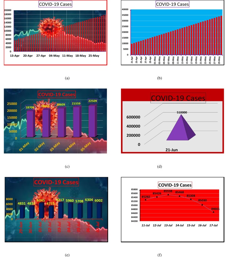
Yousaf et al. [20] performed statistical analysis for the month of May, for Pakistan, by using vector Auto Regressive Integrated Moving Average Model $(\mathit{ARIMA})$. According to their model prediction, the confirmed number of cases may increase up to 33,079 (Fig. 1 a). Chaudhry et al. [21] used the Social Sciences statistical package (SPSS) version 23 (IBM Corp., Armonk, NY), and forecast was given by utilizing a simple moving average method in time series modeler. In Pakistan, they predicted that active cases of COVID-19 may go over 35,000 at the end of May (Fig. 1b). Muhammad Aslam [22] used Kalman filter with ARIMA for COVID-19 pandemic in Pakistan. He gave prediction of five days from May 1, 2020 to May 5, 2020 (Fig. 1c). Dil et al. [23] predicted COVID-19 number of patients in the Eastern Mediterranean Region. They estimated that by the $20\mathit{th}$ June 2020, cases will shoot up to 510,000 (Fig. 1d). Vector Auto-regressive model has been used by Khan et al. [24] to predict COVID-19 cases in Pakistan. Their 10 days forecasting (June 29, 2020–July 8, 2020), is shown in Fig. 1e. Ahmad and Asad [25] used very efficient technique, artificial neural network, to predict 7 days (July 11, 2020–July 17, 2020) active cases of COVID-19 in Pakistan (Fig. 1f). Mathematical analysis and prediction of COVID-19 cases has been discussed in Pakistan by Ali et al. [26] and Ozair et al. [27]. Their prediction show the decline of COVID-19 in December, 2020. Many other efficient studies can be seen in the literature for the better understanding of COVID-19 pandemic and to design effective control strategies. For example Boccaletti et al. [28] discussed three scientific communities that may play vital role in controlling this pandemic. Atangana [29] proposed a mathematical model based on fractal-fractional differential and integral operators to discuss the indication of spread profile through statistical figures of Italy. Khan and Atangana [30] discussed the dynamics of COVID-19 appeared in China by construction the mathematical model having Atangana-Baleanu fractional derivative. Although face mask is the powerful tool to protect against COVID-19. However, hypercapnia has been recognized which is related to symptoms of fatigue, muscular weakness, discomfort, headaches as well as drowsiness. Ernestine Atangana and Abdon Atangana [31] provided the literature review in order to determine which type of face masks should be used to avoid re-inhaling rejected ${\mathit{CO}}_2$. Furthermore, mathematical models representing the transport of COVID-19 spread through wind has also been designed. The comprehensive statistical analysis of COVID-19 cases in Turkey and South Africa has been given by Abdon Atangana and Seda İğret Araz [32]. Recently, Atangana and Araz [33] utilized stochastic and deterministic approaches for forecasting of COVID-19 in Africa and Europe. The interested readers may also go through [34], [35], [36], [37]. To evaluate the dynamics of second wave, we modeled the transmission through a deterministic model SEIQR for COVID-19 infection in Pakistan.

Fig. 1.

Prediction of COVID-19 patients in Pakistan using various models and methods.

The Model structure

The whole population is distributed into five groups in the SEIQR style model, the susceptible $(S)$, exposed $(E)$, the infectious $(I)$, quarantine $(Q)$ and the recovered $(R)$. We suppose that susceptible humans are recruited at the rate $\mathrm{\Lambda }$ and leave the compartment through natural mortality rate as well as after getting infection. Humans belonging to all classes have natural mortality rate $\mu$. The class having COVID-19 infectious patients (I) has additional mortality rate $\eta$. Corona Virus is transmitted in susceptible humans, at the rate $\beta$, as a result of exposure of infectious humans with susceptible ones. Exposed individuals switch with the rate ${\alpha }_1$ to the infectious group. Transition of infectious individuals occurs at the rate $\gamma$. They move to either quarantine or recovered class. The portion $(1-\delta )$ of infectious individuals enter in the quarantine class (at the rate $\gamma$) and the remaining portion $\gamma \delta$, after recovery, join the recovered class. The detailed description of the parameters and their dimension is given in Table 1 . The assumption that people are homogeneously mixed leads to the following mathematical form of the model:

$$\begin{array}{cc}\hfill \frac{\mathit{dS}}{\mathit{dt}}=& \mathrm{\Lambda }-\beta \mathit{SI}-\mu S\hfill \\ \hfill \frac{\mathit{dE}}{\mathit{dt}}=& \beta \mathit{SI}-{\alpha }_{1}E-\mu E\hfill \\ \hfill \frac{\mathit{dI}}{\mathit{dt}}=& {\alpha }_{1}E-\left(\mu +\gamma +\eta \right)I\hfill \\ \hfill \frac{\mathit{dQ}}{\mathit{dt}}=& -\varphi Q-\mu Q+\gamma \left(1-\delta \right)I\hfill \\ \hfill \frac{\mathit{dR}}{\mathit{dt}}=& \varphi Q+\delta \gamma I-\mu R\text{.}\hfill \end{array}$$ (1)

with initial conditions $S(0)>0$ and $E(0),I(0),Q(0),R(0)⩾0$.

Table 1.

Definition, dimension of the model and parameter values (1).

Parameter	Description	Dimension
$\beta$	The effectual contact rate among susceptible and infectious individuals	day −1
$\mu$	Death rate of individuals (Natural)	day −1
${\alpha }_1$	The rate of exposed individuals becoming infectious	day −1
$\gamma$	The recovery rate of infected ones	day −1
$1-\delta$	The portion of infected individuals
	that are quarantined or recovers (at the rate $\gamma$)	dimensionless
$\delta$	The resting part of infected individuals who are quarantined	dimensionless
$\mathrm{\Lambda }$	The recruitment rate of susceptible individuals	day −1
$\varphi$	Quarantine rate of infections	day −1
$\eta$	Disease related death rate	day −1

Analysis of the model

Positively invariant set

We can easily verify that all classes of individuals ($S,E,I,Q,R$) are non-negative for all $t⩾0$ with non-negative initial conditions. Furthermore, the closed set

$$\mathrm{\Gamma }=\{(S,E,I,Q,R)\in R_{+}^5:S+E+I+Q+R⩽\frac{\mathrm{\Lambda }}{\mu }\}$$

is positively invariant.

Equilibrium points and basic reproduction number

The model has two types of equilibrium points, first one is disease free (DF), $E_0$, and second is endemic equilibrium (EE), $E^{\ast }$. We can write very easily our $E_0$, by simply putting the disease classes and derivatives equal to zero in (1), it would have the form $E_0=\left(\frac{\mathrm{\Lambda }}{\mu },0,0,0,0\right)$. The complete dynamics of the ailment is contingent on a threshold parameter, known as basic reproduction number, which is defined as the mean number of the secondary infections or secondary infections that are produced by an infected person during his total infectious period. By using this parameter, one can know that whether the disease persists in the community or not. With the help of next generation method [38], we derive the expression for basic reproduction number as

$$R_0=\frac{\mathrm{\Lambda }\beta {\alpha }_1}{\mu \left(\mu +{\alpha }_1\right)\left(\mu +\gamma +\eta \right)}\text{.}$$

For $R_0>1$, let $E^{\ast }$=$(S^{\ast },E^{\ast },I^{\ast },Q^{\ast },R^{\ast })$ be endemic equilibrium, where,

$$\begin{array}{cc}\hfill S^{\ast }=& \frac{\mathrm{\Lambda }}{\beta I^{\ast }+\mu }\hfill \\ \hfill E^{\ast }=& \frac{\beta I^{\ast }\mathrm{\Lambda }}{\left(\beta I^{\ast }+\mu \right)\left({\alpha }_1+\mu \right)}\hfill \\ \hfill Q^{\ast }=& \frac{\gamma \left(1-\delta \right)I^{\ast }}{\varphi +\mu }\hfill \\ \hfill R^{\ast }=& \frac{\left[\varphi \left(1-\delta \right)+\left(\varphi +\mu \right)\delta \right]\gamma I^{\ast }}{\left(\varphi +\mu \right)\mu }\hfill \\ \hfill I^{\ast }=& \frac{\mu }{\beta }\left(R_0-1\right)\text{.}\hfill \end{array}$$

Estimation of parameters

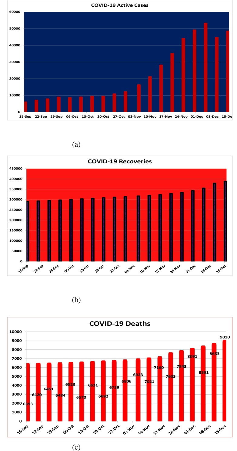
We estimate the values of parameters from available COVID-19 data and literature published. In given Fig. (2 ), only active cases with recovered ones and deaths have been plotted from ${15}^{\mathit{th}}$ of Sep., 2020 to December 15, 2020. Pakistan currently has a total population of nearly 220 millions [39] and life expectancy of 67 years [40]. Different studies show that the incubation time period for COVID-19 ranges from 2 to 14 days and almost $97.55\%$ people show disease symptoms within $11.5$ days of infection [41], [42], [43]. We estimate the remaining parameters by fitting the model with active number of COVID-19 patients. The second wave of Corona-virus appears in Pakistan on September 15, 2020. From that day, the COVID-19 patients have been continuously boosting up till December 6, 2020. It means that the peak period of second wave of the pandemic was $6\mathit{th}$ December. Now the number of active cases are decreasing day by day. So we divide the analysis in two phases. In the first phase, we estimate the number of cases by fitting the model with the increasing trend and in second phase, we calibrate our model results by the deceleration of number of active cases in Pakistan.

Fig. 2.

Number of COVID-19 patients, Recoveries and Deaths in Pakistan for second wave.

Phase-I

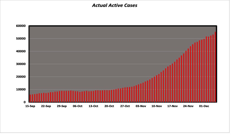
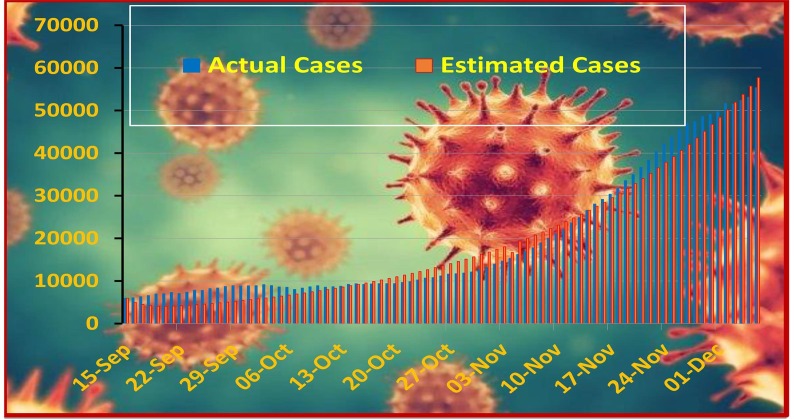
Here we study the increasing pattern of COVID-19 patients which starts from September 15, 2020 lasts up to December 7, 2020. Fig. (3) shows the number of actual cases that happened during the said period. We simulate the model and estimate the patients by finding suitable values of the parameters. The comparison between actual and fitted data is expressed in Fig. (4) . The estimated parameter values are shown in Table 2 .

Fig. 3.

Actual COVID-19 patients in Pakistan till December 7, 2020.

Fig. 4.

Comparison of actual and estimated cases of COVID-19 till December 7, 2020.

Table 2.

Definition, dimension of the model and parameter values (1).

Parameter	Description	Dimension	Value
$\beta$	The effectual contact rate among susceptible and infectious individuals	Day −1	2.43269 $\times {10}^{-9}$
$\mu$	Death rate of individuals (Natural)	day −1	0.0000408914
${\alpha }_1$	The rate of exposed individuals becoming infectious	day −1	0.0869565
$\gamma$	The recovery rate of infected ones	day −1	0.082
$1-\delta$	The portion of infected individuals that are quarantined or recovers (at the rate $\gamma$)	Dimensionless	0.131
$\delta$	The resting part of infected individuals who are quarantined	day −1	0.896
$\mathrm{\Lambda }$	The recruitment rate of susceptible individuals	day −1	8996.11
$\varphi$	Quarantine rate of infections	day −1	0.906
$\eta$	Disease related death rate	day −1	0.262

Phase-II

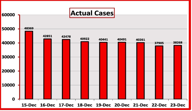
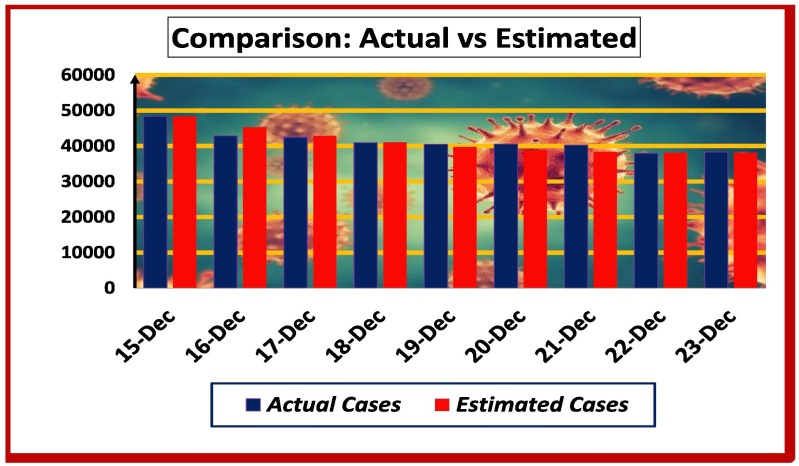
The decline in number of COVID-19 patients in Pakistan occurs after December 7, 2020. Small variation appears between December 8, 2020 and December 15, 2020. After this date, the pandemic is continuously disappearing. We again simulate the model by consider active cases of December 16 as the initial value and estimate the parameter values. Fig. (5) show the actual deceleration in number of patients of COVID-19 and Fig. (6) shows the fitting data with the actual cases. The values of estimated parameters is shown in Table 3 .

Fig. 5.

Actual Number of Patients from December 15 to 23.

Fig. 6.

Comparison of Estimated and Real Cases from December 15 to 23.

Table 3.

Definition, dimension of the mode and parameter values (1).

Parameter	Description	Dimension	Value
$\beta$	The effectual contact rate among susceptible and infectious individuals	day −1	00.000000000709267
$\mu$	Death rate of individuals (Natural)	day −1	0.0000408914
${\alpha }_1$	The rate of exposed individuals becoming infectious	day −1	00.0869565
$\gamma$	The recovery rate of infected individuals	day −1	00.0916795
$1-\delta$	The portion of infected individuals are quarantine or recovers (at the rate $\gamma$)	Dimensionless	00.12
$\delta$	The resting part of infected individuals who are quarantined	day −1	00.88
$\mathrm{\Lambda }$	The recruitment rate of susceptible individuals	day −1	8996.11
$\varphi$	Quarantine rate of infections	day −1	0.172
$\eta$	Disease related death rate	day −1	00.0000000000139611

Sensitivity analysis

To contemplate capacity of pandemic to get in a populace is our primary concern. Sensitivity analysis is carried out to analyse those factors due to which this malady disseminates and persists in the community. We target that parameters due to which larger deviation is produced in the value of basic reproduction number.

Sensitivity indices of $R_{\circ }$

The corresponding variance in the state variable, by the variation of a parameter, can be calculated through the sensitivity indices. Calculation of these indices has been made through the definition given in [44]. The sensitivity index is defined, in the form of partial derivatives, as given below:

$${\mathrm{\Gamma }}_p^x=\frac{\partial x}{\partial p}\times \frac{p}{x}\text{.}$$

By definition given above, the analytical formulas for the sensitivity indices of $R_{\circ }$ can be calculated. We can see from Table 4 that the parameter which shows most sensitivity is the adequate contact rate among susceptible and infectious individual followed by the recovery rate of infectious individuals. These indices indicate that if we able to enhance the recovery rate and reduce the adequate contact rate by almost 10%, the value of basic reproduction number may reduce up to 10%.

Table 4.

Sensitivity indices of $R_0$ corresponding to all parameters

Parameter	Sensitivity index	Parameter	Sensitivity index
$\mathrm{\Lambda }$	1	$\mu$	$1.00092$
${\alpha }_1$	$0.00047003$	$\beta$	1
$\gamma$	$-0.999554$	$\eta$	$1.522136984456319\times {10}^{-10}$

Reduction in basic reproduction number for different parameters

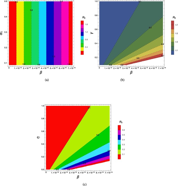
By using the parameter values given in Table (3), we plotted the reproduction number $R_0$ as a function of $\beta$ and $\alpha ,\beta$ and $\gamma ,\beta$ and $\eta$. Fig. (7a) shows the effect of effectual contact rate and incubation period of exposed patients on the reproduction number, we can see that these two parameters may decrease to $R_0$ less than unity if the value of $\beta$ remain up to $4\times {10}^{-10}$ and the incubation period remains between 2 and 14 days. The combined effect of transmission and recovery rate on $R_0$ is shown in Figs. (7b). As one parameter ($\beta$) is directly proportional and $\gamma$ is inversely related to $R_0$ so we can see that the basic reproduction number value may be reduced below unity even if the transmission rate $\beta$ approaches to $7\times {10}^{-10}$ and the infectious period increases to 5 days. Fig. (7c) shows the effect of transmission rate $\beta$ and $\eta$. We can see that these two parameters have considerable impact in reducing or increasing the value of basic reproduction number $R_0$.

Fig. 7.

Contour Plots of $R_{\circ }$ for different parameters.

Optimal control

Sensitivity analysis discussed in the previous section guides us to design effective control strategy in order to overcome this pandemic. As we applied the sensitivity analysis on the estimated parameters that have been obtained from the comparison of actual data and the outcomes of model. So, we can see almost clear picture of the future behaviour of this pandemic. By observing the most influential parameters, we reshape the model (1) to survey the influence of control measures regarding the future scenario. After inclusion of two controls, the model (1) gets the following form:

$$\begin{array}{cc}\hfill \frac{\mathit{dS}}{\mathit{dt}}=& \mathrm{\Lambda }-\beta (1-u_1)\mathit{SI}-\mu S,\hfill \\ \hfill \frac{\mathit{dE}}{\mathit{dt}}=& \beta (1-u_1)\mathit{SI}-{\alpha }_{1}E-\mu E-r_1{u}_{2}E,\hfill \\ \hfill \frac{\mathit{dI}}{\mathit{dt}}=& {\alpha }_{1}E-\left(\mu +\gamma +\eta \right)I,\hfill \\ \hfill \frac{\mathit{dQ}}{\mathit{dt}}=& \left(-\varphi Q-\mu Q+\gamma \left(1-\delta \right)I+r_1{u}_{2}E\right),\hfill \\ \hfill \frac{\mathit{dR}}{\mathit{dt}}=& \varphi Q+\delta \gamma I-\mu R\text{.}\hfill \end{array}$$ (2)

The control $u_1(t)$ represents the precautionary measures such as social distancing, abundant use of face mask etc. to reduce the transmission of infection into healthy people. Control $u_2(t)$ represents the quick action to isolate the people having COVID-19 virus. To discuss the ideal attempts to restraint the disease, we formulate the objective functional J. Its aim is to curtail the infectious individuals as well as the minimization of cost of applied controls $u_1$ and $u_2$. One has

$$J(u_1,u_2)={\int }_0^T(M_{1}E+M_{2}I+M_{3}Q+D_1{u}_1^2+D_2{u}_2^2)\mathit{dt},$$

where $M_1,M_2,M_3$ represent the positive weights. Our main objective is to curtail the number of infectious whilst reducing the cost of above mentioned controls with the help of described objective functional. Controls $u_1^{\ast }$ and $u_2^{\ast }$ can be found in such a way that

$$J(u_1^{\ast },u_2^{\ast })=\mathit{min}\{J(u_1,u_2),(u_1,u_2)\in U\},$$

in which, U, which is called control set, and is given by

$$U=\{(u_1,u_2)|u_i(t)\mathit{isLebsguemeasurableon}[0,1],0⩽u_i(t)⩽1,i=1,2\}\text{.}$$

By the use of Pontryagin’s Maximum Principle [45], we can have the essential conditions and solution of (2).

Existence and analysis for optimal control

The existence and analysis of an optimal control could be verified with the help of powerful classical procedure. According to [46], it is necessary to check that the following hypotheses hold:

$(H_1)$ Controls set and corresponding described variables is nonempty.

$(H_2)$ U must fulfills the two properties the convexity and closeness.

$(H_3)$ Right hand side of the described system is bounded by a linear function in the control state.

$(H_4)$ Objective functional J has convex integrand on U and bounded below by $c_1{({\sum }_{i=1}^3|u_i{|}^2)}^{\frac{\tau }{2}}-c_2$ , where $c_1,c_2>0$ and $\tau >1$.

The result in Lukes ([47], Th 9.2.1, p 182) is utilized for existence of solutions of system (2). In this way, we verify the above hypothesis. $(H_1)$ is satisfied due to boundedness of coefficients and solutions, boundedness shows that U fulfils the second hypothesis. As the system (2) is bilinear in $u_1,u_2$ and due to the boundedness of solutions, right hand side of (2) fulfils the third hypothesis $H_3$. Since the control functions $u_1$ and $u_2$ are convex and number of infectious hosts and vectors are also bounded at any time t by the positivity of solutions, so we can choose constants $M_1,M_2,M_3,D_1,D_2,c_1,c_2$ all are positive and $\tau >1$ such that the inequality

$$M_{1}E+M_{2}I+M_{3}Q+D_1{u}_1^2+D_2{u}_2^2⩾c_1{({\displaystyle \sum _{i=1}^2}|u_i{|}^2)}^{\frac{\tau }{2}}-c_2,$$

is satisfied. Thus the last condition is also verified. So, we have the theorem given below:

Theorem 1

For objective functional $J(u_1,u_2)={\int }_0^T(M_{1}E+M_{2}I+M_{3}Q+D_1{u}_1^2+D_2{u}_2^2)\mathit{dt}$ where $U=\{(u_1,u_2)|0⩽u_1,u_2\le 1,t\in [0,T]$ subject to Eqs. (2) with initial conditions, there exists an optimal control $u=(u_1^{\ast },u_2^{\ast })$ so that $J(u_1^{\ast },u_2^{\ast })=\mathit{min}\{J(u_1,u_2),(u_1,u_2)\in U\}$.

If we can have the Lagrangian and Hamiltonian of the system (2), then one can get the optimal solution. Lagrangian, for (2), is given by

$$\mathbb{L}(I_h,I_v,u_1,u_2)=M_{1}E+M_{2}I+M_{3}Q+D_1{u}_1^2+D_2{u}_2^2⩾c_1(|u_1{|}^2+|u_2{|}^2\text{.}$$

One has to build up the least possible value $\mathbb{L}$ given above. To get objective, we have to define the Hamiltonian H in this way:

Let us consider $X=(S,E,I,Q,R),\lambda =({\lambda }_1,{\lambda }_2,{\lambda }_3,{\lambda }_4,{\lambda }_5)$ and $U=(u_1,u_2)$, so we have:

$$\begin{array}{c}\hfill H(X,U,\lambda )=M_{1}E+M_{2}I+M_{3}Q+D_1{u}_1^2+D_2{u}_2^2+{\lambda }_1\left(\mathrm{\Lambda }-\beta (1-u_1)\mathit{SI}-\mu S\right)\\ \hfill +{\lambda }_2\left(\beta (1-u_1)\mathit{SI}-{\alpha }_{1}E-\mu E-r_1{u}_{2}E\right)+{\lambda }_3\left({\alpha }_{1}E-\left(\mu +\gamma +\eta \right)I\right)\\ \hfill +{\lambda }_4\left(-\varphi Q-\mu Q+\gamma \left(1-\delta \right)I+r_1{u}_{2}E\right)+{\lambda }_5\left(\varphi Q+\delta \gamma I-\mu R\right)\text{.}\end{array}$$

The optimality system

Maximum Principle explored by Pontryagin as reported in [48] is used for finding essential optimal control conditions. This is calculated as follows:

For optimized solution $(u_1^{\ast },u_2^{\ast })$ of optimal control problem (2), a vector function $\lambda (t)=({\lambda }_1(t),\dots ,{\lambda }_5(t))$, which is nontrivial, prevails that fulfils the ensuing conditions. The stated relation is

$$\frac{\mathit{dx}}{\mathit{dt}}=\frac{\partial }{\partial \lambda }(H(t,U^{\ast },\lambda (t))),$$

$$0=\frac{\partial }{\partial u}(H(t,U^{\ast },\lambda (t))),$$

$$\frac{d\lambda }{\mathit{dt}}=-\frac{\partial }{\partial x}(H(t,U^{\ast },\lambda (t)))\text{.}$$

Now, mandatory conditions are incorporated for H.

Theorem 2

For $U^{\ast }(u_1^{\ast },u_2^{\ast })$ and solutions $(S,E,I,Q,R)$ of the system (2) , variables ${\lambda }_1,\dots ,{\lambda }_5$ occurs having,

$$\begin{array}{cc}\hfill \frac{d{\lambda }_1}{\mathit{dt}}=& \left({\lambda }_2-{\lambda }_1\right)\beta (1-u_1)I+{\lambda }_1\mu ,\hfill \\ \hfill \frac{d{\lambda }_2}{\mathit{dt}}=& -M_1+{\lambda }_2({\alpha }_1+\mu +r_1{u}_2)-{\lambda }_3{\alpha }_1-{\lambda }_4{r}_1{u}_2,\hfill \\ \hfill \frac{d{\lambda }_3}{\mathit{dt}}=& -M_2+\left({\lambda }_2-{\lambda }_1\right)\beta (1-u_1)S+{\lambda }_3\left(\mu +\gamma +\eta \right)-{\lambda }_4\gamma \left(1-\delta \right)-{\lambda }_5\delta \gamma ,\hfill \\ \hfill \frac{d{\lambda }_4}{\mathit{dt}}=& -M_3+{\lambda }_4\left(\varphi +\mu \right),\hfill \\ \hfill \frac{d{\lambda }_5}{\mathit{dt}}=& {\lambda }_5\mu ,\hfill \end{array}$$

with transversality conditions ${\lambda }_1(T)={\lambda }_2(T)=\dots ={\lambda }_5(T)$ . Additionally, $u_1^{\ast },u_2^{\ast }$ are expressed as

$$\begin{array}{cc}\hfill u_1^{\ast }=& \max \{\min \{1,\{\frac{\beta \mathit{SI}({\lambda }_2-{\lambda }_1)}{D_1}\},0\},\hfill \\ \hfill u_2^{\ast }=& \max \{\min \{1,\frac{({\lambda }_2-{\lambda }_4)r_{1}E}{D_2}\},0\}\text{.}\hfill \end{array}$$

Proof

By making use of H, we can get the adjoint equations and the transversality conditions. Set $S=S^{\ast },E=E^{\ast },I=I^{\ast },Q=Q^{\ast },R=R^{\ast }$ and differentiate the Hamiltonian H with respect to variables $S,E,I,Q,R$. Hence we have

$$\begin{array}{cc}\hfill \frac{d{\lambda }_1}{\mathit{dt}}=& \left({\lambda }_2-{\lambda }_1\right)\beta (1-u_1)I+{\lambda }_1\mu ,\hfill \\ \hfill \frac{d{\lambda }_2}{\mathit{dt}}=& -M_1+{\lambda }_2({\alpha }_1+\mu +r_1{u}_2)-{\lambda }_3{\alpha }_1-{\lambda }_4{r}_1{u}_2,\hfill \\ \hfill \frac{d{\lambda }_3}{\mathit{dt}}=& -M_2+\left({\lambda }_2-{\lambda }_1\right)\beta (1-u_1)S+{\lambda }_3\left(\mu +\gamma +\eta \right)-{\lambda }_4\gamma \left(1-\delta \right)-{\lambda }_5\delta \gamma ,\hfill \\ \hfill \frac{d{\lambda }_4}{\mathit{dt}}=& -M_3+{\lambda }_4\left(\varphi +\mu \right),\hfill \\ \hfill \frac{d{\lambda }_5}{\mathit{dt}}=& {\lambda }_5\mu \text{.}\hfill \end{array}$$

with transversality conditions ${\lambda }_1(T)={\lambda }_2(T)=\dots {\lambda }_5(T)=0$. Optimality conditions and the property set U of controls give the result

$$\begin{array}{cc}\hfill u_1^{\ast }=& \max \{\min \{1,\{\frac{\beta \mathit{SI}({\lambda }_2-{\lambda }_1)}{D_1}\},0\},\hfill \\ \hfill u_2^{\ast }=& \max \{\min \{1,\frac{({\lambda }_2-{\lambda }_4)r_{1}E}{D_2}\},0\}\text{.}\hfill \end{array}$$

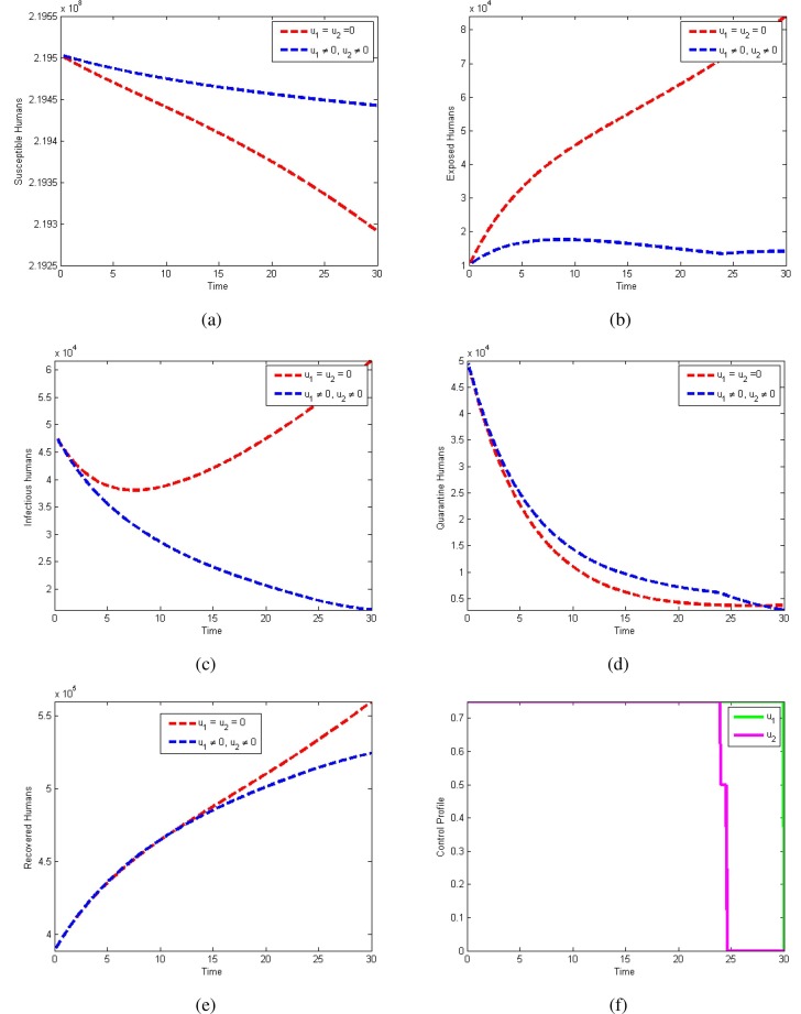
Outcome of the optimal controls on the transmission of COVID-19 can also be observed numerically. Horizontal axes represent time in days and vertical axes indicates individuals in the specific compartment. we start the control from December 16, 2020. The actual number of COVID-19 patients was $~48,369$. We take this number as an initial value and simulate the modified model for next 30 days. In Fig. 8a , we observe that the number of susceptible humans increases by applying the controls. Fig. 8b shows that the persons having Corona-virus decreases by applying the controls. Fig. 8c also represents the significant reduction in the number of infectious by adopting the control measures. There will be no considerable difference in the number of quarantined individuals. However, Fig. 8d shows that they decrease after 27 days. Fig. 8e shows that recovered people will decrease by applying the controls. It will happen due to significant reduction in the number of exposed and infectious individuals in the coming days. Control profile is shown in Fig. 8f. It shows that, to get the huge reduction in the pandemic, we have to apply both controls with almost $80\%$ efficacy.

Fig. 8.

Use of Controls $u_1$ and $u_2$.

Conclusions

In this study, we have interpreted the deterministic COVID-19 disease model carefully to determine the feasibility of emergence of COVID-19 patients throughout Pakistan. We compared the result of our model with the actual confirmed cases, it has been noted that there is appropriate correspondence between estimated values and actual confirmed numbers. If the current scenario is continuing then, according to our estimation, the active number of COVID-19 cases will decrease gradually. However, the scenario will change by the changing of parameters.

The model has been analyzed qualitatively. Explicit formula for the reproduction number has been calculated. Two types of equilibria, disease free and endemic, has been calculated. The model has been applied on the second wave of COVID-19 in Pakistan. We fitted the model both for increasing and decreasing pattern of COVID-19 data. The parameters have been estimated through the calibration of real data. Active patients in Pakistan are decreasing gradually for past few days. So we focus our analysis on the recent trend.

The parameters having vital impacts on the basic reproduction number have been identified. This sensitivity analysis has been performed by using the numerical values of the parameters obtained through fitting of the model with actual number of active cases showing decreasing pattern. First we calculate the sensitivity indices of basic reproduction number with respect to all the parameters. It has been observed that the most sensitive parameter (ignoring the sensitivity indices of demographic parameters) is the adequate contact rate among susceptible and infectious humans. Secondly, we observed the combined effect of every two parameters on the basic reproduction number.

On the basis of measuring sensitivity, we modified the formulated mathematical model by introducing the control functions. First is the attempt to maintain the social distancing or keeping the practice of wearing face mask and second is the quick action of making the quarantine of infected people. We numerically solve the optimal control problem. It has been calculated that, by the application of control measures, the number of exposed and infectious individuals will be $~14,260$ and $~16,210$, respectively. However, these numbers may increase up to $~83,420$ and $~61,700$, respectively, till the end of January, 2021, if proper interventions have not been applied. In future, we shall try to prove the global stability of disease free equilibrium as well as endemic equilibrium and, through the parameter calibration, we shall estimate the constant maximum number of COVID-19 patients for both cases that is for disease persistence and disease extinction. Mathematical model can also be modified for example by the addition of hospitalized class.

Declaration of Competing Interest

The authors declare that they have no known competing financial interests or personal relationships that could have appeared to influence the work reported in this paper.

References

- 1.Izquierdo L.D. Diss. Instituto de Salud Carlos III; 2020. INFORME TÉCNICO Nuevo coronavirus 2019-nCoV. [Google Scholar]
- 2.W.H. Organization. Novel coronavirus (2019-ncov) situation reports; 2020. URL: https://www.who.int/emergencies/diseases/novel-coronavirus-2019/situation-reports.
- 3.Paules C.I., Marston H.D., Fauci A.S. Coronavirus infections-more than just the common cold. Jama. 2020;323(8):707–708. doi: 10.1001/jama.2020.0757. [DOI] [PubMed] [Google Scholar]
- 4.Saif L.J. Animal coronavirus vaccines: lessons for SARS. Develop Biol. 2004;119:129–140. [PubMed] [Google Scholar]
- 5.https://www.pakistantoday.com.pk/2020/02/26/sindh-health-two-coronavirus-cases-confirmed-in-pakistan-confirms-first-coronavirus-case-in-karachi.
- 6.Alnaser W.E., Abdel-Aty M., Al-Ubaydli O. Mathematical prospective of coronavirus infections in Bahrain, Saudi Arabia and Egypt. Inf Sci Lett. 2020;9(1):51–64. [Google Scholar]
- 7.http://covid.gov.pk/.
- 8.https://www.worldometers.info/coronavirus/country/pakistan/.
- 9.Rida Saad Z., Farghaly Ahmed A., Azoz Shaimaa A. Fatma Hussien Global stability of a delayed fractional-order SEI epidemic model with logistic growth. Appl Math Inf Sci. 2021;15(1):31–42. [Google Scholar]
- 10.Abdel-Aty A.-H., Khater M.M.A., Dutta H., Bouslimi J., Omri M. Computational solutions of the HIV-1 infection of CD4+T-cells fractional mathematical model that causes acquired immunodeficiency syndrome (AIDS) with the effect of antiviral drug therapy. Chaos Solitons Fractals. 2020;139 doi: 10.1016/j.chaos.2020.110092. [DOI] [PMC free article] [PubMed] [Google Scholar]
- 11.Saravanakumar S., Eswari A., Rajendran L., Abukhaled M. A mathematical model of risk factors in HIV/AIDS transmission dynamics: observational study of female sexual network in India. Appl Math Inf Sci. 2020;14(6):967–976. [Google Scholar]
- 12.Das U.D., Singh B.P., Roy T.D. Temporal variation of temperature in Guwahati, Assam: an application of seasonal ARIMA model. J Stat Appl Prob. 2020;9(1):169–180. [Google Scholar]
- 13.Jardón-Kojakhmetov H., Kuehn C., Pugliese A., Sensi M. A geometric analysis of the SIR, SIRS and SIRWS epidemiological models. Nonlinear Anal: Real World Appl. 2020;58 [Google Scholar]
- 14.Wu J.T., Leung K., Leung G.M. Nowcasting and forecasting the potential domestic and international spread of the 2019-nCoV outbreak originating in Wuhan, China: a modelling study. Lancet. 2020;395(10225):689–697. doi: 10.1016/S0140-6736(20)30260-9. [DOI] [PMC free article] [PubMed] [Google Scholar]
- 15.Ullah A., Ahmad S., Owyed S., Abdel-Aty A.H., Mahmoud E.E., Shah K., Alrabaiah H. Mathematical analysis of COVID-19 via new mathematical model. Chaos Solitons Fractals. 2020;143(2021) doi: 10.1016/j.chaos.2020.110585. [DOI] [PMC free article] [PubMed] [Google Scholar]
- 16.Abdulwasaa M.A., Abdo M.S., Shah K., Nofal T.A., Panchal S.K., Kawale S.V., Abdel-Aty A.-H. Fractal-fractional mathematical modeling and forecasting of new cases and deaths of COVID-19 epidemic outbreaks in India. Results Phys. 2021;20 doi: 10.1016/j.rinp.2020.103702. [DOI] [PMC free article] [PubMed] [Google Scholar]
- 17.Shahzad M., Abdel-Aty A.-H., Attia R.A.M., Khoshnaw S.H.A., Aldila D., Ali M., Sultan F. Dynamics models for identifying the key transmission parameters of the COVID-19 disease. Alexandria Eng J. 2021;60(1):757–765. [Google Scholar]
- 18.Kermack W.O., McKendrick A.G. A contribution to the mathematical theory of epidemics. Proc R Soc London Ser A. 1927;115(772):700–721. [Google Scholar]
- 19.Brauer F., Castillo-Chavez C., Feng Z. vol. 32. Springer; New York: 2019. (Mathematical models in epidemiology). [Google Scholar]
- 20.Yousaf M., Zahir S., Riaz M., Hussain S.M., Shah K. Statistical analysis of forecasting COVID-19 for upcoming month in Pakistan. Chaos Solitons Fractals. 2020;138 doi: 10.1016/j.chaos.2020.109926. [DOI] [PMC free article] [PubMed] [Google Scholar]
- 21.Chaudhry R.M., Hanif A., Chaudhary M., Minhas S. Coronavirus Disease 2019 (COVID-19): Forecast of an Emerging Urgency in Pakistan. Cureus. 2020;12(5) doi: 10.7759/cureus.8346. [DOI] [PMC free article] [PubMed] [Google Scholar]
- 22.Aslam M. Using the Kalman filter with ARIMA for the COVID-19 pandemic dataset of Pakistan. Data Brief. 2020;105854 doi: 10.1016/j.dib.2020.105854. [DOI] [PMC free article] [PubMed] [Google Scholar]
- 23.Dil S., Dil N., Maken Z.H. COVID-19 trends and forecast in the Eastern Mediterranean Region with a Particular Focus on Pakistan. Cureus. 2020;12(6) doi: 10.7759/cureus.8582. [DOI] [PMC free article] [PubMed] [Google Scholar]
- 24.Khan F., Saeed A., Ali S. Modelling and forecasting of new cases, deaths and recover cases of COVID-19 by using vector autoregressive model in Pakistan. Chaos Solitons Fractals. 2020;140 doi: 10.1016/j.chaos.2020.110189. [DOI] [PMC free article] [PubMed] [Google Scholar]
- 25.Ahmad I., Asad S.M. Predictions of coronavirus COVID-19 distinct cases in Pakistan through an artificial neural network. Epidemiol Infect. 2020;148 doi: 10.1017/S0950268820002174. [DOI] [PMC free article] [PubMed] [Google Scholar]
- 26.Ali M., Imran M., Khan A. Analysis and Prediction of the COVID-19 outbreak in Pakistan. J Biol Dyn. 2020;14(1):730–747. doi: 10.1080/17513758.2020.1814883. [DOI] [PubMed] [Google Scholar]
- 27.Ozair M., Hussain T., Hussain M., Awan A.U., Baleanu D., Abro K.A. A mathematical and statistical estimation of potential transmission and severity of COVID-19: a combined study of Romania and Pakistan. BioMed Res Int. 2020;2020 doi: 10.1155/2020/5607236. [DOI] [PMC free article] [PubMed] [Google Scholar]
- 28.Boccaletti S., Ditto W., Mindlin G., Atangana A. Modeling and forecasting of epidemic spreading: the case of Covid-19 and beyond. Chaos Solitons Fractals. 2020;135 doi: 10.1016/j.chaos.2020.109794. [DOI] [PMC free article] [PubMed] [Google Scholar]
- 29.Atangana A. Modelling the spread of COVID-19 with new fractal-fractional operators: can the lockdown save mankind before vaccination? Chaos Solitons Fractals. 2020;136 doi: 10.1016/j.chaos.2020.109860. [DOI] [PMC free article] [PubMed] [Google Scholar]
- 30.Khan M.A., Atangana A. Modeling the dynamics of novel coronavirus (2019-nCov) with fractional derivative. Alexandria Eng J. 2020;59(4):2379–2389. [Google Scholar]
- 31.Atangana E., Atangana A. Facemasks simple but powerful weapons to protect against COVID-19 spread: can they have sides effects? Results Phys. 2020;103425 doi: 10.1016/j.rinp.2020.103425. [DOI] [PMC free article] [PubMed] [Google Scholar]
- 32.Atangana A., Araz S.İ. Mathematical model of COVID-19 spread in Turkey and South Africa: theory, methods, and applications. Adv Differ Equ. 2020;2020(1):1–89. doi: 10.1186/s13662-020-03095-w. [DOI] [PMC free article] [PubMed] [Google Scholar]
- 33.Atangana A., Araz S.İ. Modeling and forecasting the spread of COVID-19 with stochastic and deterministic approaches: Africa and Europe. Adv Differ Equ. 2021;2021(1):1–107. doi: 10.1186/s13662-021-03213-2. [DOI] [PMC free article] [PubMed] [Google Scholar]
- 34.Shaikh A.S., Shaikh I.N., Nisar K.S. A mathematical model of COVID-19 using fractional derivative: outbreak in India with dynamics of transmission and control. Adv Differ Equ. 2020;2020(1):1–19. doi: 10.1186/s13662-020-02834-3. [DOI] [PMC free article] [PubMed] [Google Scholar]
- 35.Nisar K.S., Ahmad S., Ullah A., Shah K., Alrabaiah H., Arfan M. Mathematical analysis of SIRD model of COVID-19 with Caputo fractional derivative based on real data. Results Phys. 2020;103772 doi: 10.1016/j.rinp.2020.103772. [DOI] [PMC free article] [PubMed] [Google Scholar]
- 36.Cheema S.A., Kifayat T., Rahman A.R., Khan U., Zaib A., Khan I., Nisar K.S. Is Social Distancing, and Quarantine Effective in Restricting COVID-19 Outbreak? Statistical Evidences from Wuhan, China. Comput Mater Continua. 2020;66(2) [Google Scholar]
- 37.Baba I.A., Yusuf A., Nisar K.S., Abdel-Aty A.H., Nofal T.A. Mathematical model to assess the imposition of Lockdown during COVID-19 pandemic. Results Phys. 2020;103716 doi: 10.1016/j.rinp.2020.103716. [DOI] [PMC free article] [PubMed] [Google Scholar]
- 38.Van den Driessche P., Watmough J. Reproduction numbers and sub-threshold endemic equilibria for compartmental models of disease transmission. Math Biosci. 2002;180(1–2):29–48. doi: 10.1016/s0025-5564(02)00108-6. [DOI] [PubMed] [Google Scholar]
- 39.https://www.macrotrends.net/countries/PAK/pakistan/population.
- 40.https://www.macrotrends.net/countries/PAK/pakistan/life-expectancy.
- 41.Lauer S.A., Grantz K.H., Bi Q., Jones F.K., Zheng Q., Meredith H.R., Lessler J. The incubation period of coronavirus disease 2019 (COVID-19) from publicly reported confirmed cases: estimation and application. Ann Internal Med. 2020;172(9):577–582. doi: 10.7326/M20-0504. [DOI] [PMC free article] [PubMed] [Google Scholar]
- 42.Lai C.C., Shih T.P., Ko W.C., Tang H.J., Hsueh P.R. Severe acute respiratory syndrome coronavirus 2 (SARS-CoV-2) and coronavirus disease-2019 (COVID-19): the epidemic and the challenges. Int J Antimicrob Agents. 2020;55(3) doi: 10.1016/j.ijantimicag.2020.105924. [DOI] [PMC free article] [PubMed] [Google Scholar]
- 43.Del Rio C., Malani P.N. COVID-19–new insights on a rapidly changing epidemic. Jama. 2020;323(14):1339–1340. doi: 10.1001/jama.2020.3072. [DOI] [PubMed] [Google Scholar]
- 44.Chitnis N., Hyman J.M., Cushing J.M. Determining important parameters in the spread of malaria through the sensitivity analysis of a mathematical model. Bull Math Biol. 2008;70(5):1272. doi: 10.1007/s11538-008-9299-0. [DOI] [PubMed] [Google Scholar]
- 45.Pontryagin L.S., Boltyanskii V.G., Gamkrelidze R.V., Mishchenko E.F. vol. 4. Gordon and Breach Science Publishers; New York, NY, USA: 1986. (The mathematical theory of optimal processes). [Google Scholar]
- 46.Fleming W.H., Rishel R.W. Springer; New York: 1975. Deterministic and stochastic optimal control. [Google Scholar]
- 47.Lukes D.L. Academic Press; New York: 1982. Differential equations: classical to controlled, mathematics in science and engineering. [Google Scholar]
- 48.Lenhart S., Workman J.T. Chapman and Hall/CRC Press; London/Boca Raton: 2007. Optimal control applied to biological models, Mathematical and Computational Biology Series. [Google Scholar]