A biologist's guide to model selection and causal inference

Abstract

A goal of many research programmes in biology is to extract meaningful insights from large, complex datasets. Researchers in ecology, evolution and behavior (EEB) often grapple with long-term, observational datasets from which they construct models to test causal hypotheses about biological processes. Similarly, epidemiologists analyse large, complex observational datasets to understand the distribution and determinants of human health. A key difference in the analytical workflows for these two distinct areas of biology is the delineation of data analysis tasks and explicit use of causal directed acyclic graphs (DAGs), widely adopted by epidemiologists. Here, we review the most recent causal inference literature and describe an analytical workflow that has direct applications for EEB. We start this commentary by defining four distinct analytical tasks (description, prediction, association, causal inference). The remainder of the text is dedicated to causal inference, specifically focusing on the use of DAGs to inform the modelling strategy. Given the increasing interest in causal inference and misperceptions regarding this task, we seek to facilitate an exchange of ideas between disciplinary silos and provide an analytical framework that is particularly relevant for making causal inference from observational data.

1. Introduction

In 1976, George Box noted, ‘All models are wrong' [1]. Yet, studies of cells to society require models to summarize data and draw inference, leaving researchers between the Scylla of imperfect models and the Charybdis that is the foundational role of models to evidence-based science.

In this commentary, we describe a methodical approach to model selection, data analysis and results interpretation that entails clear delineation of data science tasks in order to identify the appropriate analytical strategy, and emphasize the importance of prior knowledge to inform model selection when the goal of analysis is to make causal inference. While all scientific fields may benefit from a thoughtful and systematic analytical approach, the target audience is scientists in the ecology, evolution and behavior (EEB) discipline—a field that draws causal conclusions, often from observational data, in pursuit of proximate and ultimate explanations [2]. Nota bene, EEB scientists have extensive quantitative training, so giving a tutorial on specific statistical techniques is not our goal. Rather, we integrate and expand upon analytical paradigms used in epidemiology—another quantitative field that grapples with complex observational datasets—so that even when a model is not 100% correct, it improves scientific knowledge.

We start by describing four distinct data analysis tasks: description, prediction, association and causal inference. Then, we delve further into causal inference, a concept that is not new in EEB [3,4], but has experienced a recent resurgence of interest and is highly relevant to the types of data collected and analysed in this field [5–8]. Beyond providing guidelines for an analytical framework, a broader theme of this interdisciplinary piece is to harness synergy between two historically distinct disciplines—EEB and epidemiology—in order to promote multidisciplinary team science.

2. Data analysis tasks

Identifying the appropriate analytical task for a research question is the critical first step. Table 1 summarizes four distinct analytical tasks that may be used together or as stand-alone analyses: description, prediction, association and causal inference [9,10]. A distinguishing characteristic among the analytical tasks is the need for causal knowledge when formulating the modelling approach. Description and prediction do not necessarily require investigators to know the causal or temporal relationships beforehand, but prior causal knowledge is relevant to associational analyses and foundational to causal inference. We provide details on description, prediction and association in the electronic supplementary material (see electronic supplementary material, §1). In the main text, we focus on causal inference in the context of observational studies.

Table 1. Data analysis tasks.

task	key characteristics and concepts	example analytical tools/methods	causal knowledge needed?	example question	example verbiage & interpretation
description	A quantitative overview of the data. The metrics of interest may range from simple descriptive statistics to complex visualization techniques.	mean ± s.d., box plots, proportions, unsupervised cluster analyses, time trends, generalized regressiona	no	What is the central tendency and spread of T-cell count, a marker of immune function, in wild spotted hyenas in Kenya?	Summarize a feature based on the metric of interest. This includes but is not limited to: prevalence of a phenomenon (%, proportions), central tendency and dispersion (mean ± s.d., median, minimum, maximum), natural correlations among groups of variables (clusters or latent constructs), and/or trends in a variable over time (e.g. average rate of increase per year). Ex: In wild spotted hyenas, the median (range) T-cell count is 850 cells/mm2 (range: 500 to 1,200 cells/mm2).
prediction	Identification of a set of explanatory variables that optimize variation explained in a dependent variable, with no focus on the causal or temporal structure among the explanatory variables of interest. This task often involves use of automated procedures to maximize model fit and leverages the joint distribution of multiple variables.	tree-based techniques, recurrent neural networks, unsupervised machine learning algorithms, generalized regressiona	some	What set of social and ecological factors explain maximum variation in T-cell count in wild spotted hyenas in Kenya?	This task focuses on how well a set of X-variables (predictors) maximize variance in (predict) Y. Interpretation for individual X-variables focuses on assessments of model fit (e.g. AIC/BIC or adjusted R2), or predictive capacity (e.g. area under the receiver operating characteristic curve [AUC]) rather than a causal effect.). Ex: In wild spotted hyenas, a model that includes prey density, average yearly rainfall, and social rank as predictors of T-cell count yields the best model fit (lowest AIC and BIC, and/or highest adjusted R2) in comparison to other combinations of predictors derived from available data.
association	Assessment of the unadjusted relationship between two variables of interest. This relationship may be explored within strata of a few key other variables that may influence the association of interest and can inform future causal inference studies.	Pearson or Spearman correlation coefficients, estimates from unadjusted generalized regressiona	some	How does social connectedness correlate with T-cell count in wild spotted hyenas in Kenya?	Use non-causal language to describe the crude relationship between X and Y. The estimate for X can be interpreted as an association or relation or correlation, but not a causal effect.). Ex: Higher social connectedness is associated with higher T-cell count in wild spotted hyenas.
causal inference	Obtain a causal (i.e. unbiased) effect of X on Y. This type of analysis requires knowledge on the causal and temporal relationship between X and Y, as well as third variables (confounders, mediators, effect modifiers, colliders) that may influence this relationship in order to control bias.	use of directed acyclic graphs to reflect the research question, followed by an appropriate analytical strategy which can involve but are not limited to generalized regressiona, inverse probability weighting, structural equation modelling, path analysis, Rubin causal inference, and G-methods.	yes	Does social connectedness affect T-cell count in wild spotted hyenas in Kenya?	Causal interpretation of the relationship between X and Y via use of words such as ‘effect' to describe the relationship between X and Y, or ‘affect’ or ‘cause’ to indicate whether and how X influences Y. Ex: There is a direct positive effect of social connectedness on T-cell count in wild spotted hyenas.

^aIncludes generalized regression models (e.g. linear, Poisson, negative binomial, logistic) and generalized mixed models (e.g. linear mixed models, segmented mixed models, mixed models with splines).

3. Causal inference

The goal of causal inference is to quantify the effect of X on Y. The gold standard for this task is a randomized experiment or trial in which the process of randomization ensures equal distribution of underlying characteristics within the population such that the only difference between the treatment and control groups is the intervention. Accordingly, any difference in the outcome may be attributed to an effect of the intervention. However, experimentation is often not financially or ethically possible, and scientists remain interested in testing hypotheses and inferring causation from observational data. Counter to popular belief that specific techniques must be used to conduct causal inference analysis on observational data, the foundation of this task lies in an a priori focus on the specific relationship between X and Y, and consideration of additional third variables that can introduce bias. Techniques that are often associated with causal inference (e.g. structural equations modelling and/or path analysis [11], inverse probability weighting [12], G-methods [13]) relax assumptions of parametric regression models in order to reduce biases that transpire from statistical adjustment in regression models.

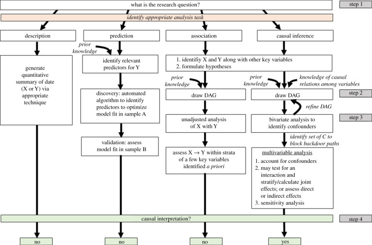
The concept of causal inference is not new in EEB, but the use of causal diagrams to inform model selection is a valuable epidemiological tool that has not penetrated EEB, with a few exceptions [6,7]. Here, we provide guidelines for making causal inference using directed acyclic graphs (DAGs). Figure 1 shows an analytical roadmap to making causal inference, as well as the other three tasks.

Figure 1.

Data analysis tasks and modelling approaches.

(a). Step 1: formulate the research question

Causal inference begins with a precise and specific research question which should reflect a testable hypothesis. A clear hypothesis for causal inference should be translatable into a contrast of counterfactual outcomes—i.e. what Y would be had X been different in a population. This requires identification of X and Y, specification of how each variable will be parameterized (i.e. discrete versus continuous) [14] and identification of the study population from which data are available for X and Y, as well as other variables that warrant consideration in the analysis, including confounders, precision covariates, mediators and effect modifiers.

(b). Step 2: draw the directed acyclic graph

A causal directed acyclic graph (DAG) is a flowchart that maps out the causal and temporal relationship between X and Y, along with additional variables that may affect the X → Y association. As such, a DAG is also a graphical representation of the hypothesis and a summary of the modelling approach [15,16].

The first step to drawing a DAG is to identify the X (cause) and Y (outcome) of interest. If our hypothesis is that social connectedness (number of affiliative interactions an individual has within their social network) affects immune function (T-cell count), then the corresponding DAG should show an arrow emerging from social connectedness pointing toward immune function (figure 2). This DAG translates into an unadjusted statistical model in which social connectedness is the explanatory variable and immune function is the dependent variable.

Figure 2.

DAG showing the causal relationship between X and Y.

While such a DAG and corresponding statistical model are straightforward, estimating the causal effect of X on Y often involves consideration of other variables that can introduce bias or modify the relationship of interest.

(i). Confounder

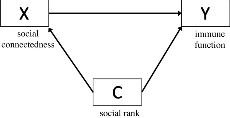
After defining the relationship of interest, the next step is to pinpoint sources of bias. One source of bias is confounders, or shared common causes of X and Y, denoted in a DAG as C with two arrows pointing at X and Y (figure 3). Confounders are identified via prior knowledge in conjunction with evidence of a statistical association of C with X and Y in the study sample, and should typically be accounted for in order to obtain an unbiased causal effect of X on Y.

Figure 3.

DAG showing the relationship between X and Y, with confounder C.

When a confounder is present, there are two paths through which the effect of X may flow to Y: (i) from X directly towards Y; and (ii) through a ‘backdoor path' that represents non-causal variation in the relationship between X and Y transpiring from a shared common cause, C. If the investigator is interested in the effect represented by the first arrow, then the backdoor path leads to confounding and should be ‘blocked' in order to obtain a causal estimate of X. Neglecting to do so may lead to biased estimates or worse, spurious associations [17]. The most common approach to control for confounding is to include the variable as a covariate in a regression model (statistical adjustment).

In our running example, social rank could be a confounder because it affects both social connectedness (higher ranking individuals have more social connections) and immune function (higher ranking individuals have healthier immune function owing to greater access to resources).

It is worth noting that for any given X → Y relationship, there are likely multiple confounders (figure 4). Adjusting for all of them may not be required. The analytic plan should be constructed so that all confounding (backdoor) paths are blocked. To do this, the investigator should map out the causal and temporal relationships among the confounders (tools like daggity can help; see http://www.dagitty.net) to identify the most parsimonious set of variables to account for in order to block backdoor paths. When multiple confounders lie on a shared backdoor path, there are decision-making points to progress through before arriving at the final model. In figure 4, there are four paths from X to Y: the direct X → Y path, backdoor path #1 X → C₁ → C₂ → Y, backdoor path #2 X → C₁ → Y, and backdoor path #3 X → C₃ → Y. Assuming that this DAG represents the true underlying relationships among all variables, only C₁ and C₃ need to be accounted for to block the backdoor paths. The choice of blocking the path through C₃ is simple as it lies on a single backdoor path with no alternate routes. The choice between C₁ versus C₂ is more complicated; one should adjust for C₁ for two reasons. First, blocking C₂ is insufficient because it leaves the X → C₁ → Y path open, allowing for a non-causal effect to flow from X to Y. Second, specific to this example, social rank is based on inherited matrilineal rank in wild spotted hyenas and is an objective metric that can be measured with minimal error. Thus, adjusting for C₁ (social rank) is preferable to diet, since absolute food intake is challenging to assess in free-living animals.

Figure 4.

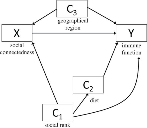
DAG showing the relationship between X and Y, and multiple confounders, C₁, C₂ and C₃.

While statistical adjustment is the most common approach to control for confounding, it can introduce bias in some instances due to use of an incorrect mathematical form of the covariate (e.g. entering a covariate as a continuous variable when it is not linearly associated with the outcome), heterogeneity of effects of X on Y across levels of the covariate (i.e. the existence of statistical interactions) and collinearity with other covariates. Thus, another option is inverse probability weighting (i.e. up-weighting or down-weighting the effect of a confounder based on its distribution in the study sample) to circumvent these issues [18–20]. Finally, there are other methods beyond the scope of this paper, such as use of instrumental variables (i.e. a proxy for X—often a gene or cluster of genes—that is strongly associated with X, affects Y through X only, and has no shared common causes with Y)—either alone or embedded in Rubin causal models [21]—that can capture an unbiased causal effect of X on Y.

(ii). Precision covariate

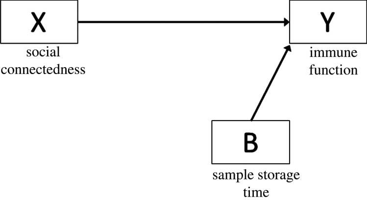
Precision covariates are associated with X only or Y only, denoted as B pointing towards X or Y (figure 5). Unlike confounders, there are no backdoor paths linking X to Y through B. Such variables account for technical variability and controlling for them in an analysis can improve model efficiency [22]. For instance, many analytes degrade over time, so biospecimen storage time is often included as a precision covariate in biomarker analyses.

Figure 5.

DAG showing the relationship between X and Y and precision covariate B.

(iii). Mediator

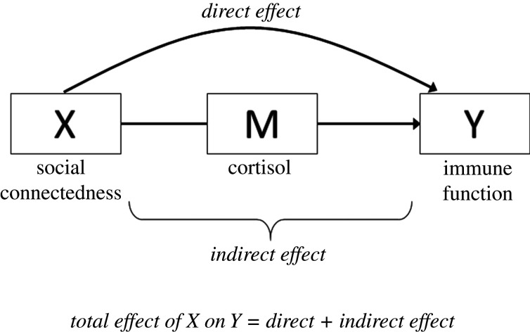
A researcher may be interested in the extent to which X affects Y after controlling for a variable M on the causal pathway between X and Y. As shown in figure 6, M is a consequence of X and a determinant of Y.

Figure 6.

DAG showing the relationship between X and Y, and mediator M.

Analyses that involve mediators are useful to assess mechanistic pathways linking X to Y. Say we suspect that chronic activation of hypothalamic–pituitary–adrenal (HPA) axis is a potential mechanism linking social connectedness to immune function [23]. This hypothesis may be tested using a regression-based approach after evaluating some assumptions: (i) the relationship between X and Y exists, (ii) M is associated with both X and Y, (iii) there is no interaction between X and M [24] and (iv) there are no common causes of M and Y other than X [25]. If the testable assumptions (i and ii above) are met, the analysis involves comparing the estimate for X before (total effect) versus after (direct effect) including M as a covariate in the model. If the estimate for X becomes attenuated after adjusting for M, then M might represent a mediating pathway.

This approach is widely used but limited in utility since violation of testable and non-testable assumptions can introduce major bias into the estimate of interest. The first assumption is that there should be no interaction between X and M. Empirically, this may be tested via a test for statistical interaction, but the determination of heterogeneity of effects still relies on arbitrary p-value thresholds for the X*M term. The second assumption is that there are no unmeasured confounders to M and Y, which cannot be tested empirically. In some instances, violation of this assumption can flip the direction of the estimate for X after conditioning on M. This is a form of collider bias [26], discussed later. The third assumption is that the variable M is a perfect proxy for the true mediator, which is rarely the case. In our example, cortisol is just one marker of HPA function that certainly does not capture the entire HPA cascade. Imperfect proxies for M lead to an underestimation of the mediating pathway (indirect effect) and an overestimation of the direct effect of X [22]. There are now a number of non-parametric methods that relax or circumvent some of these assumptions discussed elsewhere [5,27].

(iv). Effect modification

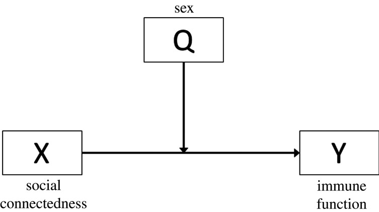
If we believe that the relationship between social connectedness and immune function differs with respect to an independent cause of Y, then our hypothesis involves effect modification. In our example, the same degree of social connectedness for males versus females may elicit differential effects on immune function [28,29]. An effect modifier (Q) changes the nature of the relationship between X and Y, or, in other words, introduces heterogeneity in the effect of X on Y across levels of Q [30] (figure 7).

Figure 7.

DAG showing the relationship between X and Y and effect modifier Q.

Effect modification may be assessed empirically via an interaction term between X and Q. If the p-value for the interaction term is significant, then effect modification is present. A parsimonious approach is to stratify the analyses by levels of Q if effect modification is suspected. While one may certainly interpret the estimate for the interaction term, this value only provides information on the difference in magnitude of the X → Y relationship for one level of Q relative to another. However, it does not tell you whether the direction of association differs for one level of Q versus another (e.g. males versus females in our example; see [31] for an in-depth discussion of qualitative versus quantitative interaction), which is biologically relevant. Importantly, keep in mind that unlike confounding, effect modification is an intrinsic phenomenon—a form of biological truth—that should be observed rather than ‘adjusted away'. The electronic supplementary material, §3 includes additional considerations for effect modification in the context of mediation analysis, along with a brief discussion on effect modification versus biological interaction.

(v). Collider

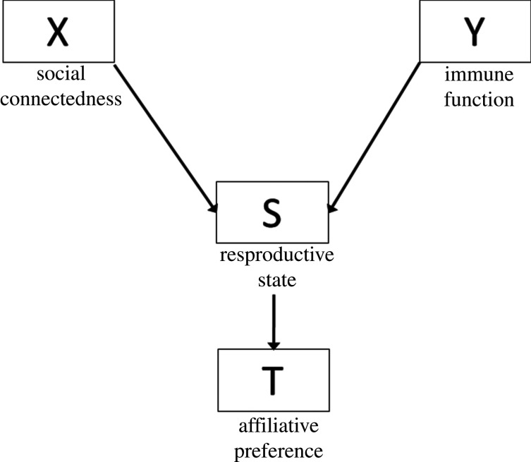
A collider (S) is a shared consequence of X and Y, depicted by arrows emerging from X and Y toward S. One should never condition on a collider, as this will induce a spurious association between X and Y.

If, as in figure 8, there is no association between X and Y, then conditioning on S (the collider) or T (consequence of the collider) will induce an association that does not exist. If an association does exist, conditioning on S can even flip the estimate for X in the opposite direction. In our example, reproductive state may be a collider since social connectedness can influence reproductive state (higher social connectedness is related to a greater likelihood of being pregnant) and immune function may also affect reproductive state (dysregulated immune function is associated failed pregnancy). In this scenario, conditioning on a reproductive state or affiliative preference forces us to consider associations between social connectedness and immune function only among those who are pregnant, and only among those who are not pregnant. If we adjust for the reproductive state in a regression model, the estimate for X is the average across the two levels of reproductive state (pregnant and non-pregnant). The strong positive association between social connectedness and immune function would skew the null association among those who are not pregnant to an overall positive association. This phenomenon is troubling and has puzzled perinatal epidemiologists who erroneously conditioned on the timing of parturition as a confounder when it was actually a collider [26].

Figure 8.

DAG showing the relationship between X and Y, collider S, and a consequence of the collider T.

Having encountered both confounders and colliders, we emphasize the utility of causal knowledge and DAGs to conceptualize both measured and unmeasured variables that may affect the relationship of interest, as opposed to relying solely on statistical associations [32,33].

(c) Step 3: implement the analysis

Prior to conducting the causal analysis that is reflected in the DAG(s), researchers should familiarize themselves with the data by assessing univariate and bivariate statistics (see electronic supplementary material, §2). There are typically two broad endpoints in a causal analysis: quantifying the total effect of X on Y and quantifying direct versus indirect effects (mediation) of X on Y.

(i). Total effects

If interested in the total effect of X on Y, the investigator should not adjust for mediators; doing so will yield null-biased estimates [22]. This does not imply that the investigator should avoid adjusting for confounders. As a shared common cause of X and Y, accounting for a confounder does not block any of the total effect of X but rather, controls for extraneous variability in the relationship between X and Y. Precision covariates should also be considered at this point in time.

After identifying confounders via a DAG and bivariate analysis, the next step is to home in on confounders to block all backdoor paths from X to Y. When the need to adjust for a variable is in question, we suggest examining the X → Y association with versus without adjustment for a variable. If including it does not appreciably change the results, then it is preferable to proceed without adjustment [22].

(ii). Direct and indirect effects

If a research question involves assessing a biological mechanism or pathway, then the analysis involves the estimation of direct and indirect effects. Barron and Kenny's method [24] is a common approach; however, as discussed earlier, there are limitations to this approach, and caution should be taken when interpreting results given the assumptions required and the fact that the variables for which we have data are likely upstream or downstream proxies of the true mediator or possibly markers of a parallel physiological pathway. Investigators should be particularly careful when testing mediators that cannot be directly manipulated, as these variables are particularly unlikely to meet the required assumptions [34]. In such scenarios, there are analytical techniques appropriate for mediation analysis, such as structural equations models and path analyses [35], which relax assumptions of generalized regression. Regardless, an investigator should not claim that the mechanism of interest is solely responsible for the effect of X on Y and acknowledge evidence from in vivo or in vitro studies and/or the need to interrogate specific mechanisms in controlled experimental settings.

(d). Step 4: interpret results

When interpreting the results, it is important to focus on the specific relationship between X and Y rather than for other covariates in the model. Moreover, the direction, magnitude and precision of the estimate across sensitivity analyses are important to assess since a robust association is likely to persist. Keep in mind that for any given hypothesis, there are alternate hypotheses and thus, alternate explanations for findings. Acknowledge and search for these possibilities, whether they transpire from complementary biological phenomena, unmeasured confounders or inappropriate statistical adjustment (e.g. adjusting baseline values of a variable when the outcome is changed in that variable [36,37], adjusting for a collider [38] or adjusting for a mediator that has a shared common cause with the outcome [26,39]). At this point in time, investigators may find it helpful to revisit the DAG after the analysis to sketch out unmeasured variables that may be responsible for surprising findings. Presenting the DAG and justifying the choice of variables and arrows therein is a valuable way of conveying the necessary assumptions that must hold for the results to be interpreted causally [40].

Finally, although there is stigma for using causal language to describe results from observational data, we and others [41] argue that use of causal language is appropriate when research tests a causal hypothesis and given appropriate consideration of alternative hypotheses and discussion biases.

4. Conclusion

Three years after pointing out the flaws of models, Box updated his outlook stating, ‘All models are wrong, but some are useful' [42]. In espousing Box's 1979 view, we hope that this commentary aids in developing useful models to answer impactful scientific questions, particularly when making a causal inference is the goal. For the interested reader who seeks to learn more about causal inference, we recommend starting with a layman's overview of causal inference in The Book of Why [41] and the freely available but somewhat more technical book, Causal Inference: What If [43].

Modern causal inference transpires from the work of torchbearers cited herein. Though many named epidemiologists may be unfamiliar to EEB scientists, Sewall Green Wright (1889–1988), an American evolutionary biologist known for his work involving path analysis, is a household name and a direct ancestor to modern causal inference [4,44]. Thus, while causal inference went out of fashion for much of the twentieth century among EEB researchers, it is rooted to luminaries in the field from the early to mid-nineteenth century. In recent years, a number of EEB scientists have developed an interest in causal inference and formed collaborations with epidemiologists and/or biostatisticians—a rich collaboration in which we hope to participate and promote.

Data accessibility

No empirical data were collected for this project.

Authors' contributions

Z.M.L. and W.P. conceived the ideas and led the writing of the manuscript; K.L.H. and R.J.S. provided content expertise relevant to behavioural ecology and evolutionary biology; and E.J.M. contributed expertise in causal inference. All authors contributed critically to the drafts and gave final approval for publication.

Competing interests

Authors declare no competing interests.

Funding

Z.M.L. is supported by the Morris Animal Foundation grant D19ZO-411. W.P. is supported by the Center for Clinical and Translational Sciences Institute KL2-TR002534. R.J.S. is supported by the National Science Foundation, IOS 1856266. K.L.H. is supported by National Science Foundation grant DEB-1911619.

References

- 1.Box GEP 1976. Science and statistics. J. Am. Stat. Assoc. 71, 791–799. ( 10.1080/01621459.1976.10480949) [DOI] [Google Scholar]
- 2.Tinbergen N 1963. On aims and methods of Ethology. Z Tierpsychol. 20, 410–433. [Google Scholar]
- 3.Shipley B 1999. Testing causal explanations in organismal biology: causation, correlation and structural equation modelling. Oikos. 86, 374–384. ( 10.2307/3546455) [DOI] [Google Scholar]
- 4.Wright S 1921. Correlation and causation. J. Agric. Res. 20, 557–585. [Google Scholar]
- 5.Zeng S, Rosenbaum S, Archie E, Alberts S, Li F. 2020. Causal mediation analysis for sparse and irregular longitudinal data. arXiv 27705.
- 6.Laubach ZM, et al. 2020. Associations of early social experience with offspring DNA methylation and later life stress phenotype. biorXiv.
- 7.Rosenbaum S, Zeng S, Campos FA, Gesquiere LR, Altmann J, Alberts SC, Li F, Archie EA. 2020. Social bonds do not mediate the relationship between early adversity and adult glucocorticoids inwild baboons. Proc. Natl Acad. Sci. USA 117, 20 052–20 062. ( 10.1073/pnas.2004524117) [DOI] [PMC free article] [PubMed] [Google Scholar]
- 8.Larsen AE, Meng K, Kendall BE. 2019. Causal analysis in control–impact ecological studies with observational data. Methods Ecol. Evol. 10, 924–934. ( 10.1111/2041-210X.13190) [DOI] [Google Scholar]
- 9.Hernán MA, Hsu J, Healy B. 2019. A second chance to get causal inference right: a classification of data science tasks. Chance 32, 42–49. ( 10.1080/09332480.2019.1579578) [DOI] [Google Scholar]
- 10.Conroy S, Murray EJ. 2020. Let the question determine the methods: descriptive epidemiology done right. Br. J. Cancer 123, 1351–1352. ( 10.1038/s41416-020-1019-z) [DOI] [PMC free article] [PubMed] [Google Scholar]
- 11.Albert JM, Cho JI, Liu Y, Nelson S. 2019. Generalized causal mediation and path analysis: extensions and practical considerations. Stat. Methods Med. Res. 28, 1793–1807. ( 10.1177/0962280218776483) [DOI] [PMC free article] [PubMed] [Google Scholar]
- 12.Mansournia MA, Altman DG. 2016. Inverse probability weighting. BMJ Res. Methods Rep. 352, 1–2. [DOI] [PubMed] [Google Scholar]
- 13.Naimi AI, Cole SR, Kennedy EH. 2017. An introduction to g methods. Int. J. Epidemiol. 46, 756–762. ( 10.1093/ije/dyx086) [DOI] [PMC free article] [PubMed] [Google Scholar]
- 14.Hernán MA 2016. Does water kill? A call for less casual causal inferences. Ann. Epidemiol. 26, 674–680. ( 10.1016/j.annepidem.2016.08.016) [DOI] [PMC free article] [PubMed] [Google Scholar]
- 15.Greenland S, Pearl J, Robins JM. 1999. Causal diagrams for epidemiologic research. Epidemiology 1, 37–48. ( 10.1097/00001648-199901000-00008) [DOI] [PubMed] [Google Scholar]
- 16.Sauer B, VanderWeele TJ. 2013. Use of directaed acyclic graphs. In Developing a protocol for observational comparative effectiveness research: A user's guide. AHRQ publi (eds Velentgas P, Dreyer NA, Smith SR, Torchia MM), pp. 177–184. Rockville, MD: Agency for Healthcare Research and Quality (AHRQ). [PubMed] [Google Scholar]
- 17.Greenland S, Pearl J, Robins JM. 1999. Causal diagrams for epidemiologic research. Epidemiology 10, 37–48. [PubMed] [Google Scholar]
- 18.Raad H, Cornelius V, Chan S, Williamson E, Cro S. 2020. An evaluation of inverse probability weighting using the propensity score for baseline covariate adjustment in smaller population randomised controlled trials with a continuous outcome. BMC Med. Res. Methodol. 20, 1–12. ( 10.1186/s12874-020-00947-7) [DOI] [PMC free article] [PubMed] [Google Scholar]
- 19.Ellis AR, Brookhart MA. 2013. Approaches to inverse-probability-of-treatment-weighted estimation with concurrent treatments. J. Clin. Epidemiol. 66(8 SUPPL.8), S51–S56. ( 10.1016/j.jclinepi.2013.03.020) [DOI] [PubMed] [Google Scholar]
- 20.Gruber S, Logan RW, Jarrín I, Monge S, Hernán MA. 2015. Ensemble learning of inverse probability weights for marginal structural modeling in large observational datasets. Stat. Med. 34, 106–117. ( 10.1002/sim.6322) [DOI] [PMC free article] [PubMed] [Google Scholar]
- 21.Angrist JD, Imbens GW, Rubin DB. 1996. Identification of causal effects using instrumental variables. J. Am. Stat. Assoc. 91, 444–455. ( 10.1080/01621459.1996.10476902) [DOI] [Google Scholar]
- 22.Schisterman EF, Cole SR, Platf RW. 2009. Overadjustment bias and unnecessary adjustment in epidemiologic studies. Epidemiology 20, 488–495. ( 10.1097/EDE.0b013e3181a819a1) [DOI] [PMC free article] [PubMed] [Google Scholar]
- 23.Segerstrom SC, Miller GE. 2004. Psychological stress and the human immune system: a meta-analytic study of 30 years of inquiry. Psychol. Bull. 130, 601–630. ( 10.1037/0033-2909.130.4.601) [DOI] [PMC free article] [PubMed] [Google Scholar]
- 24.Baron RM, Kenny DA. 1986. The moderator-mediator variable distinction in social psychological research: Conceptual, strategic, and statistical considerations. J. Pers. Soc. Psychol. 51, 1173–1182. ( 10.1037/0022-3514.51.6.1173) [DOI] [PubMed] [Google Scholar]
- 25.VanderWeele TJ 2015. Explanation in causal inference: methods for mediation and interaciton. New York, NY: Oxford University Press. [Google Scholar]
- 26.Ananth CV, Schisterman EF. 2017. Confounding, causality, and confusion: the role of intermediate variables in interpreting observational studies in obstetrics. Am. J. Obstet. Gynecol. 217, 167–175. ( 10.1016/j.ajog.2017.04.016) [DOI] [PMC free article] [PubMed] [Google Scholar]
- 27.Coffman DL, Zhong W. 2012. Assessing mediation using marginal structural models in the presence of confounding and moderation. Psychol. Methods 17, 642–664. ( 10.1037/a0029311) [DOI] [PMC free article] [PubMed] [Google Scholar]
- 28.Olsen NJ, Kovacs WJ. 1996. Gonadal steroids and immunity. Endocr Rev. 17, 369–384. [DOI] [PubMed] [Google Scholar]
- 29.Verthelyi D 2001. Sex hormones as immunomodulators in health and disease. Int. Immunopharmacol. 1, 983–993. ( 10.1016/S1567-5769(01)00044-3) [DOI] [PubMed] [Google Scholar]
- 30.VanderWeele TJ, Knol MJ. 2014. A tutorial on interaction. Epidemiol. Method 3, 33–72. [Google Scholar]
- 31.Szklo M, Nieto FJ. 2019. Epidemiology: beyond the basics, pp. 209–254. Sudbury, MA: Jones & Bartlett Publishers. [Google Scholar]
- 32.VanderWeele TJ, Robins JM. 2007. Directed acyclic graphs, sufficient causes, and the properties of conditioning on a common effect. Am. J. Epidemiol. 166, 1096–1104. ( 10.1093/aje/kwm179) [DOI] [PubMed] [Google Scholar]
- 33.Howards PP, Schisterman EF, Poole C, Kaufman JS, Weinberg CR. 2012. ‘Toward a clearer definition of confounding’ revisited with directed acyclic graphs. Am. J. Epidemiol. 176, 506–511. ( 10.1093/aje/kws127) [DOI] [PMC free article] [PubMed] [Google Scholar]
- 34.Murray EJ, Robins JM, Seage GR, Freedberg KA, Hernán MA. 2020. The challenges of parameterizing direct effects in individual-level simulation models. Med. Decis. Mak. 40, 106–111. ( 10.1177/0272989X19894940) [DOI] [PMC free article] [PubMed] [Google Scholar]
- 35.Edwards JR, Lambert LS. 2007. Methods for integrating moderation and mediation: a general analytical framework using moderated path analysis. Psychol. Methods. 12, 1–22. ( 10.1037/1082-989X.12.1.1) [DOI] [PubMed] [Google Scholar]
- 36.Glymour MM, Weuve J, Berkman LF, Kawachi I, Robins JM. 2005. When is baseline adjustment useful in analyses of change? An example with education and cognitive change. Am. J. Epidemiol. 162, 267–278. ( 10.1093/aje/kwi187) [DOI] [PubMed] [Google Scholar]
- 37.Pearl J 2014. Lord's paradox revisited—(Oh Lord! Kumbaya!). J. Causal Inference 4, 0021. [Google Scholar]
- 38.Hernán MA, Clayton D, Keiding N. 2011. The Simpson's paradox unraveled. Int. J. Epidemiol. 40, 780–785. ( 10.1093/ije/dyr041) [DOI] [PMC free article] [PubMed] [Google Scholar]
- 39.Tu YK, West R, Ellison GTH, Gilthorpe MS. 2005. Why evidence for the fetal origins of adult disease might be a statistical artifact: the ‘reversal paradox’ for the relation between birth weight and blood pressure in later life. Am. J. Epidemiol. 161, 27–32. ( 10.1093/aje/kwi002) [DOI] [PubMed] [Google Scholar]
- 40.Tennant PW, et al. 2019. Use of directed acyclic graphs (DAGs) in applied health research: review and recommendations. medRxiv.
- 41.Pearl J, Mackenzie D. 2018. The book of why: the new science of cause and effect. New York, NY: Basic Books. [Google Scholar]
- 42.Box GEP 1979. Robustness in the strategy of scientific model building. In Robustness in statistics (eds Launer RL, Wilkinson GN), pp. 201–236. New York, NY: Academic Press. [Google Scholar]
- 43.Hernán MA, Robins JM. 2020. Causal inference: what if. Boca Raton, FL: Chapman & Hall/CRC Taylor Francis Group. [Google Scholar]
- 44.Wright S 1960. Path coefficients and path regressions: alternative or complementary concepts? Biometrics 16, 189–202. ( 10.2307/2527551) [DOI] [Google Scholar]
Associated Data
This section collects any data citations, data availability statements, or supplementary materials included in this article.
Supplementary Materials
Data Availability Statement