Mathematical analysis of COVID-19 by using SIR model with convex incidence rate

Abstract

This paper is about a new COVID-19 SIR model containing three classes; Susceptible S(t), Infected I(t), and Recovered R(t) with the Convex incidence rate. Firstly, we present the subject model in the form of differential equations. Secondly, “the disease-free and endemic equilibrium” is calculated for the model. Also, the basic reproduction number $R_0$ is derived for the model. Furthermore, the Global Stability is calculated using the Lyapunov Function construction, while the Local Stability is determined using the Jacobian matrix. The numerical simulation is calculated using the Non-Standard Finite Difference (NFDS) scheme. In the numerical simulation, we prove our model using the data from Pakistan. “Simulation” means how S(t), I(t), and R(t) protection, exposure, and death rates affect people with the elapse of time.

Introduction

In December 2019, a new kind of virus named “corona” was reported to badly affect the Chinese city of Wuhan. The said virus and its resultant outbreak hit the city of Wuhan first and later affected almost the whole world. It took hundreds of thousands of lives worldwide. It is hard to take a single point of view on this virus’s origin. It may be due to a seafood market exchange, or the people’s migration from one place to another, or the transmission from animals to humans; It may also be due to human-to-human interactions. So far, the virus has devastated almost everything around the world. Social life, health, economy, education - generally, each segment of human life has been severely affected. Health researchers, governmental policymakers, and health care authorities are puzzled in combating the deadly outbreak. They all have their point of view on the situation. They are trying hard to, at least, minimize the number of deaths caused by the outbreak. The people infected in the coronavirus pandemic experience mild respiratory problems. Fever, dry cough, throat infection, and fatigue are the symptoms of this disease. People may also have the symptoms as follows; nasal infection, aches, and sore throat. Mathematical modeling plays an important role in describing the epidemic of infectious diseases. The purpose of mathematical modeling is to represent different types of a real-world situation in mathematical language. A number of mathematical model are studies in the pervious literature [1], [2], [8], [10]. Also SARS-CoV-2 is study by many researchers in current research literature [9], [11], [12], [14]. We will study SARS-CoV-2 by developing SEIR model later on in this work. Recently many authors have established numerious models for COVID-19 under different concept of fractional calculus. In this regards very useful models have been established, we refer some as [20], [21], [22], [23], [24], [25]. To find out the different dynamics of a disease and therefore to overcome it at an early stage, mathematical modeling plays an important role there [26], [27], [28]. The area dedicated to the investigation of biological pandemic and also epidemic models for recent diseases SARS-CoV-2 of research. Numerous examples of mathematical models for this pandemic are found in the current study [16], [17]. To understand the stability theory, existence theory, and theory of reform SARS-CoV-2 [6], [7], [13], [19], can be model, and its outcome can be predicted. Plan of prevention is also possible. In addition, one can find a possible lock-down strategy. Especially impressed with the excellent features of the SEIR model using non-linear saturated incidence rates [3], [4], [5], [6], [8], [15].

Model formulation

In this section of manuscript, we formulate our new model for $\mathit{NCOVID}-19$ in the form of following system (1). We take whole population N(t) into three classes S(t), I(t) and R(t), which represent Susceptible, Infected and Recovered compartment in the form of differential equations given below (1),

$$\begin{array}{c}\frac{\mathit{dS}(t)}{\mathit{dt}}=b-k(1-\alpha S(t)I(t))-\alpha k\beta S(t)I(t)-\mu S(t)\hfill \\ \frac{\mathit{dI}(t)}{\mathit{dt}}=k(1-\alpha S(t)I(t))+\alpha k\beta S(t)I(t)-(d_0+\gamma +\mu )I(t)\hfill \\ \frac{\mathit{dR}(t)}{\mathit{dt}}=\gamma I(t)-\mu R(t)\text{.}\hfill \end{array}$$ (1)

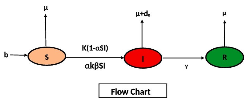
For above system (1) is presented in the form of flow chart as.

In Table 1 , we describe parameters used in system (1). In system (1), add all equations, implies

$$\frac{\mathit{dN}(t)}{\mathit{dt}}=-(\mu N(t)+d_{0}I(t)-b)\text{.}$$ (2)

Table 1.

Physical Interpretation of parameters of the system.

Parameters	The physical Description
$S(t)$	Susceptible compartment
$I(t)$	Infected compartment
$R(t)$	Recovered compartment
$d_0$	Death due to corona
$\mu$	Natural death
b	Birth rate
$\beta$	Protection rate
k	Constant rate
$\alpha$	Isolation rate
$\gamma$	Recovery rate

Here $N(t)$ represent whole population as $N(t)=S(t)+I(t)+R(t)$. We get

$$0⩽{\displaystyle \underset{t\to \infty }{\lim }}\mathit{supN}(t)⩽N_0\text{.}$$

With

$${\displaystyle \underset{t\to \infty }{\lim }}\mathit{supN}(t)=N_0\text{.}$$

If and only if

$${\displaystyle \underset{t\to \infty }{\lim }}\mathit{supI}(t)=0\text{.}$$

From the $1^{\mathit{st}}$ equation of the system (1), it show

$$0⩽{\displaystyle \underset{t\to \infty }{\lim }}\mathit{supS}(t)⩽S_0\text{.}$$

Which implies that if $N>N_0$, where $\frac{\mathit{dN}(t)}{\mathit{dt}}<0$. We can get

$$\mathrm{\Omega }=(S(t),I(t),R(t))\in {\mathbf{R}}_{+}^4:S(t)+I(t)+R(t)⩽N_0,S⩽S_0\text{.}$$

Equilibria

For the system (1), we suppose the existence of equilibrium. Disease free equilibrium is exist for some values of the variables used in (1), which is denoted by $E_0=(S^0,0,0)$.

$$E_0=(S^0,0,0)=\left(\frac{b}{\mu },0,0\right)\text{.}$$

Endemic equilibria

$$\begin{array}{c}{S}^{\ast }(t)=\frac{(\mu +d_0+\gamma )I^{\ast }(t)-b}{\mu }\hfill \\ I^{\ast }(t)=\frac{k\mu }{k\alpha (1-\beta )(\mu +d_0+\gamma -b)I^{\ast }(t)+\mu (\mu +d_0+\gamma )}\hfill \\ R^{\ast }(t)=\frac{\gamma }{\mu }{I}^{\ast }(t)\text{.}\hfill \end{array}$$

Expression for $R_0$ The basic reproductive number

In epidemiology there $R_0$ is most important parameter, which give us idea about how the disease is flow in the whole population. From $R_0$, we look how the disease id spread in population and we can control it from this. The method of finding $R_0$ is below let $X=(S(t),I(t))$, then from system (1),

$$\frac{\mathit{dX}}{\mathit{dt}}=\mathcal{F}-\mathcal{V},$$

where

$$\mathcal{F}=\left(\begin{array}{c}\hfill k(1-\alpha I(t)S(t))+\alpha k\beta I(t)S(t)\hfill \\ \hfill 0\hfill \end{array}\right)$$

and

$$\mathcal{V}=\left(\begin{array}{c}\hfill b-S(t)\hfill \\ \hfill (d_0+\gamma +\mu )I(t)\hfill \\ \hfill \hfill \end{array}\right)$$

Jacobian of $\mathcal{F}$ is

$$F=\left(\begin{array}{cc}\hfill -k\alpha S^0+k\alpha \beta S^0\hfill & \hfill 0\hfill \\ \hfill 0\hfill & \hfill 0\hfill \\ \hfill \hfill \end{array}\right)$$

and Jacobian of $\mathcal{V}$ is

$$V=\left(\begin{array}{cc}\hfill -\mu \hfill & \hfill 0\hfill \\ \hfill 0\hfill & \hfill d_0+\gamma +\mu \hfill \\ \hfill \hfill \end{array}\right)\text{.}$$

Hence

$$V^{-1}=\frac{1}{-\mu (\gamma +d_0+\mu )}\left(\begin{array}{cc}\hfill \mu +d_0+\gamma \hfill & \hfill 0\hfill \\ \hfill 0\hfill & \hfill -\mu \hfill \\ \hfill \hfill \end{array}\right)\text{.}$$

We have

$${\mathit{FV}}^{-1}=\left(\begin{array}{cc}\hfill k\alpha (\beta -1)S^0\hfill & \hfill 0\hfill \\ \hfill 0\hfill & \hfill 0\hfill \\ \hfill \hfill \end{array}\right)\text{.}$$

From this, we get $R_0$ is

$$R_0=\frac{k\alpha (1-\beta )b}{{\mu }^2}\text{.}$$ (3)

To computes the basic reproduction number we obtained $R_0=0.7831$ from the parameters used in Table 2 [18], which show that the COVID-19 that occurred in Pakistan is well controlled by Pakistan government. We have the following theorem on the basis of (3).

Theorem 1

(i) If$R_0\le 1$there is no positive equilibrium of system.

(ii) If$R_0>1$there is a unique positive equilibrium$E^{\ast }=(S^{\ast }(t),I^{\ast }(t),R^{\ast }(t))$of the model(1), called the endemic equilibrium.

Table 2.

Description of parameters and their values [18].

Parameters	Physical description	Numerical value
$S(t)$	Susceptible compartment	220 in millions
$I(t)$	Infected compartment	0 in million
$R(t)$	Recovered compartment	0 in million
$d_0$	Death due to corona	0.02
$\mu$	Natural death	0.0062
b	Birth rate	10.7
$\beta$	Protection rate	0.009, 0.0009
k	Constant rate	0.00761
$\alpha$	Isolation rate	0.009, 0.0009
$\gamma$	Recovery rate	0.0003

Local Stability

We reduced our model (1) for local stability. Furthermore, to obtained the result which show “disease free and endemic equilibrium”. For system (1). We reduced and get

$$\begin{array}{c}\frac{\mathit{dS}(t)}{\mathit{dt}}=b-k(1-\alpha S(t)I(t))-\alpha k\beta S(t)I(t)-\mu S(t)\hfill \\ \frac{\mathit{dI}(t)}{\mathit{dt}}=k(1-\alpha S(t)I(t))+\alpha k\beta S(t)I(t)-(\mu +d_0+\gamma )I(t)\text{.}\hfill \\ \hfill \end{array}$$ (4)

Subject to initial condition

$$S(0)=S_0⩾0,I(0)=I_0⩾0\text{.}$$

For local stability, we have the following theorem.

Theorem 2

If$R_0<1$, then the system(4)is locally asymptotically stable at the disease free equilibrium$E^0$.’

Proof

At $E^0$ the jacobian matrix is given by

$$J^0=\left(\begin{array}{cc}\hfill -\mu \hfill & \hfill \frac{k\alpha (1-\beta )b}{\mu }\hfill \\ \hfill 0\hfill & \hfill R_0-1\hfill \\ \hfill \hfill \end{array}\right)\text{.}$$

The auxiliary equation of $J^0$ is given by

$${\lambda }^3+{\lambda }^2{a}_1+\lambda a_2+a_3=0,$$

where

$$\begin{array}{cc}\hfill & a_1=(\mu +\beta )(\mu +\alpha )+(\mu +d_0+\gamma )(1-R_0)>0\hfill \\ \hfill & a_2=(\mu +\beta )(\mu +\beta )[1+(\mu +\gamma +d_0)(1-R_0)]>0\hfill \\ \hfill & a_3=(\mu +\beta )(\mu +\alpha )(\mu +\gamma +d_0)(1-R_0)>0\text{.}\hfill \end{array}$$

We have

$$a_1{a}_2-a_3=(\mu +\beta )(\mu +\alpha )\left({(\mu +\gamma +d_0)}^2+(\mu +\beta )(\mu +\alpha )[(d_0+\gamma +\mu )+1]\right)\left(1-R_0\right)>0\text{.}$$ (5)

The Routh-Hurtwriz criteria is satisfied as $a_1>0,a_2>0,a_3>0$ and $a_1{r}_2-r_3>0$ if $R_0<1$. which show the system (1) is locally asymptotically stable at $E^0$.

Furthermore, at $E^{\ast }$ the system (4) is locally asymptotically stability analogous to $R^0>1$. We are going to prove it in the next theorem.

Theorem 3

At$E^{\ast }$, if$R^0>1$then system(4)is locally asymptotically stable.

Proof

For system (4) jacobian matrix is

$$J_1=\left(\begin{array}{cc}\hfill \alpha {\mathit{kI}}^{\ast }(t)-\mu -\alpha k\beta I^{\ast }(t)\hfill & \hfill \alpha {\mathit{kS}}^{\ast }(t)-\alpha k\beta S^{\ast }(t)\hfill \\ \hfill -\alpha {\mathit{kI}}^{\ast }(t)+\alpha k\beta I^{\ast }(t)\hfill & \hfill -k\alpha S^{\ast }(t)+\alpha k\beta S^{\ast }(t)-(\mu +d_0+\gamma )\hfill \\ \hfill \hfill \end{array}\right)\text{.}$$

After some operations on matrix $J_1$, we get

$$M_1=\left(\begin{array}{cc}\hfill -\mu \hfill & \hfill -(\mu +d_0+\gamma )\hfill \\ \hfill -\alpha k(1-\beta )I^{\ast }(t)\hfill & \hfill -k\alpha (1+\beta )S^{\ast }(t)-(\mu +d_0+\gamma )\hfill \\ \hfill \hfill \end{array}\right)\text{.}$$

We calculate trace and determinant of $M_1$

$$\mathit{tra}(M_1)=-2\mu -k\alpha (\beta +1)S^{\ast }(t)-d_0-\gamma <0,$$ (6)

and

$$\det (M_1)=\mu \left[\alpha \beta (1+\beta )+d_0+\mu +\gamma \right]+\alpha k(\mu +d_0+\gamma )(\beta +1)>0\text{.}$$ (7)

The determinant of $J_1>0$. The real part at $E^{\ast }(t)$ “endemic equilibrium” of model (4) has negative. Thus, with condition $R_0>1$, we have that the endemic equilibrium $E^{\ast }$ of system (4) is locally asymptotically stable.

Global stability

Here, we present Global stability for the system (1). For “global stability of disease-free and endemic equilibrium”, we constructed a function known as Lyapunov function in the following theorem.

Theorem 4

If$R_0<1$then disease free equilibrium of the system(4)is globally asymptotically stable. Otherwise unstable.

Proof

To prove this, we construct a Lyapunov function as following

$$\rho =c_1(S(t)-S_0)+c_{3}I(t),$$ (8)

such that $c_1,c_2,c_3>0$ are constants. With respect to time t taking derivative of (8) with, we have

$$\frac{d\rho }{\mathit{dt}}=c_1\left(b-k(1-\alpha S(t)I(t))b-\alpha k\beta S(t)I(t)-\mu S(t)\right)+c_2(k(1-\alpha S(t)I(t))+\alpha k\beta S(t)I(t)-(\mu +d_0+\gamma )I(t))\text{.}$$

We get

$$\frac{d\rho }{\mathit{dt}}=c_{1}b+k(1-\alpha S(t)I(t))(c_2-c_1)+\alpha k\beta S(t)I(t)(c_2-c_1)+c_1\mu S(t)-c_2\mu I(t)-c_1{d}_{0}I(t)-c_2\gamma I(t)\text{.}$$

Let assume $c_1=c_2=c_3=1$, we get finally

$$\frac{d\rho }{\mathit{dt}}=-(\mu N(t)-b)-(d_0+\gamma )I(t)<0\text{.}$$

Hence “globally asymptotically stable” for system (1) with $R_0<1$ has reached. Further, We are going to prove a theorem for “global stability of the endemic equilibrium” of model (1).

Theorem 5

The endemic equilibrium$E^{\ast }$of model(1)is stable globally asymptotically if$R_0>1$.

Proof

By constructing Lyapunov function, we prove the above result

$$\omega =(\mu +\beta )(S(t)-S^{\ast }(t))+(\mu +\beta )I(t)\text{.}$$ (9)

Taking derivative with respect to time (9), we get

$$\frac{d\omega }{\mathit{dt}}=(\mu +\beta )S^{.}(t)+(\mu +\beta )I^{.}(t)\text{.}$$

Putting the values from (1)

$$\frac{d\omega }{\mathit{dt}}=(\mu +\beta )(b-k(1-\alpha S(t)I(t))-\alpha k\beta S(t)I(t)-\mu S(t))+(\mu +\beta )(k(1-\alpha S(t)I(t))+\alpha k\beta S(t)I(t)-(\mu +d_0+\gamma )I^{\ast }(t))\text{.}$$

After some arrangement we get

$$\frac{d\omega }{\mathit{dt}}=-(\mu +\beta )(\mu S(t)+(\mu +d_0+\gamma )I^{\ast }(t))<0\text{.}$$

Thus $\frac{d\omega }{\mathit{dt}}<0$, the “endemic equilibrium” $E^{\ast }$ of the model (1) is “ globally asymptotically stable”, show that $R_0>1$.

Numerical results and discussion

In this part of our manuscript, we calculated numerical simulation for model (1) with values used on Table 2. We take data from 1 February 2020 to $20\mathit{th}$ September corresponding to different compartments involve in the system (1) from Pakistan. Here, we use (NSFD) Non-standard Finite Difference scheme [13], [15], [19] to rewrite the system is

$$\frac{\mathit{dS}(t)}{\mathit{dt}}=b-k(1-\alpha S(t)I(t))-\alpha k\beta S(t)I(t)-\mu S(t)\text{.}$$ (10)

Which is decomposed in Nonstandard Finite Difference scheme as

$$\frac{S_{j+1}-S_j}{h}=b-k(1-\alpha S_j(t)I_j(t))-\alpha k\beta S_j(t)I_j(t)-\mu S_j(t)\text{.}$$ (11)

Just like above Eq. (11), we can write the system (1) in Non-Standard Finite Difference Scheme as

$$\begin{array}{cc}\hfill & S_{j+1}=S_j+h\left(b-k(1-\alpha S_j(t)I_j(t))-\alpha k\beta S_j(t)I_j(t)-\mu S_j(t)\right)\hfill \\ \hfill & I_{j+1}=I_j+h\left(k(1-\alpha S_j(t)I_j(t))+\alpha k\beta S_j(t)I_j(t)-(d_0+\gamma +\mu )I_j(t)\right)\hfill \\ \hfill & R_{j+1}=R_j+h\left(\gamma I_j(t)-\mu R_j(t)\right)\text{.}\hfill \end{array}$$ (12)

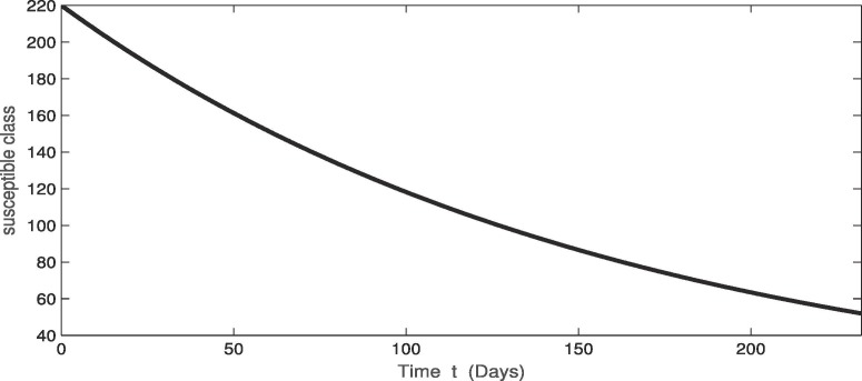
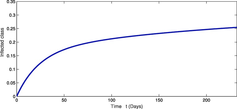
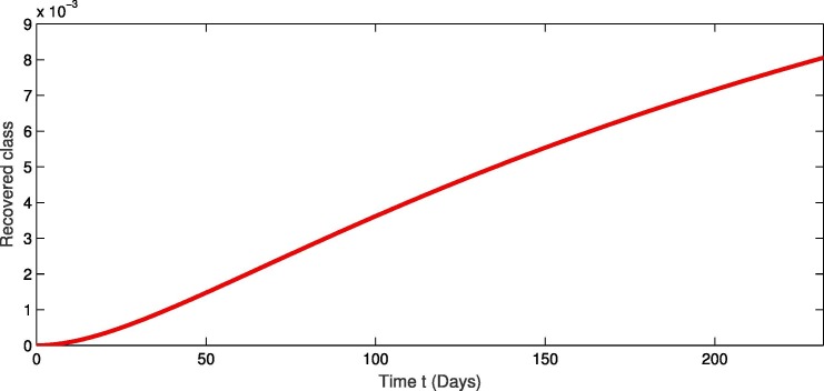
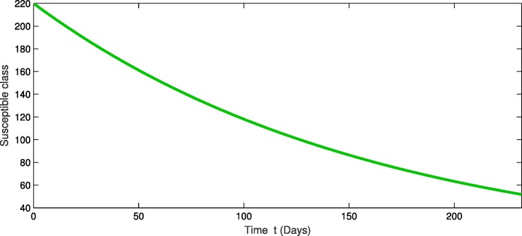
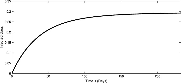
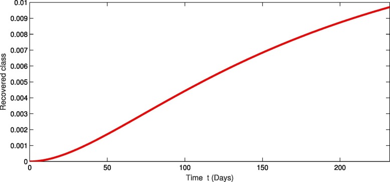
For the real data of Pakistan [18], we testified our model (1) taking the values of parameter of Table 2 from first February 2020 to 20th of September 2020. From Fig. 1, Fig. 2, Fig. 3 , we see that as the susceptibility was decreasing the infection was increasing in first four months but in the month of July and August the infection rate became slow and finally in the last it was nearly become stable. Also during this time the recovery rate was rapid from the infection as in Fig. 3. The concerned simulation was performed for taking the protection parameter $\alpha =\beta =0.009$. Now by deceasing the protection and isolation rate further up to $\alpha =0.0009,\beta =0.0009$. We plot the results in the given Fig. 4, Fig. 5, Fig. 6 . We see that the infection rate became slow on reducing the protection and isolation rate. Therefore the recovery is also become slow. From these simulation we observed that protection and isolation rate play significant roles in controlling the infection from further spreading in the community. see Fig. 2,.

Fig. 1.

Dynamical behavior in of susceptible population of the considered model.

Fig. 2.

Dynamical behavior of infected population of the considered model.

Fig. 3.

Dynamical behavior of recovered population of the considered model.

Fig. 4.

Dynamical behavior in of susceptible population of the considered model.

Fig. 5.

Dynamical behavior of infected population of the considered model.

Fig. 6.

Dynamical behavior of recovered population of the considered model.

Conclusion

Conclusion of the numerical results shows the projection of model (1). The output derived from the NCOVID-19 display convex incidence rate. The current manuscript declared the high contiguous rate from infected population to susceptible population. To overcome the pandemic the migration should be strictly prohibited for the sake of saving humanity. Also the immigration of exposed population to infected community increased the infection. Isolation of infected one is the best option to secured the healthy community. It is necessary to judge the spread and model with various parameters for proper supervision. The proper treatment of this pandemic is to keep infected away from healthy people. High internal defense system aids to get healthy soon while the low internal defense system need more attention. This is the only solution to overcome recent outbreak within a short period. The current discussion demonstrate the quick transfer of NCOVID-19. The COVID-19 shared the same properties like SARS having mortality rate of 2 percent. There is no vaccine available in the current time but to isolate was the best option. Also social distancing is the best way to control this deadly various.

Funding

There is no source to support this article financially.

Availability of Data

This is not applicable in this research work.

Declaration of Competing Interest

The authors declare that they have no known competing financial interests or personal relationships that could have appeared to influence the work reported in this paper.

References

- 1.World Health Organization (WHO), Naming the coronavirus disease (COVID-19)) and the virus that causes it, Archived from the original on 28 February 2020. Retrieved 28 February, (2020).
- 2.Hui DSI, Azhar E. Madani, T.A. Ntoumi, F. Kock, R. Dar, O. Ippolito, G. Mchugh, T.D. Memish, Z.A. Drosten, Christian, Zumla, A.; Petersen, E, The continuing 2019-nCoV epidemic threat of novel coronaviruses to global health-The latest 2019 novel coronavirus outbreak in Wuhan, China, Bulletin of Mathematical Biology, 91(6) (2020) 264-66. [DOI] [PMC free article] [PubMed]
- 3.Zhao S., Lin Q., Ran J., Musa S.S., Yang G., Wang W., et al. Preliminary estimation of the basic reproduction number of novel coronavirus (2019-nCoV) in China. Int J Infectious Diseases. 2020;92:214–217. doi: 10.1016/j.ijid.2020.01.050. [DOI] [PMC free article] [PubMed] [Google Scholar]
- 4.Zhao S., Musa S.S., Lin Q., Ran J., Yang G., Wang W., Lou Y., Yang L., Gao D., He D., Wang M.H. Estimating the unreported number of novel coronavirus (2019-nCoV) cases in China in the first half of January 2020, a data-driven Modelling analysis of the early outbreak. J Clin Med. 2020;9(2):388. doi: 10.3390/jcm9020388. [DOI] [PMC free article] [PubMed] [Google Scholar]
- 5.Nesteruk I. Statistics based predictions of coronavirus 2019-nCoV spreading in mainland China. MedRxiv. 2020;4(1):1988–1989. [Google Scholar]
- 6.Ming W.K., Huang J., Zhang C.J. Breaking down of healthcare system: Mathematical modelling for controlling the novel coronavirus (2019-nCoV) outbreak in Wuhan, China. bioRxiv. 2020 [Google Scholar]
- 7.Lotka Alfred J. Contribution to the theory of periodic reactions. J Phys Chem. 2002;14(3):271–274. [Google Scholar]
- 8.Goel Narendra S., Maitra Samaresh C., Montroll Elliott W. On the Volterra and other nonlinear models of interacting populations. Rev Modern Phys. 1971;43(2):231. [Google Scholar]
- 9.Zhou P., Yang X.L., Wang X.G., Hu B., Zhang L., Zhang W., Si H.R., Zhu Y., Li B., Huang C.L., Chen H.D. A pneumonia outbreak associated with a new coronavirus of probable bat origin. nature. 2020;579(7798):270–273. doi: 10.1038/s41586-020-2012-7. [DOI] [PMC free article] [PubMed] [Google Scholar]
- 10.Li, Qun and Guan, Xuhua and Wu, Peng and Wang, Xiaoye and Zhou, Lei and Tong, Yeqing and Ren, Ruiqi and Leung, Kathy SM and Lau, Eric HY and Wong, Jessica Y and others, Early transmission dynamics in Wuhan, China, of novel coronavirus infected pneumonia, New England Journal of Medicine, 382 (2020) 1199–1207. [DOI] [PMC free article] [PubMed]
- 11.Bogoch I.I., Watts A., Thomas-Bachli A., Huber C., Kraemer M.U., Khan K. Pneumonia of unknown aetiology in Wuhan, China: potential for international spread via commercial air travel. J Travel Med. 2020;27(2):taaa008. doi: 10.1093/jtm/taaa008. [DOI] [PMC free article] [PubMed] [Google Scholar]
- 12.Gumel A.B., et al. Modelling strategies for controlling SARS out breaks. Proc R Soc Lond B. 2004;271(1554):2223–2232. doi: 10.1098/rspb.2004.2800. [DOI] [PMC free article] [PubMed] [Google Scholar]
- 13.Algehyne E.A., ud Din R. On global dynamics of COVID-19 by using SQIR type model under non-linear saturated incidence rate. Alexandria Eng J. 2020;60(1):393–399. [Google Scholar]
- 14.Wu J.T., Leung K., Leung G.M. Nowcasting and forecasting the potential domestic and international spread of the 2019-nCoV outbreak originating in Wuhan, China: a modelling study. Lancet. 2020;395(10225):689–697. doi: 10.1016/S0140-6736(20)30260-9. [DOI] [PMC free article] [PubMed] [Google Scholar]
- 15.Rahman G., et al. Host vector dynamics of pine wilt disease model with convex incidence rate. Chaos, Solitons Fractals. 2018;113:31–39. [Google Scholar]
- 16.Kanagarathinam Karthick, Algehyne Ebrahem A., Sekar Kavaskar. Analysis of ‘earlyR’ epidemic model and time series model for prediction of COVID-19 registered cases. Materials Today: Proc. 2020 doi: 10.1016/j.matpr.2020.10.086. [DOI] [PMC free article] [PubMed] [Google Scholar]
- 17.Muhammad L.J., Algehyne E.A., Usman S.S., Ahmad A., Chakraborty C., Mohammed I.A. Supervised Machine Learning Models for Prediction of COVID-19 Infection using Epidemiology Dataset. C SN Computer Sci. 2021;2(1):1–13. doi: 10.1007/s42979-020-00394-7. [DOI] [PMC free article] [PubMed] [Google Scholar]
- 18.https://www.worldometers.info/coronavirus/country/pakistan, 2 February to 20 September, 2021.
- 19.Peter M. Manning and Gary F. Margrave, Introduction to non-standard finite-difference modelling, CREWES Research Report, 18 (2006) 10 page.
- 20.Khan M.A., Atangana A. Modeling the dynamics of novel coronavirus (2019-nCov) with fractional derivative. Alexandria Eng J. 2020;59(4):2379–2389. [Google Scholar]
- 21.Khan M.A., Atangana A., Alzahrani E. The dynamics of COVID-19 with quarantined and isolation. Adv Diff Eq. 2020;2020(1):1–22. doi: 10.1186/s13662-020-02882-9. [DOI] [PMC free article] [PubMed] [Google Scholar]
- 22.Boccaletti S., Ditto W., Mindlin G., Atangana A. Modeling and forecasting of epidemic spreading: The case of Covid-19 and beyond. Chaos, Solitons, Fractals. 2020;135 doi: 10.1016/j.chaos.2020.109794. [DOI] [PMC free article] [PubMed] [Google Scholar]
- 23.Atangana E., Atangana A. Facemasks simple but powerful weapons to protect against COVID-19 spread: Can they have sides effects? Results Phys. 2020;19 doi: 10.1016/j.rinp.2020.103425. [DOI] [PMC free article] [PubMed] [Google Scholar]
- 24.Thabet S.T., Abdo M.S., Shah K., Abdeljawad T. Study of transmission dynamics of COVID-19 mathematical model under ABC fractional order derivative. Results Phys. 2020;19 doi: 10.1016/j.rinp.2020.103507. [DOI] [PMC free article] [PubMed] [Google Scholar]
- 25.Boccaletti S., William D., Mindlin G., Atangana A. Modeling and forecasting of epidemic spreading: The case of Covid-19 and beyond. Chaos, Solitons, Fractals. 2020;135 doi: 10.1016/j.chaos.2020.109794. [DOI] [PMC free article] [PubMed] [Google Scholar]
- 26.Kanagarathinam Karthick, Ebrahem A. Algehyne, Kavaskar Sekar Analysis of ‘earlyR’ epidemic model and time series model for prediction of COVID-19 registered cases. Materials Today: Proceedings. 14 Oct 2020 doi: 10.1016/j.matpr.2020.10.086. [DOI] [PMC free article] [PubMed] [Google Scholar]
- 27.L. Muhammad, J., Algehyne Ebrahem, A., et al. Supervised Machine Learning Models for Prediction of COVID‑19 Infection using Epidemiology Dataset. SN Computer Science. 2020;2(11) doi: 10.1007/s42979-020-00394-7. [DOI] [PMC free article] [PubMed] [Google Scholar]
- 28.L. Muhammad, J., Algehyne Ebrahem., A. Fuzzy based expert system for diagnosis of coronary artery disease in nigeria. Health and Technology. 2021 doi: 10.1007/s12553-021-00531-z. [DOI] [PMC free article] [PubMed] [Google Scholar]
Associated Data
This section collects any data citations, data availability statements, or supplementary materials included in this article.
Data Availability Statement