Mathematical analysis of a stochastic model for spread of Coronavirus

Abstract

This paper is associated to investigate a stochastic SEIAQHR model for transmission of Coronavirus disease 2019 that is a recent great crisis in numerous societies. This stochastic pandemic model is established due to several safety protocols, for instance social-distancing, mask and quarantine. Three white noises are added to three of the main parameters of the system to represent the impact of randomness in the environment on the considered model. Also, the unique solvability of the presented stochastic model is proved. Moreover, a collocation approach based on the Legendre polynomials is presented to obtain the numerical solution of this system. Finally, some simulations are provided to survey the obtained results of this pandemic model and to identify the theoretical findings.

1. Introduction

Using dynamical systems to describe behaviors of infectious diseases is an effective way to study how these diseases spread [1], [2], [3]. Mathematical models can greatly help researchers to better understand behaviors of deadly diseases around the world. The Susceptible-Infectious-Recovered (SIR) approach is a well-known basic model to analyze and to predict the epidemic of contagious diseases. Many researchers employed theoretical frameworks and numerical simulations to survey the manner of transmission of different infectious diseases [4], [5], [6], [7], [8], [9], [10], [11], [12], [13].

In recent months, a specific group of viruses, named Coronavirus, has disrupted life around the world. Coronaviruses have a “crown” or corona of sugary-proteins. Thus, they have named Coronaviruses according to their specific appearance, in 1960. Special cases of Coronaviruses are the main sources of certain popular diseases such as the Middle East respiratory syndrome (MERS-CoV) and severe acute respiratory syndrome (SARS-CoV). Researches have shown that these viruses are conveyed between humans and animals. For example, MERS-CoV and SARS-CoV have transmitted from dromedary camels and civets to humans, respectively. Some Coronavirus strains are only active in animals and have not yet infected human beings.

The Wuhan city in China was the first place that the Coronavirus disease 2019 (COVID-19) was identified. This new version of Coronaviruses was not previously diagnosed in human beings. Experts refer to different sources for this disease. Some of them believe the virus was first transmitted from pangolins or bats to humans in China. The high rate of contagion has caused that countries all over the world are affected by COVID-19. Cough, fever, difficulties in breathing and loss of sense of taste and smell are the main signs of the disease. High mortality rate and the serious economic and financial crisis created by the Coronavirus pandemic have motivated many researchers to study the behaviors of this virus and to find effective ways for facing this outbreak. Hence, some suitable susceptible-exposed-infectious-recovered (SEIR) type models are presented in these investigations to simulate the dynamic of the COVID-19 pandemic. The impact of asymptomatic category and quarantine on the transmission of COVID-19 [14], modeling the COVID-19 due to the interactivity between the animals, humans and the infections reservoir such as seafood market [15], investigating the dynamics of COVID-19 epidemics using real data from Pakistan [16], a model for the transmission of COVID-19 based on the Caputo-Fabrizio fractional order derivative [17], a stochastic model to study the stationary distribution and extinction of coronavirus epidemic [18], a stochastic model to evaluate healthcare impact of Coronavirus in India [19], modeling the potential for mask use to curtail the COVID-19 [20], using fuzzy neural network models to predict COVID-19 time series in Mexico [21], investigation about the role of non-pharmaceutical interventions on reducing COVID-19 [22] and identifying the effect of social distancing in diminishing COVID-19 in Canada [23] are some examples of these scientific works.

In this work, first, we suggest a deterministic model to analyze the impact of preventive and health-protective measures such as quarantine, using masks and social distancing on the Coronavirus prevalence. A parameter called the force of infection is considered in the model. This parameter is affected by the factors related to the mentioned safety health protocols. Thus, this novel biological parameter helps us to verify the impact of safety strategies on the control of the disease. Many relationships between people are based on random contacts. So, by considering random parameters in the proposed deterministic model, a more realistic stochastic model for COVID-19 will be derived. Also, a new high-order numerical technique is introduced to find more accurate and reliable results for the presented biological system.

This paper has the following organization. In Section 2, a deterministic model for COVID-19 is presented based on some general strategies. Also, the analysis of this deterministic model will be developed. A stochastic model for the spread of Coronavirus is discussed in Section 3 and the existence of a unique positive solution for this system will be proved. In Section 4, a step-by-step collocation scheme is introduced and in Section 5, this method is employed to provide numerical simulations of the proposed stochastic model. At the end, the main conclusions are presented in Section 6.

2. The deterministic COVID-19 model

In the rest, the supposed population will be divided into several compartments to adapt a SEIR-type model describing the evolution of the COVID-19 pandemic. For simulation, the total size of the population under study is supposed to equal to $\mathrm{N}\left(t\right)$.

In the survey conducted, every individual belongs to one of the following seven categories:

• $⧫$ the class $\mathrm{S}$ includes susceptible individuals who never infected before;

• $⧫$ the class $\mathrm{E}$ includes the individuals that have been newly-infected but those are not still sick and cannot transmit infection;

• $⧫$ the class $\mathrm{I}$ includes the infectious individuals with symptoms;

• $⧫$ the class $\mathrm{A}$ includes the infectious individuals that are not yet symptoms;

• $⧫$ the class $\mathrm{Q}$ includes the infectious individuals that are with slight symptoms and hence are at home quarantine;

• $⧫$ the class $\mathrm{H}$ includes the infectious individuals that are hospitalized;

• $⧫$ the class $\mathrm{R}$ includes the recovered individuals from the disease;

where

$$\mathrm{N}\left(t\right)=\mathrm{S}\left(t\right)+\mathrm{E}\left(t\right)+\mathrm{I}\left(t\right)+\mathrm{A}\left(t\right)+\mathrm{Q}\left(t\right)+\mathrm{H}\left(t\right)+\mathrm{R}\left(t\right).$$

Now, to introduce our model, we need to define some parameters. Let $c$ and $\theta$ show the contact and the transmission rates, respectively. $q$ represents the rate of quarantine for exposed persons. $\Lambda$ is the birth rate. To consider the effectiveness of social-distancing, the effective contact rate $\beta$ is defined. ${\delta }_{\mathrm{I}}$ displays the transition rate from the symptomatic infected category to the quarantined infected category. ${\gamma }_{\mathrm{I}}$ and ${\gamma }_{\mathrm{A}}$ are the recovery rates of symptomatic infected persons and asymptomatic infected persons, respectively and ${\gamma }_{\mathrm{H}}$ is the recovery rate of individuals in the class $\mathrm{H}$. Also, ${\alpha }_{\mathrm{A}}$ and ${\alpha }_{\mathrm{I}}$ show the movement rate from the class $\mathrm{Q}$ to the class $\mathrm{A}$ and the transition rate from $\mathrm{A}$ to the class $\mathrm{I},$ respectively. $\rho$ and ${\mu }_{\mathrm{I}}$ represent the symptoms rate among infected individuals and the mortality rate due to Coronavirus, respectively. Moreover, $c_m$ is the proportion of people who use masks and ${\epsilon }_m$ represents the effect of using mask to prevent catching the infection by susceptible individuals. $0\le {\theta }_q\le 1$ is the efficacy of quarantine and hospitalization admission in preventing virus transmission. Finally, $\phi ,$ $\overline{\rho }$ and $\mu$ represent the proportion of infected individuals with symptoms in quarantine, the movement rate from the category $\mathrm{Q}$ to $\mathrm{I}$ and the natural death rate, respectively. Let, the force of infection, $\lambda ,$ be defined as:

$$\lambda =\beta (1-{\epsilon }_m{c}_m)\frac{\mathrm{I}+\theta \mathrm{A}}{\mathrm{N}-{\theta }_q(\mathrm{Q}+\mathrm{H})}.$$ (1)

Then, according to the above variables and parameters, we have the following proposed system of equations for the dynamics of COVID-19:

$$\{\begin{array}{c}\dot{\mathrm{S}}=\Lambda -(\lambda +\mu )\mathrm{S},\hfill \\ \dot{\mathrm{E}}=\lambda \mathrm{S}-(c+\mu )\mathrm{E},\hfill \\ \dot{\mathrm{I}}=c\rho (1-q)\mathrm{E}+\phi \overline{\rho }\mathrm{Q}+{\alpha }_{\mathrm{I}}\mathrm{A}-({\gamma }_{\mathrm{I}}+{\delta }_{\mathrm{I}}+{\mu }_{\mathrm{I}}+\mu )\mathrm{I},\hfill \\ \dot{\mathrm{A}}=c(1-\rho )(1-q)\mathrm{E}+{\alpha }_{\mathrm{A}}\mathrm{Q}-({\alpha }_{\mathrm{I}}+{\gamma }_{\mathrm{A}}+\mu )\mathrm{A},\hfill \\ \dot{\mathrm{Q}}=cq\mathrm{E}-({\alpha }_{\mathrm{A}}+\phi \overline{\rho }+\mu )\mathrm{Q},\hfill \\ \dot{\mathrm{H}}={\delta }_{\mathrm{I}}\mathrm{I}-({\gamma }_{\mathrm{H}}+{\mu }_{\mathrm{I}}+\mu )\mathrm{H},\hfill \\ \dot{\mathrm{R}}={\gamma }_{\mathrm{I}}\mathrm{I}+{\gamma }_{\mathrm{A}}\mathrm{A}+{\gamma }_{\mathrm{H}}\mathrm{H}-\mu \mathrm{R}.\hfill \end{array}$$ (2)

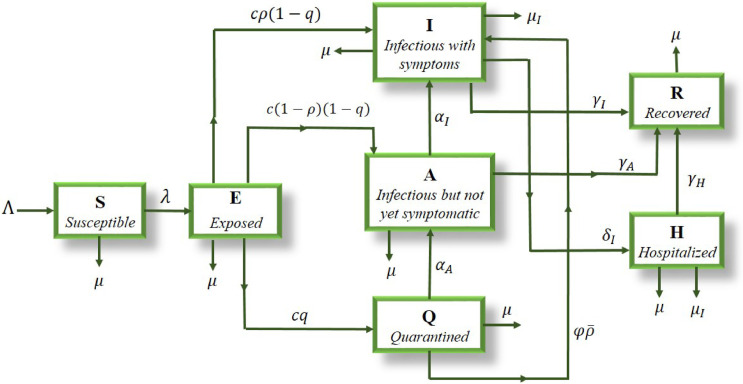
The diagram of this model is illustrated in Fig. 1 .

Fig. 1.

The diagram of the proposed coronavirus transmission model.

The disease free equilibrium point of the model (2) can be obtained as

$${\mathcal{E}}^0={(\frac{\Lambda }{\mu },0,0,0,0,0,0)}^{\mathrm{T}}.$$ (3)

To assess the transmissibility of the disease, it is needed to get the basic reproduction number ${\mathcal{R}}_0,$ i.e. the expected number of new infections that result from a single infectious person in a specific population of susceptible individuals. To determine this number for the COVID-19 model (2), we employ the method proposed in [24]. Suppose $\varpi :=\beta (1-{\epsilon }_m{c}_m)$. The matrix of new infection terms $\mathcal{F}$ and the matrix of the remaining transmission terms $\mathcal{V}$ for the model (2) are defined as $\mathcal{F}\left({\mathcal{E}}^0\right)={\left[{\mathbf{f}}_{i,j}\right]}_{5\times 5}$ where

$${\mathbf{f}}_{i,j}=\{\begin{array}{c}\varpi ,i=1,j=2,\hfill \\ \theta \varpi ,i=1,j=3,\hfill \\ 0,o.w.,\hfill \end{array}$$

and

$$\mathcal{V}\left({\mathcal{E}}^0\right)=\left(\begin{array}{ccccc}{\varsigma }_1\hfill & 0\hfill & 0\hfill & 0\hfill & 0\hfill \\ {\varsigma }_2\hfill & {\varsigma }_3\hfill & {\varsigma }_4\hfill & {\varsigma }_5\hfill & 0\hfill \\ {\varsigma }_6\hfill & 0\hfill & {\varsigma }_7\hfill & {\varsigma }_8\hfill & 0\hfill \\ {\varsigma }_9\hfill & 0\hfill & 0\hfill & {\varsigma }_{10}\hfill & 0\hfill \\ 0\hfill & {\varsigma }_{11}\hfill & 0\hfill & 0\hfill & {\varsigma }_{12}\hfill \end{array}\right),$$

in which

$$\begin{array}{cccc}{\varsigma }_1:=c+\mu ,\hfill & {\varsigma }_2:=-c\rho (1-q),\hfill & {\varsigma }_3:={\delta }_{\mathrm{I}}+{\gamma }_{\mathrm{I}}+{\mu }_{\mathrm{I}}+\mu ,\hfill & {\varsigma }_4:=-{\alpha }_{\mathrm{I}},\hfill \\ {\varsigma }_5:=-\phi \overline{\rho },\hfill & {\varsigma }_6:=-c(1-\rho )(1-q),\hfill & {\varsigma }_7:={\gamma }_{\mathrm{A}}+{\alpha }_{\mathrm{I}}+\mu ,\hfill & {\varsigma }_8:=-{\alpha }_{\mathrm{A}},\hfill \\ {\varsigma }_9:=-\mathit{cq},\hfill & {\varsigma }_{10}:={\alpha }_{\mathrm{A}}+\phi \overline{\rho }+\mu ,\hfill & {\varsigma }_{11}:=-{\delta }_{\mathrm{I}},\hfill & {\varsigma }_{12}:=\mu +{\gamma }_{\mathrm{H}}+{\mu }_{\mathrm{I}}.\hfill \end{array}$$

The required ${\mathcal{R}}_0$ is the spectral radius of the matrix $\mathcal{F}{\mathcal{V}}^{-1}$. Hence, we get

$${\mathcal{R}}_0=\frac{\varpi c}{\gamma \eta \xi (c+\mu )}(\xi \overline{\varrho }+\eta \theta \tilde{\beta }+q\overline{\delta }),$$ (4)

where $\tilde{\theta }=(1-\rho )(1-q)$ and

$$\begin{array}{ccc}\hfill \gamma & =& {\alpha }_{\mathrm{I}}+{\gamma }_{\mathrm{A}}+\mu ,\eta ={\delta }_{\mathrm{I}}+{\gamma }_{\mathrm{I}}+{\mu }_{\mathrm{I}}+\mu ,\xi =\phi \overline{\rho }+{\alpha }_{\mathrm{A}}+\mu ,\hfill \\ \hfill \overline{\varrho }& =& \gamma \rho (1-q)+\tilde{\theta }{\alpha }_{\mathrm{I}},\tilde{\beta }=\xi \tilde{\theta }+q{\alpha }_{\mathrm{A}},\overline{\delta }={\alpha }_{\mathrm{A}}{\alpha }_{\mathrm{I}}+\gamma \phi \overline{\rho }.\hfill \end{array}$$

Also, the endemic equilibrium point ${\mathcal{E}}_{*}={({\mathrm{S}}^{*},{\mathrm{E}}^{*},{\mathrm{I}}^{*},{\mathrm{A}}^{*},{\mathrm{Q}}^{*},{\mathrm{H}}^{*},{\mathrm{R}}^{*})}^{\mathrm{T}}$ is determined by solving the system

$$\{\begin{array}{c}\Lambda -(\lambda +\mu ){\mathrm{S}}^{*}=0,\hfill \\ \lambda {\mathrm{S}}^{*}-(c+\mu ){\mathrm{E}}^{*}=0,\hfill \\ c\dot{\theta }{\mathrm{E}}^{*}+\phi \overline{\rho }{\mathrm{Q}}^{*}+{\alpha }_{\mathrm{I}}{\mathrm{A}}^{*}-\eta {\mathrm{I}}^{*}=0,\hfill \\ c\dot{\alpha }{\mathrm{E}}^{*}+{\alpha }_{\mathrm{A}}{\mathrm{Q}}^{*}-\gamma {\mathrm{A}}^{*}=0,\hfill \\ cq{\mathrm{E}}^{*}-\xi {\mathrm{Q}}^{*}=0,\hfill \\ {\delta }_{\mathrm{I}}{\mathrm{I}}^{*}-\dot{\zeta }{\mathrm{H}}^{*}=0,\hfill \\ {\gamma }_{\mathrm{I}}{\mathrm{I}}^{*}+{\gamma }_{\mathrm{A}}{\mathrm{A}}^{*}+{\gamma }_{\mathrm{H}}{\mathrm{H}}^{*}-\mu {\mathrm{R}}^{*}=0,\hfill \end{array}$$ (5)

where $\dot{\zeta }={\mu }_{\mathrm{I}}+{\gamma }_{\mathrm{H}}+\mu ,$ $\dot{\theta }=\rho (1-q)$ and $\dot{\alpha }=(1-\rho )(1-q)$. So

$$\begin{array}{ccc}\hfill {\mathrm{S}}^{*}& =& {\Psi }_{\mathtt{S}}{\mathrm{E}}^{*},{\mathrm{I}}^{*}={\Psi }_{\mathtt{I}}{\mathrm{E}}^{*},\hfill \\ \hfill {\mathrm{Q}}^{*}& =& {\Psi }_{\mathtt{Q}}{\mathrm{E}}^{*},{\mathrm{H}}^{*}={\Psi }_{\mathtt{H}}{\mathrm{E}}^{*},\hfill \\ \hfill {\mathrm{A}}^{*}& =& {\Psi }_{\mathtt{A}}{\mathrm{E}}^{*},{\mathrm{R}}^{*}={\Psi }_{\mathtt{R}}{\mathrm{E}}^{*},\hfill \end{array}$$

where

$${\mathrm{E}}^{*}=\frac{\Lambda (\Lambda {\mathcal{R}}_0-\mu )}{(c+\mu )(\Lambda {\mathcal{R}}_0-\mu )+(1-{\theta }_q)({\Psi }_{\mathtt{Q}}+{\Psi }_{\mathtt{H}})+{\Psi }_{\mathtt{I}}+{\Psi }_{\mathtt{R}}+{\mu }^2+1},$$

and

$$\begin{array}{cc}{\Psi }_S=\frac{c+\mu }{\lambda },\hfill & {\Psi }_Q=\frac{\mathit{cq}}{\xi },\hfill \\ {\Psi }_A=\frac{c}{\xi \gamma }(\dot{\alpha }\xi +{\alpha }_{\mathrm{A}}q),\hfill & {\Psi }_I=\frac{c}{\eta \xi \gamma }(\dot{\theta }\xi \gamma +\phi \overline{\rho }q\gamma +{\alpha }_{\mathrm{I}}\xi \dot{\alpha }+{\alpha }_{\mathrm{A}}{\alpha }_{\mathrm{I}}q),\hfill \\ {\Psi }_H=\frac{{\delta }_{\mathrm{I}}}{\omega }{\Psi }_I,\hfill & {\Psi }_R=\frac{1}{\mu }({\gamma }_{\mathrm{A}}{\Psi }_A+({\gamma }_{\mathrm{I}}+\frac{{\gamma }_{\mathrm{H}}{\delta }_{\mathrm{I}}}{\dot{\zeta }}){\Psi }_I).\hfill \end{array}$$

3. Stochastic model

Real-world models are usually influenced by uncertain natural factors. Thus, incorporating environmental interactions helps to find a better picture of the COVID-19 pandemic in a society. So, it is more appropriate to present the model of disease by stochastic differential equations. In the rest, we improve the model (2) by considering some noisy environmental effects. To this end, the Brownian motion process will be employed to simulate randomness in data.

In the spread of disease model (2), we focus on the three transmission rates $\beta ,$ ${\alpha }_I$ and ${\gamma }_H$. In the environment, these parameters are not fixed but oscillate around some average values. Let some white noises be added to them as

$$\begin{array}{c}\beta \to \beta +{\sigma }_1{\dot{\mathcal{B}}}_1\left(t\right),\\ {\alpha }_{\mathrm{I}}\to {\alpha }_{\mathrm{I}}+{\sigma }_2{\dot{\mathcal{B}}}_2\left(t\right),\\ {\gamma }_{\mathrm{H}}\to {\gamma }_{\mathrm{H}}+{\sigma }_3{\dot{\mathcal{B}}}_3\left(t\right),\end{array}$$

where ${\mathcal{B}}_i\left(t\right),$ $i=1,2,3,$ are standard Brownian motions [25], [26] and ${\sigma }_i,$ $i=1,2,3,$ are the intensities of environmental oscillations that ${\sigma }_i^2>0$. Now, we obtain the following stochastic model as

$$\{\begin{array}{c}\mathit{dS}=(\Lambda -(\mathrm{\lambda }+\mathrm{\mu })\mathrm{S})\mathit{dt}-\frac{{\mathrm{\sigma }}_1}{\mathrm{\beta }}\lambda S\mathrm{d}{\mathcal{B}}_1\left(\mathrm{t}\right),\hfill \\ \mathit{dE}=(\lambda S-(\mathrm{c}+\mathrm{\mu })\mathrm{E})\mathit{dt}+\frac{{\mathrm{\sigma }}_1}{\mathrm{\beta }}\lambda S\mathrm{d}{\mathcal{B}}_1\left(\mathrm{t}\right),\hfill \\ \mathit{dI}=(c\rho (1-\mathrm{q})\mathrm{E}+\mathrm{\phi }\overline{\mathrm{\rho }}\mathrm{Q}+{\mathrm{\alpha }}_{\mathrm{I}}\mathrm{A}-({\mathrm{\gamma }}_{\mathrm{I}}+{\mathrm{\delta }}_{\mathrm{I}}+{\mathrm{\mu }}_{\mathrm{I}}+\mathrm{\mu })\mathrm{I})\mathit{dt}\hfill \\ +{\mathrm{\sigma }}_2\mathrm{A}\mathrm{d}{\mathcal{B}}_2\left(\mathrm{t}\right),\hfill \\ \mathit{dA}=(\mathrm{c}(1-\mathrm{\rho })(1-\mathrm{q})\mathrm{E}+{\mathrm{\alpha }}_{\mathrm{A}}\mathrm{Q}-({\mathrm{\alpha }}_{\mathrm{I}}+{\mathrm{\gamma }}_{\mathrm{A}}+\mathrm{\mu })\mathrm{A})\mathit{dt}\hfill \\ -{\mathrm{\sigma }}_2\mathrm{A}\mathrm{d}{\mathcal{B}}_2\left(\mathrm{t}\right)\hfill \\ \mathit{dQ}=(\mathit{cqE}-({\mathrm{\alpha }}_{\mathrm{A}}+\mathrm{\phi }\overline{\mathrm{\rho }}+\mathrm{\mu })\mathrm{Q})\mathit{dt},\hfill \\ \mathit{dH}=({\mathrm{\delta }}_{\mathrm{I}}\mathrm{I}-({\mathrm{\gamma }}_{\mathrm{H}}+{\mathrm{\mu }}_{\mathrm{I}}+\mathrm{\mu })\mathrm{H})\mathit{dt}-{\mathrm{\sigma }}_3\mathrm{H}\mathrm{d}{\mathcal{B}}_3\left(\mathrm{t}\right),\hfill \\ \mathit{dR}=({\mathrm{\gamma }}_{\mathrm{I}}\mathrm{I}+{\mathrm{\gamma }}_{\mathrm{A}}\mathrm{A}+{\mathrm{\gamma }}_{\mathrm{H}}\mathrm{H}-\mu R)\mathit{dt}+{\mathrm{\sigma }}_3\mathrm{H}\mathrm{d}{\mathcal{B}}_3\left(\mathrm{t}\right).\hfill \end{array}$$ (6)

To investigate this improved model, first, we prove the existence of unique global positive solution for this system. Let

$${\mathbb{R}}_{+}^7:=\{(u_1,...,u_7)\in {\mathbb{R}}^7|u_i>0,i=1,...7\}.$$

Theorem 1

For any initial value$(\mathrm{S}\left(0\right),\mathrm{E}\left(0\right),\mathrm{I}\left(0\right),\mathrm{A}\left(0\right),\mathrm{Q}\left(0\right),\mathrm{H}\left(0\right),\mathrm{R}\left(0\right))\in {\mathbb{R}}_{+}^7$and every$t\ge 0,$the system(6)have an unique solution. This solution will remain positive with probability one.

Proof

The coefficients of system (6) are locally Lipschitz continuous. Hence, this system has a unique local solution

$$\left(\mathrm{S}\right(t),\mathrm{E}(t),\mathrm{I}(t),\mathrm{A}(t),\mathrm{Q}(t),\mathrm{H}(t),\mathrm{R}(t\left)\right),$$

on $[0,{\mathtt{t}}_{\mathtt{e}}),$ where ${\mathtt{t}}_{\mathtt{e}}$ is the “explosion time” [25], for any initial value

$$(\mathrm{S}\left(0\right),\mathrm{E}\left(0\right),\mathrm{I}\left(0\right),\mathrm{A}\left(0\right),\mathrm{Q}\left(0\right),\mathrm{H}\left(0\right),\mathrm{R}\left(0\right))\in {\mathbb{R}}_{+}^7.$$

Now, we show that ${\mathtt{t}}_{\mathtt{e}}=\infty$ almost surely (a.s.) and as a result the solution is global. Suppose ${\omega }_0>0$ is sufficiently large such that the initial values $\mathrm{S}\left(0\right),$ $\mathrm{E}\left(0\right),$ $\mathrm{I}\left(0\right),$ $\mathrm{A}\left(0\right),$ $\mathrm{Q}\left(0\right),$ $\mathrm{H}\left(0\right)$ and $\mathrm{R}\left(0\right)$ lie within the interval $[\frac{1}{{\omega }_0},{\omega }_0]$. Let

$$\begin{array}{ccc}\hfill {\rho }_{\min }\left(t\right):& =& \min \left\{\mathrm{S}\right(t),\mathrm{E}(t),\mathrm{I}(t),\mathrm{A}(t),\mathrm{Q}(t),\mathrm{H}(t),\mathrm{R}(t\left)\right\},\hfill \\ \hfill {\rho }_{\max }\left(t\right):& =& \max \left\{\mathrm{S}\right(t),\mathrm{E}(t),\mathrm{I}(t),\mathrm{A}(t),\mathrm{Q}(t),\mathrm{H}(t),\mathrm{R}(t\left)\right\},\hfill \end{array}$$

for any $w\ge {\omega }_0,$ and

$$t_w=inf\{t\in [0,t_e):{\rho }_{\min }\left(t\right)\le \frac{1}{w}\text{or}{\rho }_{\max }\left(t\right)\ge w\}.$$ (7)

Set $\inf \varnothing =\infty$ where $\varnothing$ shows the empty set. From this definition it can be concluded that ${\mathtt{t}}_w$ is increasing when $w\to \infty$. Let ${\mathtt{t}}_{\infty }={\lim }_{w\to \infty }{\mathtt{t}}_w$. So, ${\mathtt{t}}_{\infty }\le {\mathtt{t}}_0$ a.s. Therefore, if we can prove ${\mathtt{t}}_{\infty }=\infty$ a.s., then ${\mathtt{t}}_{\mathtt{e}}=\infty$ a.s. and

$$(\mathrm{S}\left(t\right),\mathrm{E}\left(t\right),\mathrm{I}\left(t\right),\mathrm{A}\left(t\right),\mathrm{Q}\left(t\right),\mathrm{H}\left(t\right),\mathrm{R}\left(t\right))\in {\mathbb{R}}_{+}^{7}a.s.,\forall t\ge 0.$$

To complete the proof, it is sufficient to prove that ${\mathtt{t}}_{\infty }=\infty$ a.s. Let this is not correct. Therefore, there exists two constants $\widehat{\rho }>0$ and $\tilde{\kappa }\in (0,1)$ such that $\mathbb{P}\{{\mathtt{t}}_{\infty }\le \widehat{\rho }\}>\tilde{\kappa }$. So

$$\exists {\omega }_1\in \mathbb{Z},{\omega }_1>{\omega }_0,s.t.\mathbb{P}\{t_w\le \widehat{\rho }\}\ge \tilde{\kappa },\forall w\ge {\omega }_1.$$ (8)

For $t\le {\mathtt{t}}_w$

$$\mathrm{d}\mathrm{N}\left(t\right)=(\Lambda -\mu \mathrm{N}\left(t\right)-{\mu }_{\mathrm{I}}(\mathrm{I}\left(t\right)+\mathrm{H}\left(t\right)))\mathrm{d}t\le (\Lambda -\mu \mathrm{N}\left(t\right))\mathrm{d}t.$$

Thus

$$\mathrm{N}\left(t\right)=\{\begin{array}{c}\frac{\Lambda }{\mu },if\mathrm{N}\left(0\right)\le \frac{\Lambda }{\mu },\hfill \\ \mathrm{N}\left(0\right),if\mathrm{N}\left(0\right)>\frac{\Lambda }{\mu },\hfill \end{array}:=\tilde{\mathcal{J}}.$$

Consider the twice differentiable function $\psi :{\mathbb{R}}_{+}^7\to {\mathbb{R}}_{+}$ with the definition

$$\begin{array}{c}\begin{array}{c}\psi (\mathrm{S},\mathrm{E},\mathrm{I},\mathrm{A},\mathrm{Q},\mathrm{H},\mathrm{R}):=(\mathrm{S}-1-\log \mathrm{S})+(\mathrm{E}-1-\log \mathrm{E})\\ +(\mathrm{I}-1-\log \mathrm{I})\\ +(\mathrm{A}-1-\log \mathrm{A})+(\mathrm{Q}-1-\log \mathrm{Q})\\ +(\mathrm{H}-1-\log \mathrm{H})+(\mathrm{R}-1-\log \mathrm{R}).\end{array}\\ \end{array}$$

Since $\log u\le u-1,$ for every $u\ge 0,$ hence, $\psi$ is nonnegative. Due to the system (6) and It$\widehat{\text{o}}$’s formula on $\psi$

$$\begin{array}{ccc}\hfill \mathrm{d}\psi (\mathrm{S},\mathrm{E},\mathrm{I},\mathrm{A},\mathrm{Q},\mathrm{H},\mathrm{R})& =& \mathcal{L}\psi (\mathrm{S},\mathrm{E},\mathrm{I},\mathrm{A},\mathrm{Q},\mathrm{H},\mathrm{R})\mathrm{d}t\hfill \\ & & +{\sigma }_1\frac{\lambda }{\beta }(1-\frac{\mathrm{S}}{\mathrm{E}})\mathrm{d}{\mathcal{B}}_1\left(t\right)\hfill \\ & & +{\sigma }_2(1-\frac{\mathrm{A}}{\mathrm{I}})\mathrm{d}{\mathcal{B}}_2\left(t\right)+{\sigma }_3(1-\frac{\mathrm{H}}{\mathrm{R}})\mathrm{d}{\mathcal{B}}_3\left(t\right),\hfill \end{array}$$

where

$$\begin{array}{c}\mathcal{L}\psi (\mathrm{S},\mathrm{E},\mathrm{I},\mathrm{A},\mathrm{Q},\mathrm{H},\mathrm{R})=(1-\frac{1}{\mathrm{S}})(\Lambda -(\lambda +\mu )\mathrm{S})+\frac{1}{2{\beta }^2}{\sigma }_1^2{\lambda }^2\hfill \\ +(1-\frac{1}{\mathrm{E}})(\lambda \mathrm{S}-(c+\mu )\mathrm{E})+\frac{1}{2{\beta }^2}{\sigma }_1^2{\lambda }^2\frac{{\mathrm{S}}^2}{{\mathrm{E}}^2}+\frac{1}{2}{\sigma }_2^2\frac{{\mathrm{A}}^2}{{\mathrm{I}}^2}\hfill \\ +(1-\frac{1}{\mathrm{I}})(c\rho (1-q)\mathrm{E}+\mathrm{\phi }\overline{\mathrm{\rho }}\mathrm{Q}+{\mathrm{\alpha }}_{\mathrm{I}}\mathrm{A}-({\gamma }_{\mathrm{I}}+{\delta }_{\mathrm{I}}+{\mu }_{\mathrm{I}}+\mu )\mathrm{I})\hfill \\ +\frac{1}{2}{\sigma }_2^2\hfill \\ +(1-\frac{1}{\mathrm{A}})(c(1-\rho )(1-q)\mathrm{E}+{\alpha }_{\mathrm{A}}\mathrm{Q}-({\alpha }_{\mathrm{I}}+{\gamma }_{\mathrm{A}}+\mu )\mathrm{A})\hfill \\ +(1-\frac{1}{\mathrm{Q}})(\mathit{cq}\mathrm{E}-({\alpha }_{\mathrm{A}}+\phi \overline{\rho }+\mu )\mathrm{Q})+(1-\frac{1}{\mathrm{H}})\hfill \\ \times ({\delta }_{\mathrm{I}}\mathrm{I}-({\gamma }_{\mathrm{H}}+{\mu }_{\mathrm{I}}+\mu )\mathrm{H})\hfill \\ +\frac{1}{2}{\sigma }_3^2+(1-\frac{1}{\mathrm{R}})({\gamma }_{\mathrm{I}}\mathrm{I}+{\gamma }_{\mathrm{A}}\mathrm{A}+{\gamma }_{\mathrm{H}}\mathrm{H}-\mu \mathrm{R})+\frac{1}{2}{\sigma }_3^2\frac{{\mathrm{H}}^2}{{\mathrm{R}}^2}\hfill \\ =\Lambda +\lambda +c+{\gamma }_{\mathrm{I}}+{\delta }_{\mathrm{I}}+{\mu }_{\mathrm{I}}+{\alpha }_{\mathrm{I}}+{\gamma }_{\mathrm{A}}+{\alpha }_{\mathrm{A}}+\phi \overline{\rho }+{\gamma }_{\mathrm{H}}+{\mu }_{\mathrm{I}}+7\mu \hfill \\ +\frac{1}{2{\mathrm{\beta }}^2}{\mathrm{\sigma }}_1^2{\mathrm{\lambda }}^2(1+\frac{{\mathrm{S}}^2}{{\mathrm{E}}^2})+\frac{{\mathrm{\sigma }}_2^2}{2}(1+\frac{{\mathrm{A}}^2}{{\mathrm{I}}^2})+\frac{{\mathrm{\sigma }}_3^2}{2}(1+\frac{{\mathrm{H}}^2}{{\mathrm{R}}^2})-\mathrm{\mu }\mathrm{N}-{\mathrm{\mu }}_{\mathrm{I}}(\mathrm{I}+\mathrm{H})\hfill \\ -\frac{\Lambda }{\mathrm{S}}-c\rho (1-q)\frac{\mathrm{E}}{\mathrm{I}}-\phi \overline{\rho }\frac{\mathrm{Q}}{\mathrm{I}}-{\alpha }_{\mathrm{I}}\frac{\mathrm{A}}{\mathrm{I}}-c(1-\rho )(1-q)\frac{\mathrm{E}}{\mathrm{A}}\hfill \\ -{\alpha }_{\mathrm{A}}\frac{\mathrm{Q}}{\mathrm{A}}-\mathit{cq}\frac{\mathrm{E}}{\mathrm{Q}}-{\delta }_{\mathrm{I}}\frac{\mathrm{I}}{\mathrm{H}}-{\gamma }_{\mathrm{I}}\frac{\mathrm{I}}{\mathrm{R}}-{\gamma }_{\mathrm{A}}\frac{\mathrm{A}}{\mathrm{R}}-{\gamma }_{\mathrm{H}}\frac{\mathrm{H}}{\mathrm{R}}\hfill \\ \le \Lambda +\lambda +c+{\gamma }_{\mathrm{I}}+{\delta }_{\mathrm{I}}+{\mu }_{\mathrm{I}}+{\alpha }_{\mathrm{I}}+{\gamma }_{\mathrm{A}}+{\alpha }_{\mathrm{A}}+\phi \overline{\rho }+{\gamma }_{\mathrm{H}}+{\mu }_{\mathrm{I}}\hfill \\ +7\mathrm{\mu }+\frac{1}{2{\mathrm{\beta }}^2}{\mathrm{\sigma }}_1^2{\mathrm{\lambda }}^2({\mathrm{S}}^2+{\mathrm{E}}^2)+\frac{{\mathrm{\sigma }}_2^2}{2}({\mathrm{A}}^2+{\mathrm{I}}^2)+\frac{{\mathrm{\sigma }}_3^2}{2}({\mathrm{H}}^2+{\mathrm{R}}^2)\hfill \\ \le \Lambda +\lambda +c+{\gamma }_{\mathrm{I}}+{\delta }_{\mathrm{I}}+{\mu }_{\mathrm{I}}+{\alpha }_{\mathrm{I}}+{\gamma }_{\mathrm{A}}+{\alpha }_{\mathrm{A}}+\phi \overline{\rho }+{\gamma }_{\mathrm{H}}\hfill \\ +{\mu }_{\mathrm{I}}+7\mu +(\frac{1}{{\beta }^2}{\sigma }_1^2{\lambda }^2+{\sigma }_2^2+{\sigma }_3^2){\tilde{\mathcal{J}}}^2:=\mathcal{Y},\hfill \end{array}$$

which is bounded and $\mathcal{Y}\in {\mathbb{R}}_{+}$. Therefore, we obtain

$$\begin{array}{c}\begin{array}{c}{\int }_0^{t_w\wedge \widehat{\rho }}\mathrm{d}\psi (\mathrm{S}\left(t\right),\mathrm{E}\left(t\right),\mathrm{I}\left(t\right),\mathrm{A}\left(t\right),\mathrm{Q}\left(t\right),\mathrm{H}\left(t\right),\mathrm{R}\left(t\right))\le \\ {\int }_0^{t_w\wedge \widehat{\rho }}\mathcal{Y}\mathrm{d}t+{\int }_0^{t_w\wedge \widehat{\rho }}{\sigma }_1\frac{\lambda }{\beta }(1-\frac{\mathrm{S}}{\mathrm{E}})\mathrm{d}{\mathcal{B}}_1\left(t\right)\\ +{\int }_0^{t_w\wedge \widehat{\rho }}{\sigma }_2(1-\frac{\mathrm{A}}{\mathrm{I}})\mathrm{d}{\mathcal{B}}_2\left(t\right)+{\int }_0^{t_w\wedge \widehat{\rho }}{\sigma }_3(1-\frac{\mathrm{H}}{\mathrm{R}})\mathrm{d}{\mathcal{B}}_3\left(t\right),\end{array}\\ \\ \end{array}$$

and

$$\begin{array}{ccc}& & \mathbb{E}\left(\psi (\mathrm{S}\left(\right),\mathrm{E}(.),\mathrm{I}(.),\mathrm{A}(.),\mathrm{Q}(.),\mathrm{H}(.),\mathrm{R}\left(\right))\right)\hfill \\ & & \le \mathbb{E}\left(\psi (\mathrm{S}\left(0\right),\mathrm{E}\left(0\right),\mathrm{I}\left(0\right),\mathrm{A}\left(0\right),\mathrm{Q}\left(0\right),\mathrm{H}\left(0\right),\mathrm{R}\left(0\right))\right)+\mathcal{Y}\mathbb{E}\left(\right)\hfill \\ & & \le \mathbb{E}\left(\psi (\mathrm{S}\left(0\right),\mathrm{E}\left(0\right),\mathrm{I}\left(0\right),\mathrm{A}\left(0\right),\mathrm{Q}\left(0\right),\mathrm{H}\left(0\right),\mathrm{R}\left(0\right))\right)+\mathcal{Y}\widehat{\rho },\hfill \end{array}$$ (9)

where $(.)=(t_w\wedge \widehat{\rho })\text{and}\mathbb{E}$ shows the mathematical expectation. Let

$${\Omega }_w:=\{{\mathtt{t}}_w\le \widehat{\rho }\},w\ge {\omega }_1.$$

From Eq. (8), we have $\mathbb{P}\left({\Omega }_w\right)\ge \tilde{\kappa }$. Moreover, for every $v\in {\Omega }_w$ at least one of the variables $\mathrm{S},$ $\mathrm{E},$ $\mathrm{I},$ $\mathrm{A},$ $\mathrm{Q},$ $\mathrm{H}$ or $\mathrm{R}$ is greater or equal to $w,$ or less than or equal to $\frac{1}{w}$. Hence, ${\Pi }_{{\mathtt{t}}_w}:=\psi (\mathrm{S}\left({\mathtt{t}}_w\right),\mathrm{E}\left({\mathtt{t}}_w\right),\mathrm{I}\left({\mathtt{t}}_w\right),\mathrm{A}\left({\mathtt{t}}_w\right),\mathrm{Q}\left({\mathtt{t}}_w\right),\mathrm{H}\left({\mathtt{t}}_w\right),\mathrm{R}\left({\mathtt{t}}_w\right))$ is not less than $w-1-\log w$ or $\frac{1}{w}-1+\log w,$ i.e.,

$${\Pi }_{{\mathtt{t}}_w}\ge (w-1-\log w)\wedge (\frac{1}{w}-1+\log w).$$

Then, (8) and (9) results

$$\begin{array}{ccc}\hfill \mathbb{E}\left({\Pi }_0\right)& +& \mathcal{Y}\widehat{\rho }\ge \mathbb{E}\left({\mathcal{I}}_{{\Omega }_w}{\Pi }_{{\mathtt{t}}_w}\right)\hfill \\ & & \ge \tilde{\kappa }\left[\right(w-1-\log w)\wedge (\frac{1}{w}-1+\log w\left)\right],\hfill \end{array}$$

where ${\mathcal{I}}_{{\Omega }_w}$ is the usual notation for indicator of set ${\Omega }_w$. If $w\to \infty ,$ then

$$\infty >\mathbb{E}\left({\Pi }_0\right)+\mathcal{Y}\widehat{\rho }=\infty ,$$

which is a contradiction. So, the hypothesis $\mathbb{P}\{{\mathtt{t}}_{\infty }\le \widehat{\rho }\}>\tilde{\kappa }$ is wrong and ${\mathtt{t}}_{\infty }=\infty$ a.s. □

3.1. Exponentially stability

In this subsection, we study the stability of disease-free equilibrium for model (6). Let ${\mathbf{C}}^{2,1}({\mathbb{R}}^n\times \mathbb{R})$ is the family of non-negative functions $\psi (u,t)$ on ${\mathbb{R}}^n\times \mathbb{R}$ that are twice continuously differentiable in $u$ and once in $t$.

Theorem 2

[27]Suppose there exists a function$\psi (u,t)\in {\mathbf{C}}^{2,1}({\mathbb{R}}^n\times \mathbb{R})$satisfying the following inequalities

$$\left|\psi (u,t)\right|\le {\zeta }_1{\left|u\right|}^{\mathtt{p}},\mathcal{L}\psi (u,t)\le -{\zeta }_2{\left|u\right|}^{\mathtt{p}},$$

where${\zeta }_i>0,$$i=1,2$and$\mathtt{p}>0$. Thus, the equilibrium point${\mathcal{E}}^0$of the system(6)is exponentially$\mathtt{p}$-stable. Also,${\mathcal{E}}^0$is exponentially stable in mean square and globally asymptotically stable, when$\mathtt{p}=2$.

Lemma 1

[4]Suppose$\mathtt{p}\ge 2$and$z,v\in {\mathbb{R}}_{+}$and$\epsilon >0$. Thus, we have

$$\begin{array}{c}\hfill z{v}^{p-1}\le \frac{{\epsilon }^{1-p}}{p}{z}^p+\frac{(p-1)\epsilon }{p}{v}^p,\\ \hfill z^2{v}^{p-2}\le \frac{2{\epsilon }^{\frac{2-p}{2}}}{p}{z}^p+\frac{(p-2)\epsilon }{p}{v}^p.\end{array}$$

Theorem 3

Let$\mathtt{p}\ge 2,$the disease-free equilibrium point

$${\mathcal{E}}^0=(\frac{\Lambda }{\mu },0,0,0,0,0,0)\in {\mathbb{R}}_{+}^7$$

of the system(6)is exponentially$\mathtt{p}$-stable, if

$$\begin{array}{c}\frac{{\sigma }_2^2}{2}(p-1)<{\alpha }_{\mathrm{I}}+{\gamma }_{\mathrm{A}}+\mu ,\hfill \\ \text{and}\frac{{\sigma }_3^2}{2}(p-1)<{\gamma }_{\mathrm{H}}+{\mu }_{\mathrm{I}}+\mu .\hfill \end{array}$$

Proof

Considering the following Lyapunov function

$$\psi =\frac{1}{\mathtt{p}}({(\frac{\Lambda }{\mu }-\mathrm{S})}^{\mathtt{p}}+{\mathrm{E}}^{\mathtt{p}}+{\mathrm{I}}^{\mathtt{p}}+{\mathrm{A}}^{\mathtt{p}}+{\mathrm{Q}}^{\mathtt{p}}+{\mathrm{H}}^{\mathtt{p}}+{\mathrm{R}}^{\mathtt{p}}),$$

where $\mathtt{p}\ge 2,$ then

$$\begin{array}{c}\mathcal{L}\psi =-[\frac{\Lambda \mu }{\Lambda -\mu \mathrm{S}}{(\frac{\Lambda }{\mu }-\mathrm{S})}^p+(c+\mu ){\mathrm{E}}^p+({\gamma }_{\mathrm{I}}+{\delta }_{\mathrm{I}}+{\mu }_{\mathrm{I}}+\mu ){\mathrm{I}}^p\hfill \\ +({\alpha }_{\mathrm{I}}+{\gamma }_{\mathrm{A}}+\mu ){\mathrm{A}}^p+({\alpha }_{\mathrm{A}}+\phi \overline{\rho }+\mu ){\mathrm{Q}}^p+({\gamma }_{\mathrm{H}}+{\mu }_{\mathrm{I}}+\mu ){\mathrm{H}}^p+\mu {\mathrm{R}}^p]\hfill \\ +(\lambda +\mu )\mathrm{S}{(\frac{\Lambda }{\mu }-\mathrm{S})}^{p-1}+\lambda \mathrm{S}{\mathrm{E}}^{p-1}+c\rho (1-q)\mathrm{E}{\mathrm{I}}^{p-1}+\phi \overline{\rho }\mathrm{Q}{\mathrm{I}}^{p-1}+{\alpha }_{\mathrm{I}}\mathrm{A}{\mathrm{I}}^{p-1}\hfill \\ +c(1-\rho )(1-q){\mathrm{EA}}^{p-1}+{\alpha }_{\mathrm{A}}\mathrm{Q}{\mathrm{A}}^{p-1}+\mathit{cq}\mathrm{E}{\mathrm{Q}}^{p-1}+{\delta }_{\mathrm{I}}\mathrm{I}{\mathrm{H}}^{p-1}+{\gamma }_{\mathrm{I}}\mathrm{I}{\mathrm{R}}^{p-1}\hfill \\ +{\gamma }_{\mathrm{A}}{\mathrm{AR}}^{p-1}+{\gamma }_{\mathrm{H}}{\mathrm{HR}}^{p-1}+\frac{{\sigma }_1^2}{2{\beta }^2}{\lambda }^2(p-1){\mathrm{S}}^2{(\frac{\Lambda }{\mu }-\mathrm{S})}^{p-2}+\frac{{\sigma }_1^2}{2{\beta }^2}{\lambda }^2(p-1){\mathrm{S}}^2{\mathrm{E}}^{p-2}\hfill \\ +\frac{{\sigma }_2^2}{2}(p-1){\mathrm{A}}^2{\mathrm{I}}^{p-2}+\frac{{\sigma }_2^2}{2}(p-1){\mathrm{A}}^p+\frac{{\sigma }_3^2}{2}(p-1){\mathrm{H}}^p+\frac{{\sigma }_3^2}{2}(p-1){\mathrm{H}}^2{\mathrm{R}}^{p-2}.\hfill \end{array}$$

By using Lemma 1, we have

$$\begin{array}{c}\mathcal{L}\psi \le -[\frac{\Lambda \mu }{\Lambda -\mu \mathrm{S}}{(\frac{\Lambda }{\mu }-\mathrm{S})}^p+(c+\mu ){\mathrm{E}}^p+({\gamma }_{\mathrm{I}}+{\delta }_{\mathrm{I}}+{\mu }_{\mathrm{I}}+\mu ){\mathrm{I}}^p\hfill \\ +({\alpha }_{\mathrm{I}}+{\gamma }_{\mathrm{A}}+\mu ){\mathrm{A}}^p+({\alpha }_{\mathrm{A}}+\phi \overline{\rho }+\mu ){\mathrm{Q}}^p+({\gamma }_{\mathrm{H}}+{\mu }_{\mathrm{I}}+\mu ){\mathrm{H}}^p+\mu {\mathrm{R}}^p]\hfill \\ +((\lambda +\mu )\frac{(p-1)\epsilon }{p}+\frac{{\sigma }_1^2}{2p{\beta }^2}{\lambda }^2(p-1)(p-2)\epsilon ){(\frac{\Lambda }{\mu }-\mathrm{S})}^p\hfill \\ +((2\lambda +\mu )\frac{{\epsilon }^{1-p}}{p}+\frac{2{\sigma }_1^2}{p{\beta }^2}{\lambda }^2(p-1){\epsilon }^{\frac{2-p}{2}}){\mathrm{S}}^p\hfill \\ +(\frac{(p-1)}{p}(\lambda +\frac{{\sigma }_1^2}{2{\beta }^2}{\lambda }^2(p-2))\epsilon +\frac{c}{p}{\epsilon }^{1-p}){\mathrm{E}}^p\hfill \\ +(\frac{(p-1)}{p}(c\rho (1-q)+\phi \overline{\rho }+{\alpha }_{\mathrm{I}}+\frac{{\sigma }_2^2}{2}(p-2))\epsilon +({\delta }_{\mathrm{I}}+{\gamma }_{\mathrm{I}})\frac{{\epsilon }^{1-p}}{p}){\mathrm{I}}^p\hfill \\ +(({\alpha }_{\mathrm{I}}+{\gamma }_{\mathrm{A}})\frac{{\epsilon }^{1-p}}{p}+({\alpha }_{\mathrm{A}}+c(1-\rho )(1-q))\frac{(p-1)\epsilon }{p}+\frac{{\sigma }_2^2}{p}(p-1){\epsilon }^{\frac{2-p}{2}}\hfill \\ +\frac{{\sigma }_2^2}{2}(p-1)){\mathrm{A}}^p+(\mathit{cq}\frac{(p-1)\epsilon }{p}+(\phi \overline{\rho }+{\alpha }_{\mathrm{A}})\frac{{\epsilon }^{1-p}}{p}){\mathrm{Q}}^p\hfill \\ +({\delta }_{\mathrm{I}}\frac{(\mathrm{p}-1)\epsilon }{\mathrm{p}}+{\gamma }_{\mathrm{H}}\frac{{\epsilon }^{1-\mathrm{p}}}{\mathrm{p}}+{\sigma }_3^2(\mathrm{p}-1)\frac{{\epsilon }^{\frac{2-\mathrm{p}}{2}}}{\mathrm{p}}+\frac{{\sigma }_3^2}{2}(\mathrm{p}-1)){\mathrm{H}}^{\mathrm{p}}\hfill \\ +(({\gamma }_{\mathrm{I}}+{\gamma }_{\mathrm{A}}+{\gamma }_{\mathrm{H}})\frac{(\mathrm{p}-1)\epsilon }{\mathrm{p}}+\frac{{\sigma }_3^2}{2\mathrm{p}}(\mathrm{p}-1)(\mathrm{p}-2)\epsilon ){\mathrm{R}}^{\mathrm{p}}.\hfill \end{array}$$

According to the assumption, we know $\frac{{\sigma }_2^2}{2}(\mathtt{p}-1)<{\alpha }_{\mathrm{I}}+{\gamma }_{\mathrm{A}}+\mu$ and $\frac{{\sigma }_3^2}{2}(\mathtt{p}-1)<{\gamma }_{\mathrm{H}}+{\mu }_{\mathrm{I}}+\mu$. Let $\epsilon$ is sufficiently small as the coefficients ${(\frac{\Lambda }{\mu }-\mathrm{S})}^{\mathtt{p}},$ ${\mathrm{E}}^{\mathtt{p}},$ ${\mathrm{I}}^{\mathtt{p}},$ ${\mathrm{A}}^{\mathtt{p}},$ ${\mathrm{Q}}^{\mathtt{p}},$ ${\mathrm{H}}^{\mathtt{p}}$ and ${\mathrm{R}}^{\mathtt{p}}$ be negative. Thus, from Theorem 2, ${\mathcal{E}}^0$ is exponentially $\mathtt{p}$-stable. If the conditions $\frac{{\sigma }_2^2}{2}<{\alpha }_{\mathrm{I}}+{\gamma }_{\mathrm{A}}+\mu$ and $\frac{{\sigma }_3^2}{2}<{\gamma }_{\mathrm{H}}+{\mu }_{\mathrm{I}}+\mu$ hold, then, in the special case $\mathtt{p}=2,$ the equilibrium point ${\mathcal{E}}^0$ of system (6) will be globally asymptotically stable. □

4. Numerical Scheme

In this section, we describe a step-by-step collocation approach based on the Legendre polynomials to solve a system of nonlinear stochastic differential equations.

Definition 1

[28] The recurrence formula of Legendre polynomials on interval $[-1,1]$ are defined as

$${\theta }_{i+1}\left(t\right)=\frac{1}{i+1}\{(2i+1)t{\theta }_i\left(t\right)-i{\theta }_{i-1}\left(t\right)\},i=1,2,...,$$

where ${\theta }_0\left(t\right)=1$ and ${\theta }_1\left(t\right)=t$.

Definition 2

The shifted Legendre polynomials on $[{\mathtt{t}}_{\mathtt{min}},{\mathtt{t}}_{\mathtt{max}}]$ are defined as

$${}_{t_{min}}{}^{t_{max}}{\theta }_i={\theta }_i(\frac{2}{t_{\max }-t_{\min }}(t-t_{\max })+1),i=0,1,2,....$$

We use a step-by-step approach to solve the system (6) on the interval $[0,{\mathtt{T}}_{\max }]$. For this purpose, let $\mathtt{e}>0$ and $\tilde{\mathtt{P}}:=\left[\frac{{\mathtt{T}}_{\max }}{\mathtt{e}}\right]$. Now, to find a numerical solution of the system on the subinterval $[0,\mathtt{e}],$ we will employ a Legendre collocation method. Consider the numerical solutions ${}_1{\mathcal{X}}_n^i\left(t\right),$ $i=1,...,7,$ as follows

$${}_1{\mathcal{X}}_n^i\left(t\right)=\sum _{j=0}^n{}_0^{\mathtt{e}}{\mathtt{x}}_j^i{}_0^{\mathtt{e}}{\theta }_j\left(t\right)={}_0^{\mathtt{e}}{\mathbf{X}}_i^{\mathrm{T}}{}_0^{\mathtt{e}}\Theta \left(t\right),i=1,...,7,$$ (10)

where $\mathrm{S}\left(t\right)\simeq {}_1{\mathcal{X}}_n^1\left(t\right),$ $\mathrm{E}\left(t\right)\simeq {}_1{\mathcal{X}}_n^2\left(t\right),$ $\mathrm{I}\left(t\right)\simeq {}_1{\mathcal{X}}_n^3\left(t\right),$ $\mathrm{A}\left(t\right)\simeq {}_1{\mathcal{X}}_n^4\left(t\right),$ $\mathrm{Q}\left(t\right)\simeq {}_1{\mathcal{X}}_n^5\left(t\right),$ $\mathrm{H}\left(t\right)\simeq {}_1{\mathcal{X}}_n^6\left(t\right),$ $\mathrm{R}\left(t\right)\simeq {}_1{\mathcal{X}}_n^7\left(t\right)$ and

$$\begin{array}{c}{\mathbf{X}}_i^0:={[{x_0^e}_0^i,\cdots {,}_0^e{x}_j^i,\cdots {,}_0^e{x}_n^i]}^{\mathrm{T}},\hfill \\ {\Theta }_0^e\left(t\right):={[{\varphi }_0^0\left(t\right),\cdots {,}_0^e{\varphi }_j\left(t\right),\cdots {,}_0^e{\varphi }_n\left(t\right)]}^{\mathrm{T}},\hfill \end{array}$$

for $t\in [0,\mathtt{e}]$. According to (6) and (10), we have

$$\{\begin{array}{c}{\Psi }_1^1\left(t\right)\triangleq {}_0^{\mathtt{e}}{\mathbf{X}}_1^{\mathrm{T}}{}_0^{\mathtt{e}}\tilde{\Theta }\left(t\right)-\Lambda +({}_0^{\mathtt{e}}\Pi \left(t\right)+\mu ){}_0^{\mathtt{e}}{\mathbf{X}}_1^{\mathrm{T}}{}_0^{\mathtt{e}}\Theta \left(t\right)\hfill \\ +\frac{{\sigma }_1}{\beta }{}_0^{\mathtt{e}}\Pi \left(t\right){}_0^{\mathtt{e}}{\mathbf{X}}_1^{\mathrm{T}}{}_0^{\mathtt{e}}\Theta \left(t\right){\dot{\mathcal{B}}}_1\left(t\right)\simeq 0,\hfill \\ {\Psi }_2^1\left(t\right)\triangleq {}_0^{\mathtt{e}}{\mathbf{X}}_2^{\mathrm{T}}{}_0^{\mathtt{e}}\tilde{\Theta }\left(t\right)-({}_0^{\mathtt{e}}\Pi \left(t\right){}_0^{\mathtt{e}}{\mathbf{X}}_1^{\mathrm{T}}-(c+\mu ){}_0^{\mathtt{e}}{\mathbf{X}}_2^{\mathrm{T}}\hfill \\ +\frac{{\sigma }_1}{\beta }{}_0^{\mathtt{e}}\Pi \left(t\right){}_0^{\mathtt{e}}{\mathbf{X}}_1^{\mathrm{T}}{\dot{\mathcal{B}}}_1\left(t\right)){}_0^{\mathtt{e}}\Theta \left(t\right)\simeq 0,\hfill \\ {\Psi }_3^1\left(t\right)\triangleq {}_0^{\mathtt{e}}{\mathbf{X}}_3^{\mathrm{T}}{}_0^{\mathtt{e}}\tilde{\Theta }\left(t\right)-(c\rho (1-q){}_0^{\mathtt{e}}{\mathbf{X}}_2^{\mathrm{T}}+\phi \overline{\rho }{}_0^{\mathtt{e}}{\mathbf{X}}_5^{\mathrm{T}}+{\alpha }_{\mathrm{I}}{}_0^{\mathtt{e}}{\mathbf{X}}_4^{\mathrm{T}}\hfill \\ -({\gamma }_{\mathrm{I}}+{\delta }_{\mathrm{I}}+{\mu }_{\mathrm{I}}+\mu ){}_0^{\mathtt{e}}{\mathbf{X}}_3^{\mathrm{T}}+{\sigma }_2{}_0^{\mathtt{e}}{\mathbf{X}}_4^{\mathrm{T}}{\dot{\mathcal{B}}}_2\left(t\right)){}_0^{\mathtt{e}}\Theta \left(t\right)\simeq 0,\hfill \\ {\Psi }_4^1\left(t\right)\triangleq {}_0^{\mathtt{e}}{\mathbf{X}}_4^{\mathrm{T}}{}_0^{\mathtt{e}}\tilde{\Theta }\left(t\right)-(c(1-\rho )(1-q){}_0^{\mathtt{e}}{\mathbf{X}}_2^{\mathrm{T}}+{\alpha }_{\mathrm{A}}{}_0^{\mathtt{e}}{\mathbf{X}}_5^{\mathrm{T}}\hfill \\ -({\alpha }_{\mathrm{I}}+{\gamma }_{\mathrm{A}}+\mu ){}_0^{\mathtt{e}}{\mathbf{X}}_4^{\mathrm{T}}-{\sigma }_2{}_0^{\mathtt{e}}{\mathbf{X}}_4^{\mathrm{T}}{\dot{\mathcal{B}}}_2\left(t\right)){}_0^{\mathtt{e}}\Theta \left(t\right)\simeq 0,\hfill \\ {\Psi }_5^1\left(t\right)\triangleq {}_0^{\mathtt{e}}{\mathbf{X}}_5^{\mathrm{T}}{}_0^{\mathtt{e}}\tilde{\Theta }\left(t\right)-(cq{}_0^{\mathtt{e}}{\mathbf{X}}_2^{\mathrm{T}}-({\alpha }_{\mathrm{A}}+\phi \overline{\rho }+\mu ){}_0^{\mathtt{e}}{\mathbf{X}}_5^{\mathrm{T}}){}_0^{\mathtt{e}}\Theta \left(t\right)\simeq 0,\hfill \\ {\Psi }_6^1\left(t\right)\triangleq {}_0^{\mathtt{e}}{\mathbf{X}}_6^{\mathrm{T}}{}_0^{\mathtt{e}}\tilde{\Theta }\left(t\right)-({\delta }_{\mathrm{I}}{}_0^{\mathtt{e}}{\mathbf{X}}_3^{\mathrm{T}}-({\gamma }_{\mathrm{H}}+{\mu }_{\mathrm{I}}+\mu ){}_0^{\mathtt{e}}{\mathbf{X}}_6^{\mathrm{T}}\hfill \\ -{\sigma }_3{}_0^{\mathtt{e}}{\mathbf{X}}_6^{\mathrm{T}}{\dot{\mathcal{B}}}_3\left(t\right)){}_0^{\mathtt{e}}\Theta \left(t\right)\simeq 0,\hfill \\ {\Psi }_7^1\left(t\right)\triangleq {}_0^{\mathtt{e}}{\mathbf{X}}_7^{\mathrm{T}}{}_0^{\mathtt{e}}\tilde{\Theta }\left(t\right)-({\gamma }_{\mathrm{I}}{}_0^{\mathtt{e}}{\mathbf{X}}_3^{\mathrm{T}}+{\gamma }_{\mathrm{A}}{}_0^{\mathtt{e}}{\mathbf{X}}_4^{\mathrm{T}}+{\gamma }_{\mathrm{H}}{}_0^{\mathtt{e}}{\mathbf{X}}_6^{\mathrm{T}}\hfill \\ -\mu {}_0^{\mathtt{e}}{\mathbf{X}}_7^{\mathrm{T}}+{\sigma }_3{}_0^{\mathtt{e}}{\mathbf{X}}_6^{\mathrm{T}}{\dot{\mathcal{B}}}_3\left(t\right)){}_0^{\mathtt{e}}\Theta \left(t\right)\simeq 0,\hfill \end{array}$$ (11)

where

$${}_0{}^e\tilde{\Theta }\left(t\right)\begin{array}{c}:={[{\partial }_t\left({}_0{}^e{\varphi }_0\left(t\right)\right),\cdots ,{\partial }_t\left({}_0{}^e{\varphi }_j\left(t\right)\right),\cdots ,{\partial }_t\left({}_0{}^e{\varphi }_n\left(t\right)\right)]}^{\mathrm{T}},\hfill \end{array}$$

and

$${}_0{}^e\Pi \begin{array}{c}\left(t\right)=\beta (1-{\epsilon }_m{c}_m)\frac{{}_0^{\mathrm{e}}{\mathbf{X}}_3^{\mathrm{T}}{}_0^e\Theta \left(t\right)+\theta {}_0^e{\mathbf{X}}_4^{\mathrm{T}}{}_0^e\Theta \left(t\right)}{\left({{\sum }_{i=1}^7}_0^e{\mathbf{X}}_i^{\mathrm{T}}{}_0^e\Theta \left(t\right)\right)-{\theta }_q\left({}_0^{\mathrm{e}}{\mathbf{X}}_5^{\mathrm{T}}{}_0^e\Theta \left(t\right){+}_0^e{\mathbf{X}}_6^{\mathrm{T}}{}_0^e\Theta \left(t\right)\right)}.\hfill \end{array}$$

Also, from (10)

$$\begin{array}{cc}{\Phi }_1^1{\triangleq }_0^e{\mathbf{X}}_1^{\mathrm{T}}{}_0^e\Theta \left(0\right)-\mathrm{S}\left(0\right)\simeq 0,\hfill & {\Phi }_2^1{\triangleq }_0^e{\mathbf{X}}_2^{\mathrm{T}}{}_0^e\Theta \left(0\right)-\mathrm{E}\left(0\right)\simeq 0,\hfill \\ {\Phi }_3^1{\triangleq }_0^e{\mathbf{X}}_3^{\mathrm{T}}{}_0^e\Theta \left(0\right)-\mathrm{I}\left(0\right)\simeq 0,\hfill & {\Phi }_4^1{\triangleq }_0^e{\mathbf{X}}_4^{\mathrm{T}}{}_0^e\Theta \left(0\right)-\mathrm{A}\left(0\right)\simeq 0,\hfill \\ {\Phi }_5^1{\triangleq }_0^e{\mathbf{X}}_5^{\mathrm{T}}{}_0^e\Theta \left(0\right)-\mathrm{Q}\left(0\right)\simeq 0,\hfill & {\Phi }_6^1{\triangleq }_0^e{\mathbf{X}}_6^{\mathrm{T}}{}_0^e\Theta \left(0\right)-\mathrm{H}\left(0\right)\simeq 0,\hfill \\ {\Phi }_7^1{\triangleq }_0^e{\mathbf{X}}_7^{\mathrm{T}}{}_0^e\Theta \left(0\right)-\mathrm{R}\left(0\right)\simeq 0.\hfill \end{array}$$ (12)

Let $t_0^{0,\mathtt{e}}=0,$ $t_n^{0,\mathtt{e}}=\mathtt{e},$ and $t_j^{0,\mathtt{e}},$ $j=1,...,n-1,$ be the roots of ${}_0^{\mathtt{e}}{\theta }_{n-1}\left(t\right)$. By evaluating Eqs. (11) and (12) at the $n+1$ collocation points $t_j^{0,\mathtt{e}},$ a system of $7(n+1)$ nonlinear algebraic equations is extracted as

$$\{\begin{array}{c}{\Psi }_i^1\left(t_j^{0,\mathtt{e}}\right)=0,i=1,...,7,j=1,...,n,\hfill \\ {\Phi }_i^1=0,i=1,...,7.\hfill \end{array}$$ (13)

Note that, the part ${\dot{\mathcal{B}}}_i\left(t_j^{0,\mathtt{e}}\right)$ in (11) is evaluated by ${\mathcal{B}}_i\left(t_j^{0,\mathtt{e}}\right)-{\mathcal{B}}_i\left(t_{j-1}^{0,\mathtt{e}}\right)$. This system can be solved using a numerical method, such as Newton’s iterative method. Solving this system leads to an approximate solution ${}_1{\mathcal{X}}_n^i\left(t\right),$ $i=1,...,7,$ for (6) on the interval $[0,\mathtt{e}]$.

In general, to find a numerical solution of (6) on the interval $\left[\right(\mathtt{r}-1)\mathtt{e},\mathtt{r}\mathtt{e}],$ $\mathtt{r}=2,...,\tilde{\mathtt{P}},$ suppose $\mathrm{S}\left(t\right)\simeq {}_{\mathtt{r}}{\mathcal{X}}_n^1\left(t\right),$ $\mathrm{E}\left(t\right)\simeq {}_{\mathtt{r}}{\mathcal{X}}_n^2\left(t\right),$ $\mathrm{I}\left(t\right)\simeq {}_{\mathtt{r}}{\mathcal{X}}_n^3\left(t\right),$ $\mathrm{A}\left(t\right)\simeq {}_{\mathtt{r}}{\mathcal{X}}_n^4\left(t\right),$ $\mathrm{Q}\left(t\right)\simeq {}_{\mathtt{r}}{\mathcal{X}}_n^5\left(t\right),$ $\mathrm{H}\left(t\right)\simeq {}_{\mathtt{r}}{\mathcal{X}}_n^6\left(t\right),$ $\mathrm{R}\left(t\right)\simeq {}_{\mathtt{r}}{\mathcal{X}}_n^7\left(t\right),$ in which

$${}_r{\mathcal{X}}_n^i\left(t\right)=\sum _{j=0}^n{}_{(r-1)e}^{\mathit{re}}{\mathrm{x}}_j^{\mathrm{i}}{}_{(r-1)e}^{\mathit{re}}{\theta }_j\left(t\right),i=1,...,7,$$ (14)

such that

$${}_{(\mathtt{r}-1)\mathtt{e}}^{\mathtt{r}\mathtt{e}}{\mathbf{X}}_i:={[{}_{(\mathtt{r}-1)\mathtt{e}}^{\mathtt{r}\mathtt{e}}{\mathtt{x}}_0^i,\cdots ,{}_{(\mathtt{r}-1)\mathtt{e}}^{\mathtt{r}\mathtt{e}}{\mathtt{x}}_j^i,\cdots ,{}_{(\mathtt{r}-1)\mathtt{e}}^{\mathtt{r}\mathtt{e}}{\mathtt{x}}_n^i]}^{\mathrm{T}},$$

and

$${}_{(r-1)e}{}^{re}\Theta \left(t\right):={[{}_{(r-1)e}{}^{re}{\varphi }_0\left(t\right),\cdots {,}_{(r-1)e}^{\mathit{re}}{\varphi }_j\left(t\right),\cdots {,}_{(r-1)e}^{\mathit{re}}{\varphi }_n\left(t\right)]}^{\mathrm{T}}.$$

Similarly, by (6) and (14), we get

$$\{\begin{array}{c}{\Psi }_1^r\left(t\right){\triangleq }_{(r-1)e}^{\mathit{re}}{\mathbf{X}}_1^{\mathrm{T}}{}_{(r-1)e}^{\mathit{re}}\tilde{\Theta }\left(t\right)-\Lambda +({}_{(r-1)e}^{\mathit{re}}\Pi \left(t\right)+\mu )({}_{(r-1)e}^{\mathit{re}}{\mathbf{X}}_1^{\mathrm{T}}\hfill \\ {}_{(\mathrm{r}-1)\mathrm{e}}^{\mathrm{re}}\Theta \left(\mathrm{t}\right))+\frac{{\sigma }_1}{\beta }{}_{(r-1)e}^{\mathit{re}}\Pi {\left(t\right)}_{(r-1)e}^{\mathit{re}}{\mathbf{X}}_1^{\mathrm{T}}{}_{(r-1)e}^{\mathit{re}}\Theta \left(t\right){\dot{\mathcal{B}}}_1\left(t\right)\simeq 0,\hfill \\ {\Psi }_2^r\left(t\right){\triangleq }_{(r-1)e}^{\mathit{re}}{\mathbf{X}}_2^{\mathrm{T}}{}_{(r-1)e}^{\mathit{re}}\tilde{\Theta }{\left(t\right)-(}_{(r-1)e}^{\mathit{re}}\Pi \left(t\right){}_{(r-1)e}^{\mathit{re}}{\mathbf{X}}_1^{\mathrm{T}}\hfill \\ -{(c+\mu )}_{(r-1)e}^{\mathit{re}}{\mathbf{X}}_2^{\mathrm{T}}+\frac{{\sigma }_1}{\beta }{}_{(r-1)e}^{\mathit{re}}\Pi \left(t\right){}_{(r-1)e}^{\mathit{re}}{\mathbf{X}}_1^{\mathrm{T}}{\dot{\mathcal{B}}}_1\left(t\right)){}_{(r-1)e}^{\mathit{re}}\Theta \left(t\right)\simeq 0,\hfill \\ {\Psi }_3^r\left(t\right){\triangleq }_{(r-1)e}^{\mathit{re}}{\mathbf{X}}_3^{\mathrm{T}}{}_{(r-1)e}^{\mathit{re}}\tilde{\Theta }\left(t\right)-(c\rho (1-q){}_{(r-1)e}^{\mathit{re}}{\mathbf{X}}_2^{\mathrm{T}}+\phi \overline{\rho }{}_{(r-1)e}^{\mathit{re}}{\mathbf{X}}_5^{\mathrm{T}}\hfill \\ +{\alpha }_{\mathrm{I}}{}_{(r-1)e}^{\mathit{re}}{\mathbf{X}}_4^{\mathrm{T}}-{({\gamma }_{\mathrm{I}}+{\delta }_{\mathrm{I}}+{\mu }_{\mathrm{I}}+\mu )}_{(r-1)e}^{\mathit{re}}{\mathbf{X}}_3^{\mathrm{T}}\hfill \\ +{\sigma }_2{}_{(r-1)e}^{\mathit{re}}{\mathbf{X}}_4^{\mathrm{T}}{\dot{\mathcal{B}}}_2\left(t\right)){}_{(r-1)e}^{\mathit{re}}\Theta \left(t\right)\simeq 0,\hfill \\ {\Psi }_4^r\left(t\right){\triangleq }_{(r-1)e}^{\mathit{re}}{\mathbf{X}}_4^{\mathrm{T}}{}_{(r-1)e}^{\mathit{re}}\tilde{\Theta }\left(t\right)-(c(1-\rho )(1-q){}_{(r-1)e}^{\mathit{re}}{\mathbf{X}}_2^{\mathrm{T}}\hfill \\ +{\alpha }_{\mathrm{A}}{}_{(r-1)e}^{\mathit{re}}{\mathbf{X}}_5^{\mathrm{T}}-{({\alpha }_{\mathrm{I}}+{\gamma }_{\mathrm{A}}+\mu )}_{(r-1)e}^{\mathit{re}}{\mathbf{X}}_4^{\mathrm{T}}\hfill \\ -{\sigma }_2{}_{(r-1)e}^{\mathit{re}}{\mathbf{X}}_4^{\mathrm{T}}{\dot{\mathcal{B}}}_2\left(t\right)){}_{(r-1)e}^{\mathit{re}}\Theta \left(t\right)\simeq 0,\hfill \\ {\Psi }_5^r\left(t\right){\triangleq }_{(r-1)e}^{\mathit{re}}{\mathbf{X}}_5^{\mathrm{T}}{}_{(r-1)e}^{\mathit{re}}\tilde{\Theta }\left(t\right)-(\mathit{cq}{}_{(r-1)e}^{\mathit{re}}{\mathbf{X}}_2^{\mathrm{T}}\hfill \\ -{({\alpha }_{\mathrm{A}}+\phi \overline{\rho }+\mu )}_{(r-1)e}^{\mathit{re}}{\mathbf{X}}_5^{\mathrm{T}}){}_{(r-1)e}^{\mathit{re}}\Theta \left(t\right)\simeq 0,\hfill \\ {\Psi }_6^r\left(t\right){\triangleq }_{(r-1)e}^{\mathit{re}}{\mathbf{X}}_6^{\mathrm{T}}{}_{(r-1)e}^{\mathit{re}}\tilde{\Theta }\left(t\right)-({\delta }_{\mathrm{I}}{}_{(r-1)e}^{\mathit{re}}{\mathbf{X}}_3^{\mathrm{T}}\hfill \\ -{({\gamma }_{\mathrm{H}}+{\mu }_{\mathrm{I}}+\mu )}_{(r-1)e}^{\mathit{re}}{\mathbf{X}}_6^{\mathrm{T}}-{\sigma }_3{}_{(r-1)e}^{\mathit{re}}{\mathbf{X}}_6^{\mathrm{T}}{\dot{\mathcal{B}}}_3\left(t\right)){}_{(r-1)e}^{\mathit{re}}\Theta \left(t\right)\simeq 0,\hfill \\ {\Psi }_7^r\left(t\right){\triangleq }_{(r-1)e}^{\mathit{re}}{\mathbf{X}}_7^{\mathrm{T}}{}_{(r-1)e}^{\mathit{re}}\tilde{\Theta }\left(t\right)-({\gamma }_{\mathrm{I}}{}_{(r-1)e}^{\mathit{re}}{\mathbf{X}}_3^{\mathrm{T}}+{\gamma }_{\mathrm{A}}{}_{(r-1)e}^{\mathit{re}}{\mathbf{X}}_4^{\mathrm{T}}\hfill \\ +{\gamma }_{\mathrm{H}}{}_{(r-1)e}^{\mathit{re}}{\mathbf{X}}_6^{\mathrm{T}}-\mu {}_{(r-1)e}^{\mathit{re}}{\mathbf{X}}_7^{\mathrm{T}}+{\sigma }_3{}_{(r-1)e}^{\mathit{re}}{\mathbf{X}}_6^{\mathrm{T}}{\dot{\mathcal{B}}}_3\left(t\right)){}_{(r-1)e}^{\mathit{re}}\Theta \left(t\right)\simeq 0,\hfill \end{array}$$ (15)

where

$$\begin{array}{c}{}_{(r-1)e}{}^{re}\tilde{\Theta }\left(t\right):=\hfill \\ {[{\partial }_t\left({}_{(r-1)e}{}^{re}{\varphi }_0\left(t\right)\right),\cdots ,{\partial }_t\left({}_{(r-1)e}{}^{re}{\varphi }_j\left(t\right)\right),\cdots ,{\partial }_t\left({}_{(r-1)e}{}^{re}{\varphi }_n\left(t\right)\right)]}^{\mathrm{T}},\hfill \end{array}$$

$$\begin{array}{c}{}_{(r-1)e}^{\mathit{re}}\Pi \left(t\right)=\hfill \\ \frac{\beta (1-{\epsilon }_m{c}_m){}_{(r-1)e}^{\mathit{re}}{\mathbf{X}}_3^{\mathrm{T}}{}_{(r-1)e}^{\mathit{re}}\Theta \left(t\right)+\mathrm{\theta }{}_{(\mathrm{r}-1)\mathrm{e}}^{\mathit{re}}{\mathbf{X}}_4^{\mathrm{T}}{}_{(\mathrm{r}-1)\mathrm{e}}^{\mathit{re}}\Theta \left(\mathrm{t}\right)}{\left({{\sum }_{i=1}^7}_{(r-1)e}^{\mathit{re}}{\mathbf{X}}_i^{\mathrm{T}}{}_{(r-1)e}^{\mathit{re}}\Theta \left(t\right)\right)-{\theta }_q\left({}_{(\mathrm{r}-1)\mathrm{e}}^{\mathrm{re}}{\mathbf{X}}_5^{\mathrm{T}}{}_{(r-1)e}^{\mathit{re}}\Theta \left(t\right){+}_{(r-1)e}^{\mathit{re}}{\mathbf{X}}_6^{\mathrm{T}}{}_{(r-1)e}^{\mathit{re}}\Theta \left(t\right)\right)}\hfill \end{array}$$

Let $t_0^{(\mathtt{r}-1)\mathtt{e},\mathtt{r}\mathtt{e}}=(\mathtt{r}-1)\mathtt{e},$ $t_n^{(\mathtt{r}-1)\mathtt{e},\mathtt{r}\mathtt{e}}=\mathtt{r}\mathtt{e},$ and $t_j^{(\mathtt{r}-1)\mathtt{e},\mathtt{r}\mathtt{e}},$ $j=1,...,n-1,$ be the roots of ${}_{(\mathtt{r}-1)\mathtt{e}}^{\mathtt{r}\mathtt{e}}{\theta }_{n-1}\left(t\right)$. By evaluating Eqs. (15) at this collocation points, we have

$${\Psi }_i^{\mathtt{r}}\left(t_j^{(\mathtt{r}-1)\mathtt{e},\mathtt{r}\mathtt{e}}\right)=0,i=1,...,7,j=1,...,n.$$ (16)

Here, ${\dot{\mathcal{B}}}_i\left(t_j^{(\mathtt{r}-1)\mathtt{e},\mathtt{r}\mathtt{e}}\right)$ is estimated by ${\mathcal{B}}_i\left(t_j^{(\mathtt{r}-1)\mathtt{e},\mathtt{r}\mathtt{e}}\right)-{\mathcal{B}}_i\left(t_{j-1}^{(\mathtt{r}-1)\mathtt{e},\mathtt{r}\mathtt{e}}\right)$. Also, from Eq. (14) at $t_0^{(\mathtt{r}-1)\mathtt{e},\mathtt{r}\mathtt{e}},$ we get

$${\Phi }_i^r{\triangleq }_{(r-1)e}^{\mathit{re}}{\mathbf{X}}_i^{\mathrm{T}}{}_{(r-1)e}^{\mathit{re}}\Theta \left(t_0^{(r-1)e,\mathit{re}}\right){-}_{r-1}{\mathcal{X}}_n^i\left(t_0^{(r-1)e,\mathit{re}}\right)\simeq 0.$$ (17)

So, for each step $\mathtt{r}=2,...,\tilde{\mathtt{P}},$ the relations (16) and (17) give a system of $7(n+1)$ nonlinear equations for the unknown coefficients ${}_{(\mathtt{r}-1)\mathtt{e}}^{\mathtt{r}\mathtt{e}}{\mathtt{x}}_j^i,$ $j=0,1,...,n,$ $i=1,...,7$. After solving this systems, the numerical solutions ${\mathcal{X}}_n^i\left(t\right),$ $i=1,...,7,$ are computed on the interval $[0,{\mathtt{T}}_{\mathtt{max}}],$ as

$${\mathcal{X}}_n^i\left(t\right)=\{\begin{array}{c}{}_1{\mathcal{X}}_n^i\left(t\right),t\in [0,\mathtt{e}],\hfill \\ ⋮⋮\hfill \\ {}_{\mathtt{r}}{\mathcal{X}}_n^i\left(t\right),t\in [(\mathtt{r}-1)\mathtt{e},\mathtt{r}\mathtt{e}],\hfill \\ ⋮⋮\hfill \\ {}_{\tilde{\mathtt{P}}}{\mathcal{X}}_n^i\left(t\right),t\in [(\tilde{\mathtt{P}}-1)\mathtt{e},{\mathtt{T}}_{\mathtt{max}}],\hfill \end{array}$$ (18)

in which $\mathrm{S}\left(t\right)\simeq {\mathcal{X}}_n^1\left(t\right),$ $\mathrm{E}\left(t\right)\simeq {\mathcal{X}}_n^2\left(t\right),$ $\mathrm{I}\left(t\right)\simeq {\mathcal{X}}_n^3\left(t\right),$ $\mathrm{A}\left(t\right)\simeq {\mathcal{X}}_n^4\left(t\right),$ $\mathrm{Q}\left(t\right)\simeq {\mathcal{X}}_n^5\left(t\right),$ $\mathrm{H}\left(t\right)\simeq {\mathcal{X}}_n^6\left(t\right)$ and $\mathrm{R}\left(t\right)\simeq {\mathcal{X}}_n^7\left(t\right)$.

5. Numerical results

In this section, we employ the numerical approach introduced in the previous section to illustrate the obtained results of the proposed models (2) and (6) for COVID-19. These simulations help us to investigate the dynamical behaviors of this pandemic when some safety protocols are observed and random effects are added to the model. To this end, some estimations are considered for the parameters of the model according to some published researches about this disease [22], [29], [30], [31]. These approximations are displayed in Table 1 . Also, we need some initial values for the variables of these models. So, the following initial conditions are supposed:

$$\begin{array}{ccc}\mathrm{S}\left(0\right)=11081739,\hfill & \mathrm{E}\left(0\right)=106.2642,\hfill & \mathrm{I}\left(0\right)=27.676,\hfill \\ \mathrm{A}\left(0\right)=53.839,\hfill & \mathrm{Q}\left(0\right)=1.1642,\hfill & \mathrm{H}\left(0\right)=1,\mathrm{R}\left(0\right)=2.\hfill \end{array}$$ (19)

All numerical experiments are performed using Matlab on a PC with a 1.70GHz Core i5-4210 CPU and main memory 8 GB.

Table 1.

The parameters values for the considered COVID-19 models.

Parameter	Description	Value	Source
$\Lambda$	Birth rate	$\mu \times \mathrm{N}\left(0\right)$	[31]
$\beta$	Effective contact rate	0.8648	[22]
c	$\text{Contact}\text{rate}$	14.781	[31]
$\theta$	Transmission rate	$0.5944$	[30]
q	The quarantine rate	$1.8887\times {10}^{-7}$	[31]
${\delta }_{\mathrm{I}}$	Transition rate from $\mathrm{E}$ to $\mathrm{H}$	$0.13266$	[31]
${\gamma }_{\mathrm{I}}$	Recovery rate of $\mathrm{I}$	0.33029	[31]
${\gamma }_{\mathrm{A}}$	Recovery rate of $\mathrm{A}$	0.13978	[31]
${\gamma }_{\mathrm{H}}$	Recovery rate of $\mathrm{H}$	0.11624	[31]
${\alpha }_{\mathrm{A}}$	Movement rate from $\mathrm{Q}$ to $\mathrm{A}$	0.059	[22]
${\alpha }_{\mathrm{I}}$	Transition rate from $\mathrm{A}$ to $\mathrm{I}$	0.078	[22]
$\rho$	Symptoms rate among infected individuals	0.86834	[31]
$c_m$	Proportion of individuals who use masks	0.0546	[22]
${\mu }_{\mathrm{I}}$	Mortality rate due to COVID-19	0.01	[30]
${\epsilon }_m$	Efficacy of using masks to prevent catching the infection by $\mathrm{S}$	0.5	[22]
${\theta }_q$	Efficacy of quarantine and hospitalization	1	[22]
$\phi$	Proportion of $\mathrm{Q}$ with clinical symptoms	0.05	[29]
$\overline{\rho }$	Movement rate from $\mathrm{Q}$ to $\mathrm{I}$ with clinical symptoms	$0.1259$	[29]
$\mu$	$\text{Natural}\text{death}\text{rate}$	$1/69.5$	[30]

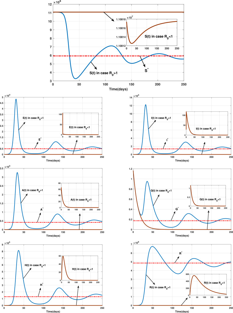
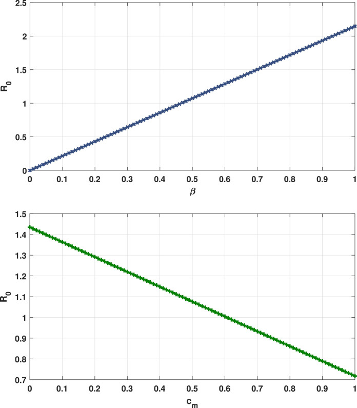
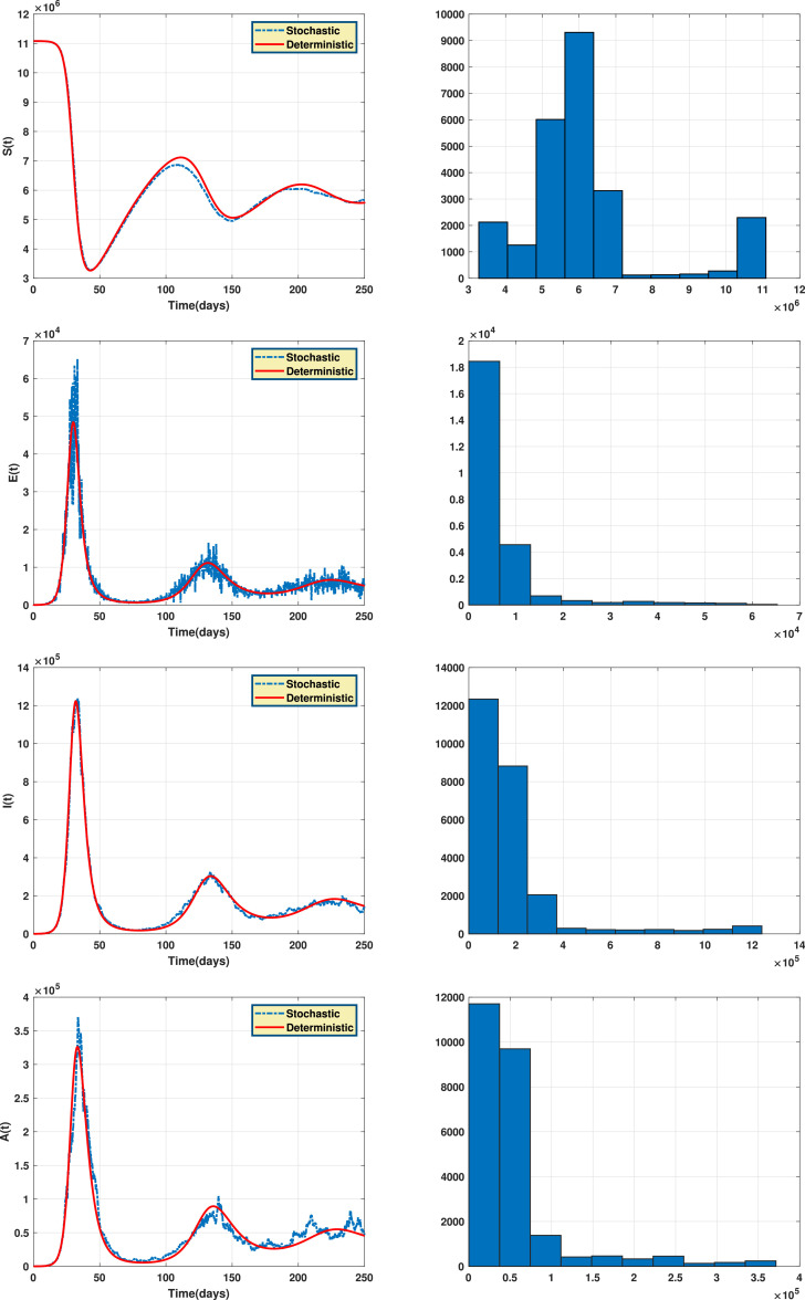
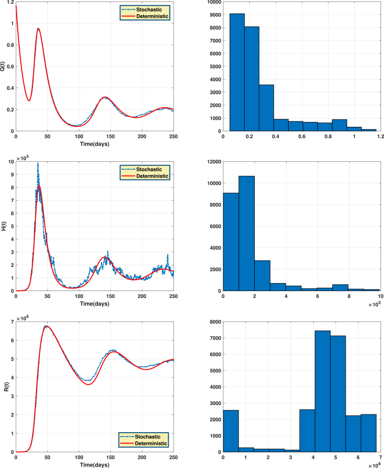
Fig. 2 shows the endemic equilibrium ${\mathcal{E}}_{*}$ and the trajectories of the solution for the case ${\mathcal{R}}_0=0.7730<1$ with $\beta =0.36$ and the case ${\mathcal{R}}_0=1.8569>1$ with $\beta =0.8648,$ when ${\sigma }_1={\sigma }_2={\sigma }_3=0$. Fig. 3 displays the reproduction number ${\mathcal{R}}_0$ for several values of $\beta \in [0,1]$ and $c_m\in [0,1],$ with ${\sigma }_1={\sigma }_2={\sigma }_3=0$. Fig. 4 and Fig. 5 display the trajectories of solution for the stochastic model (6) with ${\sigma }_1=0.15,$ ${\sigma }_2=0.32,$ ${\sigma }_3=0.26$ and the solution of the corresponding deterministic model along with the histograms of frequencies for $\mathrm{S}\left(t\right),$ $\mathrm{E}\left(t\right),$ $\mathrm{I}\left(t\right),$ $\mathrm{A}\left(t\right),$ $\mathrm{Q}\left(t\right),$ $\mathrm{H}\left(t\right)$ and $\mathrm{R}\left(t\right)$. These figures confirm that model (6) has a positive solution. Also, from the conditions

$$\frac{{\sigma }_2^2}{2}(\mathtt{p}-1)<{\alpha }_{\mathrm{I}}+{\gamma }_{\mathrm{A}}+\mu ,$$

and

$$\frac{{\sigma }_3^2}{2}(\mathtt{p}-1)<{\gamma }_{\mathrm{H}}+{\mu }_{\mathrm{I}}+\mu ,$$

for $\mathtt{p}\ge 2$ in Theorem 3, we have

$$\begin{array}{c}p=2:\frac{{\sigma }_2^2}{2}=0.0512<{\alpha }_{\mathrm{I}}+{\gamma }_{\mathrm{A}}+\mu =0.2322,\\ \frac{{\sigma }_3^2}{2}=0.0338<{\gamma }_{\mathrm{H}}+{\mu }_{\mathrm{I}}+\mu =0.1406,\end{array}$$

$$\mathrm{p}=3:{\sigma }_2^2=0.1024<0.2322,{\sigma }_3^2=0.0676<0.1406.$$

Hence, in the case $\mathtt{p}=2,$ ${\mathcal{E}}^0$ is globally asymptotically stable and in the case $\mathtt{p}=3,$ the disease-free equilibrium point ${\mathcal{E}}^0$ is exponentially 3-stable.

Fig. 2.

The trajectories of the solution for the cases ${\mathcal{R}}_0<1$ and ${\mathcal{R}}_0>1,$ when ${\sigma }_1={\sigma }_2={\sigma }_3=0$.

Fig. 3.

Reproduction number ${\mathcal{R}}_0$ for several values of $\beta$ (up) and $c_m$ (down).

Fig. 4.

The trajectories of solution for the stochastic model (6) and the solution of the corresponding deterministic model (left) along with the histograms of frequencies for the populations $\mathrm{S}\left(t\right),$$\mathrm{E}\left(t\right),$$\mathrm{I}\left(t\right)$ and $\mathrm{A}\left(t\right)$(right).

Fig. 5.

The trajectories of solution for the stochastic model (6) and the solution of the corresponding deterministic model (left) along with the histograms of frequencies for the populations $\mathrm{Q}\left(t\right),$$\mathrm{H}\left(t\right)$ and $\mathrm{R}\left(t\right)$ (right).

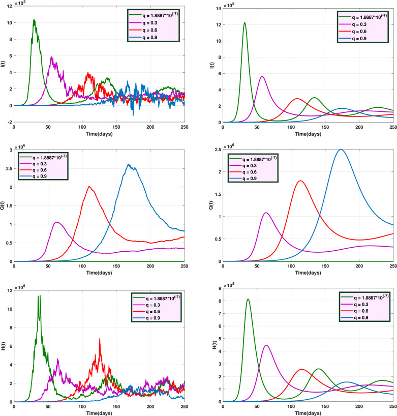
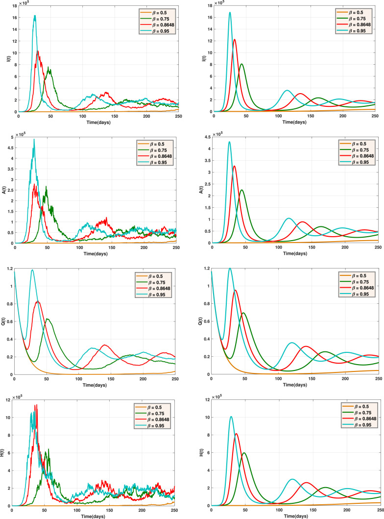
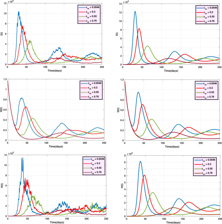
Fig. 6 shows the trajectories of $\mathrm{I}\left(t\right),$ $\mathrm{Q}\left(t\right)$ and $\mathrm{H}\left(t\right)$ for the stochastic model when ${\sigma }_1=0.2,$ ${\sigma }_2=0.15,$ ${\sigma }_3=0.22$ and the deterministic model, for several values of $q$. Fig. 7 displays the trajectories of $\mathrm{I}\left(t\right),$ $\mathrm{A}\left(t\right),$ $\mathrm{Q}\left(t\right)$ and $\mathrm{H}\left(t\right)$ for the stochastic model with ${\sigma }_1=0.3,$ ${\sigma }_2=0.2,$ ${\sigma }_3=0.15$ and the deterministic model, with different values of $\beta$. Also, Fig. 8 indicates the trajectories of $\mathrm{I}\left(t\right),$ $\mathrm{Q}\left(t\right)$ and $\mathrm{H}\left(t\right)$ for the deterministic model and the stochastic model with ${\sigma }_1=0.15,$ ${\sigma }_2=0.24,$ ${\sigma }_3=0.36$ for different values of $c_m$.

Fig. 6.

Graphs of trajectories of $\mathrm{I}\left(t\right),$$\mathrm{Q}\left(t\right)$ and $\mathrm{H}\left(t\right)$ for the stochastic model (left) and the deterministic model (right) with different values of $q$.

Fig. 7.

The trajectories of $\mathrm{I}\left(t\right),$$\mathrm{A}\left(t\right),$$\mathrm{Q}\left(t\right)$ and $\mathrm{H}\left(t\right)$ for the stochastic model (left) and the deterministic model (right) with different values of $\beta$.

Fig. 8.

The trajectories of $\mathrm{I}\left(t\right),$$\mathrm{Q}\left(t\right)$ and $\mathrm{H}\left(t\right)$ for the stochastic model (left) and the deterministic model (right) with different values of $c_m$.

6. Conclusion

A stochastic model based on some health protocols such as quarantine, social distancing and wearing masks has outlined to describe the trend of COVID-19 pandemic in a population. The existence and uniqueness of a positive global solution for the proposed model were proved. Stability analysis of the stochastic model and its special deterministic case have been discussed. In order to simulate the dynamical behaviors of the model, a step-by-step collocation method based on the Legendre polynomials was introduced. Based on the numerical result , it can be seen that considering random effects for the parameters of the model helps to depict a more realistic aspect of the disease development. Also, these results confirm that preventative actions and health strategies have a direct effect on the virus prevalence and control of the pandemic. Considering more public health strategies in the model and studying the impact of underlying diseases or other viral epidemics such as influenza, on the spread of Coronavirus, are some research directions that can be investigated for future works. Also, verifying the frequency of the disease among different age groups may be another useful subject.

CRediT authorship contribution statement

A. Babaei: Supervision, Software, Validation, Writing - review & editing. H. Jafari: Supervision, Writing - review & editing, Investigation. S. Banihashemi: Writing - review & editing, Methodology, Validation, Software. M. Ahmadi: Methodology, Validation, Software.

Declaration of Competing Interest

The authors declare no potential conflict of interests.

References

- 1.Grenfell B.T., Dobson A.P. Cambridge University Press; 1995. Ecology of infectious diseases in natural populations. [DOI] [Google Scholar]
- 2.Castillo-Chavez C., Blower S., Driessche P., van d, Kirschner D., Yakubu A.A. Springer Science and Business Media; 2002. Mathematical approaches for emerging and reemerging infectious diseases: An Introduction. [Google Scholar]
- 3.James D.M. Springer Science and Business Media; 2007. Mathematical biology: I. An introduction. [Google Scholar]
- 4.Yves E., Danhree B., Rodoumta K. Mathematical analysis of HIV/AIDS stochastic Dynamic Models. Applied Mathematical Modelling. 2016;40(21–22):9131–9151. [Google Scholar]
- 5.Babaei A., Jafari H., Ahmadi M. A fractional order HIV/AIDS model based on the effect of screening of unaware infectives. Mathematical Methods in the Applied Sciences. 2019;42(7):2334–2343. [Google Scholar]
- 6.Babaei A., Jafari H., Liya A. Mathematical models of HIV/AIDS and drug addiction in prisons. The European Physical Journal Plus. 2020:135. [Google Scholar]
- 7.Jajarmi A., Ghanbari B., Baleanu D. A new and efficient numerical method for the fractional modeling and optimal control of diabetes and tuberculosis co-existence. Chaos: An Interdisciplinary Journal of Nonlinear Science. 2019:29. doi: 10.1063/1.5112177. 093111. [DOI] [PubMed] [Google Scholar]
- 8.Khan M.A., Hammouch Z., Baleanu D. Modeling the dynamics of hepatitis E via the Caputo-Fabrizio derivative. Mathematical Modelling of Natural Phenomena. 2019;14(3):311. [Google Scholar]
- 9.Ganji R.M., Jafari H. A new approach for solving nonlinear volterra integro-differential equations with Mittag-Leffler kernel. Proceedings of the Institute of Mathematics and Mechanics. 2020;46(1):144–158. doi: 10.29228/proc.24. [DOI] [Google Scholar]
- 10.Sajjadi S.S., Baleanu D., Jajarmi A., Pirouz H.M. A new adaptive synchronization and hyperchaos control of a biological snap oscillator. Chaos, Solitons & Fractals. 2020;138:109919. [Google Scholar]
- 11.Qureshi S., Atangana A. Fractal-fractional differentiation for the modeling and mathematical analysis of nonlinear diarrhea transmission dynamics under the use of real data. Chaos, Solitons & Fractals. 2020;136:109812. [Google Scholar]
- 12.Babaei A., Jafari H., Banihashemi S., Ahmadi M. A stochastic mathematical model for COVID-19 according to different age groups. Appl Comput Math. 2021;20(1) [Google Scholar]
- 13.Babaei A., Ahmadi M., Jafari H., Liya A. A mathematical model to examine the effect of quarantine on the spread of Coronavirus. Chaos, Solitons Fractals. 2020:110418. doi: 10.1016/j.chaos.2020.110418. [DOI] [PMC free article] [PubMed] [Google Scholar]
- 14.Ali M., Shah S.T.H., Imran M., Khan A. The role of asymptomatic class, quarantine and isolation in the transmission of COVID-19. Journal of Biological Dynamics. 2020;14(1):389–408. doi: 10.1080/17513758.2020.1773000. [DOI] [PubMed] [Google Scholar]
- 15.Naik P.A., Yavuz M., Qureshi S., Zu J., Townley S. Modeling and analysis of COVID-19 epidemics with treatment in fractional derivatives using real data from Pakistan. The European Physical Journal Plus. 2020;135(10):1–42. doi: 10.1140/epjp/s13360-020-00819-5. [DOI] [PMC free article] [PubMed] [Google Scholar]
- 16.Khan M.A., Atangana A., Alzahrani A., Fatmawati The dynamics of COVID-19 with quarantined and isolation. Advances in Difference Equations. 2020:1–22. doi: 10.1186/s13662-020-02882-9. [DOI] [PMC free article] [PubMed] [Google Scholar]
- 17.Baleanu D., Mohammadi H., Rezapour S. A fractional differential equation model for the COVID-19 transmission by using the caputo-fabrizio derivative. Advances in difference equations. 2020:1–27. doi: 10.1186/s13662-020-02762-2. [DOI] [PMC free article] [PubMed] [Google Scholar]
- 18.Din A., Khan A., Baleanu D. Stationary distribution and extinction of stochastic coronavirus (COVID-19) epidemic model. Chaos, Solitons & Fractals. 2020;139:110036. doi: 10.1016/j.chaos.2020.110036. [DOI] [PMC free article] [PubMed] [Google Scholar]
- 19.Chatterjee K., Chatterjee K., Kumar A., Shankar S. Healthcare impact of COVID-19 epidemic in india: A stochastic mathematical model. Medical Journal Armed Forces India. 2020;76(2):147–155. doi: 10.1016/j.mjafi.2020.03.022. [DOI] [PMC free article] [PubMed] [Google Scholar]
- 20.Eikenberry S.E., Mancuso M., Iboi E., Phan T., Eikenberry K., Kuang Y., Kostelich E., Gumel A.B. To mask or not to mask: Modeling the potential for face mask use by the general public to curtail the COVID-19 pandemic. Infectious Disease Modelling. 2020;5:293–308. doi: 10.1016/j.idm.2020.04.001. [DOI] [PMC free article] [PubMed] [Google Scholar]
- 21.Melin P., Monica J.C., Sanchez D., Castillo O. Multiple ensemble neural network models with fuzzy response aggregation for predicting COVID-19 time series: The case of mexico. Healthcare. 2020;8(2) doi: 10.3390/healthcare8020181. [DOI] [PMC free article] [PubMed] [Google Scholar]
- 22.Ngonghala C.N., Iboi E., Eikenberry S., Scotch M., MacIntyre C.R., Bonds M.H., Abba B.G. Mathematical assessment of the impact of non-pharmaceutical interventions on curtailing the 2019 novel coronavirus. Mathematical Biosciences. 2020;325:108364. doi: 10.1016/j.mbs.2020.108364. [DOI] [PMC free article] [PubMed] [Google Scholar]
- 23.Wu J., Tang B., Bragazzi N.L., Nah K., McCarthy Z. Quantifying the role of social distancing personal protection and case detection in mitigating COVID-19 outbreak in ontario, canada. Journal of Mathematics in Industry. 2020;10(1):1–12. doi: 10.1186/s13362-020-00083-3. [DOI] [PMC free article] [PubMed] [Google Scholar]
- 24.Driessche P.D.V., Watmough J. Reproduction numbers and sub-threshold endemic equilibria for compartmental models of disease transmission. Math Biosci. 2002;180:29—48. doi: 10.1016/s0025-5564(02)00108-6. [DOI] [PubMed] [Google Scholar]
- 25.Mao X. Horwood; Chichester: 1997. Stochastic Differential Equations and Applications. [Google Scholar]
- 26.Babaei A., Jafari H., Banihashemi S. A collocation approach for solving time-fractional stochastic heat equation driven by an additive noise. Symmetry. 2020:12. doi: 10.3390/sym12060904. [DOI] [Google Scholar]
- 27.Afanasiev V.N., Kolmanowskii V.B., Nosov V.R. Kluwer Academic; Dordrecht: 1996. Mathematical Theory of Control Systems Design. [Google Scholar]
- 28.Canuto C., Hussaini M.Y., Quarteroni A., Zang T.A. Spectral methods: Fundamentals in single domains. Springer-Verlag. 2006 [Google Scholar]
- 29.Resmawan R., Yahya L. Sensitivity analysis of mathematical model of coronavirus disease (COVID-19) transmission. CAUCHY-Jurnal Matematika Murni dan Aplikasi. 2020;6:91–99. [Google Scholar]
- 30.Shaikh A., Shaikh I.N., Sooppy Nisar K. A mathematical model of COVID-19 using fractional derivative: Outbreak in india with dynamics of transmission and control. Advances in Difference Equations. 2020 doi: 10.1186/s13662-020-02834-3. [DOI] [PMC free article] [PubMed] [Google Scholar]
- 31.Tang B., Wang X., Li Q., Bragazzi N.L., Tang S., Xiao Y., et al. Estimation of the transmission risk of the 2019-ncov and its implication for public health interventions. Journal of Clinical Medicine. 2020;9(2) doi: 10.3390/jcm9020462. [DOI] [PMC free article] [PubMed] [Google Scholar]