Modeling regional changes in dynamic stability during sleep and wakefulness

Abstract

Global brain states are frequently placed within a unidimensional continuum by correlational studies, ranging from states of deep unconsciousness to ordinary wakefulness. An alternative is their multidimensional and mechanistic characterization in terms of different cognitive capacities, using computational models to reproduce the underlying neural dynamics. We explore this alternative by introducing a semi-empirical model linking regional activation and long-range functional connectivity in the different brain states visited during the natural wake-sleep cycle. Our model combines functional magnetic resonance imaging (fMRI) data, in vivo estimates of structural connectivity, and anatomically-informed priors to constrain the independent variation of regional activation. The best fit to empirical data was achieved using priors based on functionally coherent networks, with the resulting model parameters dividing the cortex into regions presenting opposite dynamical behavior. Frontoparietal regions approached a bifurcation from dynamics at a fixed point governed by noise, while sensorimotor regions approached a bifurcation from oscillatory dynamics. In agreement with human electrophysiological experiments, sleep onset induced subcortical deactivation with low correlation, which was subsequently reversed for deeper stages. Finally, we introduced periodic forcing of variable intensity to simulate external perturbations, and identified the key regions relevant for the recovery of wakefulness from deep sleep. Our model represents sleep as a state with diminished perceptual gating and the latent capacity for global accessibility that is required for rapid arousals. To the extent that the qualitative characterization of local dynamics is exhausted by the dichotomy between unstable and stable behavior, our work highlights how expanding the model parameter space can describe states of consciousness in terms of multiple dimensions with interpretations given by the choice of anatomically-informed priors.

1. Introduction

The human brain is a complex system comprised by 10¹⁰ nonlinear units (neurons) interacting in 10¹⁵ sites (synapses) (Sporns et al., 2005). Considering such an astonishing level of complexity and heterogeneity, it is surprising that the global dynamics of the brain self-organize into a discrete set of well-defined states (Tart, 1971; Tassi and Muzet, 2001), and that these states are frequently placed along a unidimensional continuum (Bayne et al., 2016).¹ This continuum corresponds to the level of consciousness, which is reduced in states such as sleep, general anesthesia or post-comatose disorders. The intuition behind the concept of “level of consciousness” is that consciousness is graded and uniform, and that one can be more or less conscious relative to the baseline given by conscious wakefulness. Behavioral and neurobiological characterizations of global states are aligned with this intuition; for instance, clinicians use unidimensional scales to assess the level of consciousness in brain injured patients (Sternbach, 2000), and apply algorithms to electroencephalography (EEG) data to monitor the depth of anesthesia (Rosow and Manberg, 2001).

This view has been recently challenged by the proposal that multiple independent levels of analysis are required to describe states of consciousness (Bayne et al., 2016, 2017), with similar proposals put forward for the specific case of human sleep (Hobson and Pace-Schott, 2002; Windt et al., 2016; Song and Tagliazucchi, 2019). The levels proposed by Bayne and colleagues distinguish between functional and sensory dimensions. The first include the availability of information for modules associated with specific cognitive functions, which is generally widespread during conscious wakefulness (Dehaene and Naccache, 2001), but can be compromised during other states of consciousness (Bartolomei and Naccache, 2001; Berkovitch et al., 2017). Examples of the second include the gating of sensory content and the binding of low-level features into objects belonging to well-defined categories (Treisman, 1998). It is expected that deficits in different dimensions relate to specific regions or networks of regions, for instance, global information availability is linked to the activation of fronto-parietal regions (Sergent and Dehaene, 2004), while perceptual deficits could implicate multiple regions along the hierarchy of sensory processing. Even in the absence of sensory stimulation and overt behavior, functional magnetic resonance imaging (fMRI) reveals that the brain is organized into independent functional patterns, known as resting state networks (RSNs) (Damoiseaux et al., 2006). RSNs approximately match different task-elicited activity patterns, including patterns associated with the independent levels of analysis proposed by Bayne and colleagues. Thus, states of consciousness could be characterized by their profile of RSN-specific changes, as opposed to single metrics related to functional integration and complexity (Tononi and Edelman, 1998). In particular, changes in the gating of sensory content and in global information availability can be interpreted in terms of parameters associated with sensory (e.g. visual) and fronto-parietal RSN, respectively.

Functional connectivity (FC) within RSNs is constrained by the structural connectivity (SC) of the brain (Greicius et al., 2009; Van Den Heuvel et al., 2009; Haimovici et al., 2013), which is preserved in reversible states such as sleep and anesthesia. The interplay between local dynamics and long-range SC must be disentangled to describe states of consciousness in terms of the functional and sensory domains associated with different RSNs. Network models of whole-brain activity can be implemented to disentangle these contributions and investigate the effect of external perturbations (Honey et al., 2007, 2009; Ghosh et al., 2008; Haimovici et al., 2013; Taylor et al., 2014; Sanz-Leon et al., 2015; Spiegler et al., 2016; Breakspear, 2017; Fukushima and Sporns, 2018). These models can be used to compute simulated FC patterns from brain activity time series generated by the differential equations governing local dynamics, coupled by in vivo diffusion tensor imaging (DTI) estimates of SC. A set of interpretable parameters can then be adjusted to optimize the similarity between the simulated and empirical FC patterns obtained during different states of consciousness. For instance, when applied to the stages of human sleep, these models show promise to contrast hypotheses concerning the origin of spontaneous brain activity across the wake-sleep cycle (Jobst et al., 2017), as well as to predict the behavior of brain activity in response to external and internal driving events (Deco et al., 2017, 2018a).

The use of homogeneous parameters helps to reduce model complexity, allowing the fast and straightforward optimization of simulated FC. While low complexity models are useful to provide conceptual insights, they are limited to investigate regional dynamics that can be traced back to known neurophysiological systems embedded within different RSNs, and their associated cognitive functions. In particular, their usefulness is limited to provide a multidimensional characterization of states of consciousness, understood as a description capable of taking multiple and seemingly independent factors into account, such as the representation of sensory content from different modalities, or alterations in the different functions comprised by human cognition. Homogeneous model parameters are also limiting for the purpose of rehearsing anatomically localized in silico stimulation protocols to restore the dynamics seen during conscious wakefulness (Deco et al., 2019), since expecting an uniform interaction between baseline activity and external stimulation is likely an oversimplification (Opitz et al., 2018). To overcome these limitations, we developed whole-brain models of fMRI activity recorded during the human wake-sleep cycle incorporating regional parameters constrained by anatomical priors, i.e. priors constraining the spatial heterogeneity of the parameters. These parameters govern supercritical Hopf bifurcations between activated synchronous states and quiescent stable states with noisy fluctuations.

This paper is structured as follows. First, we introduce the computational model and the sources of empirical data, including SC, FC and the anatomical priors to constrain regional parameter variation. Next, we apply genetic algorithms for the optimization of simulated FC in terms of its similarity to the empirical FC obtained during wakefulness, and determine the anatomical prior giving the maximal similarity. We estimate the optimal regional parameters for wakefulness and the different stages of human sleep. Finally, we investigate the capacity of local periodic forcing to transition the model dynamics towards conscious wakefulness, with the purpose of determining whether heterogeneous local bifurcation parameters result in qualitatively different responses upon stimulation delivered at multiple brain regions.

2. Materials and methods

2.1. Participants and experimental protocol

A cohort of 63 healthy subjects participated in the original experiments (36 females, mean ± SD age of 23.4 ± 3.3 years). Written informed consent was obtained from all subjects. The experimental protocol was approved by the local ethics committee (Goethe-Universität Frankfurt, Germany, protocol number: 305/07). The subjects were reimbursed for their participation. All experiments were conducted in accordance with the relevant guidelines and regulations, and the Declaration of Helsinki.

The participants entered the scanner in the evening (within half an hour of 7 p.m.) and underwent a resting state fMRI session with simultaneous EEG acquisition lasting for 52 min. Participants were not instructed to fall asleep, but were asked to relax, close their eyes and not actively fight the onset of sleep. Lights were dimmed in the scanner room and subjects were shielded from scanner noise using earplugs. The day of the study all participants reported a wake-up time between 5:00 a.m. and 11:00 a.m., and a sleep onset time between 10:00 p.m. and 2:00 a.m. for the night prior to the experiment. Sleep diaries confirmed that these values were representative of the 6 days prior to the experiment.

Sleep staging was based on simultaneously acquired polysomnography data and performed according to the standard rules of the American Academy of Sleep Medicine (Berry et al., 2012). For the included participants the mean (±SD) durations of contiguous sleep epochs were 12.37 ± 6.61 min for wakefulness, 8.52 ± 2.83 min for N1, 14.69 ± 5.72 min for N2 and 16.56 ± 8.39 min for N3.

2.2. Simultaneous fMRI and EEG data collection

EEG via a cap (modified BrainCapMR, Easycap, Herrsching, Germany) was recorded continuously during fMRI acquisition (1505 vol of T2*-weighted echo planar images, TR/TE = 2080 ms/30 ms, matrix 64 × 64, voxel size 3 × 3 × 2 mm³, distance factor 50%; FOV 192 mm²) with a 3 T S Trio (Erlangen, Germany). An optimized polysomnographic setting was employed (chin and tibial EMG, ECG, EOG recorded bipolarly [sampling rate 5 kHz, low pass filter 1 kHz] with 30 EEG channels recorded with FCz as the reference [sampling rate 5 kHz, low pass filter 250 Hz]. Pulse oxymetry and respiration were recorded via sensors from the Trio [sampling rate 50 Hz]) and MR scanner compatible devices (BrainAmp MR+, BrainAmpExG; Brain Products, Gilching, Germany), facilitating sleep scoring during fMRI acquisition.

MRI and pulse artifact correction were performed based on the average artifact subtraction (AAS) method (Allen et al., 1998) as implemented in Vision Analyzer 2 (Brain Products, Germany) followed by objective (CBC parameters, Vision Analyzer) ICA-based rejection of residual artifact-laden components after AAS resulting in EEG with a sampling rate of 250 Hz. EEG artifacts due to motion were detected and eliminated using an ICA procedure implemented in Vision Analyzer 2. Previous publications based on this dataset can be consulted for further details (e.g. Tagliazucchi et al., 2012).

2.3. fMRI data preprocessing

Using Statistical Parametric Mapping (SPM8, www.fil.ion.ucl.ac.uk/spm), Echo Planar Imaging (EPI) data were realigned, normalized (MNI space) and spatially smoothed (Gaussian kernel, 8 mm³ full width at half maximum). Data was then re-sampled to 4 × 4 × 4 mm resolution. Note that re-sampling introduces local averaging of Blood Oxygen Level Dependent (BOLD) signals, which were eventually averaged over larger cortical and sub-cortical regions of interest, determined by the automatic anatomic labeling (AAL) atlas (Tzourio-Mazoyer et al., 2002). Cardiac, respiratory (both estimated using the RETROICOR method [Glover et al., 2000]) and motion-induced noise (three rigid body rotations and translations, as well as their first 3 temporal derivatives, resulting in 24 motion regressors) (Friston et al., 1996) were regressed out by retaining the residuals of the best linear least square fit. Data was band-pass filtered in the range 0.01–0.1 Hz (Cordes et al., 2001) using a sixth order Butter-worth filter.

2.4. DWI data collection and processing

The structural connectome was obtained applying diffusion tensor imaging (DTI) to diffusion weighted imaging (DWI) recordings from 16 healthy right-handed participants (11 men and 5 women, mean age: 24.75 ± 2.54 years) recruited online at Aarhus University, Denmark. Subjects with psychiatric or neurological disorders (or a history thereof) were excluded from participation. The MRI data (structural MRI, DTI) were recorded in a single session on a 3 T S Skyra scanner. The following parameters were used for the structural MRI T1 scan: voxel size of 1mm³; reconstructed matrix size 256 × 256; echo time (TE) of 3.8 ms and repetition time (TR) of 2300 ms. DWI data were collected using the following parameters: TR = 9000 ms, TE = 84 ms, flip angle = 90°, reconstructed matrix size of 106 × 106, voxel size of 1.98 × 1.98 mm with slice thickness of 2 mm and a bandwidth of 1745 Hz/Px.

Furthermore, the data were recorded with 62 optimal nonlinear diffusion gradient directions at b = 1500 s/mm². Approximately one non-diffusion weighted image (b = 0) per 10 diffusion-weighted images was acquired. Additionally, the DTI images were recorded with different phase encoding directions. One set was collected applying anterior to posterior phase encoding direction and the second one was acquired in the opposite direction. The AAL template was used to parcellate the entire brain into 90 regions (76 cortical regions and 14 subcortical regions). The parcellation contained 45 regions in each hemisphere. To co-register the EPI image to the T1-weighted structural image, the linear registration tool from the FSL toolbox (www.fmrib.ox.ac.uk/fsl, FMRIB, Oxford) (Jenkinson et al., 2002) was employed. The T1-weighted images were co-registered to the T1 template of ICBM152 in MNI space. The resulting transformations were concatenated, inverted and further applied to warp the AAL template from MNI space to the EPI native space, where the discrete labeling values were preserved by applying nearest-neighbor interpolation. SC networks were constructed following a three-step process. First, the regions of the whole-brain network were defined using the AAL template. Second, the connections between nodes in the whole-brain network (i.e., edges) were estimated using probabilistic tractography for each participant. Third, results were averaged across participants.

Data preprocessing was performed using FSL diffusion toolbox (Fdt) with default parameters. Following this preprocessing, the local probability distributions of fiber directions were estimated at each voxel (Behrens et al., 2003). The probtrackx tool in Fdt was used to provide automatic estimation of crossing fibers within each voxel, which has been shown to significantly improve the tracking sensitivity of non-dominant fiber populations in the human brain (Behrens et al., 2007). The connectivity probability from a seed voxel i to another voxel j was defined by the proportion of fibers passing through voxel i that reached voxel j (sampling of 5000 streamlines per voxel [Behrens et al., 2007]). All the voxels in each AAL parcel were seeded (i.e. gray and white matter voxels were considered). This was extended from the voxel level to the region level, i.e. in a parcel consisting of n voxels, 5000 × n fibers were sampled. The connectivity probability P_ij from region i to region j was calculated as the number of sampled fibers in region i that connected the two regions, divided by 5000 × n, where n represents the number of voxels in region i. The resulting SC matrices were thresholded at 0.1% (i.e. a minimum of five streamlines).

Due to the dependence of tractography on the seeding location, the probability from i to j was not necessarily equivalent to that from j to i. However, these two probabilities were highly correlated across the brain for all participants (r > 0.70, p < 10⁻⁵⁰). As the directionality of connections cannot be determined using diffusion MRI, the unidirectional connectivity probability P_ij between regions i and j was defined by averaging these two connectivity probabilities. This unidirectional connectivity was considered a measure of SC between the two areas, with C_ij = C_ji. The regional connectivity probability was calculated using inhouse Perl scripts. For both phase encoding directions, 90 × 90 symmetric weighted networks were constructed based on the AAL parcellation, and normalized by the number of voxels in each AAL region, thus representing the SC network organization of the brain of each participant. Finally, the data was averaged across participants.

2.5. Group averaged FC matrices

fMRI signals were detrended and demeaned before band-pass filtering in the 0.04–0.07 Hz range (Glerean et al., 2012). The frequency range of 0.04–0.07 Hz was chosen because when mapped to the gray matter this frequency band was shown to contain more reliable and functionally relevant information compared to other frequency bands, and to be less affected by noise (Biswal et al., 1995; Glerean et al., 2012; Achard et al., 2006; Buckner et al., 2009). Subsequently, the filtered time series were transformed to z-scores. For each sleep stage, 15 participants were selected based on the presence of uninterrupted epochs of that sleep stage lasting more than 200 samples. Afterwards, the FC matrix was defined as the matrix of Pearson correlations between the fMRI signals of all pairs of regions of interest (ROIs) in the AAL template. To avoid confounds related to the length of the time series, the correlations were computed using only the first 200 vol of each sleep stage. Fixed-effect analysis was used to obtain group-level FC matrices, meaning that the Fisher’s R-to-z transform (z = atanh(R)) was applied to the correlation values before averaging over participants within each sleep stage.

2.6. Computational whole-brain model

The general approach followed to construct the semi-empirical model is presented in the left panel of Fig. 1. Two different sources of empirical data were combined in a model where local dynamics are given by weakly interacting nonlinear oscillators. DTI data provided an estimate of SC between the oscillators, fMRI was used to estimate the intrinsic oscillation frequency of the local dynamics, and also provided empirical FC matrices that were used to fit the simulations, and RNSs determined a natural prior to group the nodes that contributed independently to the final local bifurcation parameters.

Fig. 1.

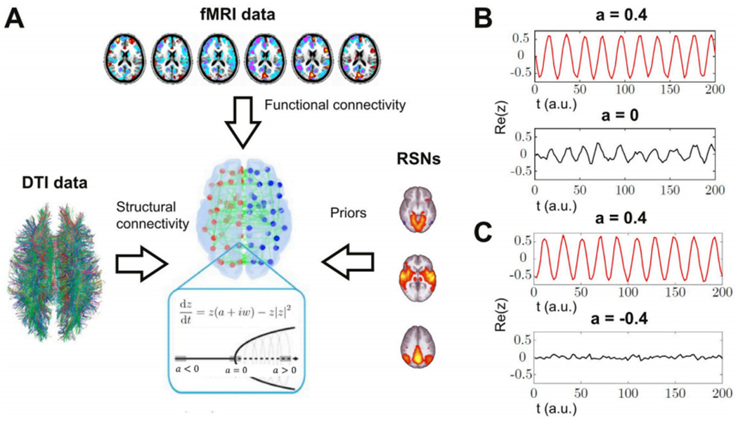
Procedure followed to construct the whole-brain model and a simplified example of the dynamics of two coupled oscillators. A) The model incorporates DTI data to define the SC between the non-linear oscillators, fMRI data to determine the intrinsic oscillation frequency of each node and the empirical FC that is fitted in the simulations, and RSNs as an anatomical prior to define the groups of nodes that contribute independently to the local bifurcation parameters. Dynamics are given by the normal form of a supercritical Hopf bifurcation (the equations and bifurcation diagram are provided in the inset). B-C) Example of two coupled oscillators with different bifurcation parameters. Panel B shows how oscillatory dynamics (a > 0) can induce oscillations in a critical node (a = 0) due to their coupling, while panel C shows that noisy dynamics at the fixed point (a < 0) prevents the synchronization with the oscillating node (a > 0). Re(z) stands for the real part of the simulated time series, which corresponds to the modeled fMRI signal.

The implemented whole-brain model consisted of a network of nonlinear oscillators coupled by SC. Each oscillator represents the dynamics at one of the 90 brain regions in the AAL template. The key neurobiological assumption is that dynamics of macroscopic neural masses can range from fully synchronous (i.e. activated state) to a stable asynchronous state governed by random fluctuations. A secondary assumption is that fMRI can capture the dynamics from both regimes (mediated by hemodynamic changes at a slower temporal scale, allowing to neglect the effect of signal transmission delays) with sufficient fidelity to be modeled by the equations.

Based on previous work (Jobst et al., 2017; Deco et al., 2017, 2018), the nonlinear oscillators were modeled by the normal form of a super-critical Hopf bifurcation. This type of bifurcation can change the qualitative nature of the solutions from a stable fixed point in phase space towards a limit cycle allowing the model to present self-sustained oscillations. While models of higher complexity could display analogous behavior, the normal form of a Hopf bifurcation was chosen for reasons of simplicity and generality, since it includes the minimal number of non-linearities representing this range of dynamics.

Without coupling, the local dynamics of brain region j was modeled by the complex equation:

$$\frac{{\text{dz}}_{\text{j}}}{\text{dt}}=\left[\text{a+i}{\omega }_{\text{j}}\right]{\text{z}}_{\text{j}}-{\text{z}}_{\text{j}}{|{\text{z}}_{\text{j}}|}^2$$ (1)

In this equation z is a complex-valued variable (z_j = x_j + iy_j), and ω_j is the intrinsic oscillation frequency of node j. The intrinsic frequencies ranged from 0.04 to 0.07 Hz and were determined by the averaged peak frequency of the bandpass-filtered fMRI signals of each individual brain region.

The parameter a is known as the bifurcation parameter and controls the dynamical behavior of the system. Fora < 0 the phase space presents a unique stable fixed point at z_j = 0, thus the system asymptotically decays towards this point. For a > 0 the stable fixed point changes its stability, giving rise to a limit cycle and to self-sustained oscillations with frequency f_j = ω_j/2π and amplitude proportional to the square root of a. (Deco et al., 2017).

The coordinated dynamics of the resting state activity are modeled by introducing coupling determined by the SC. Nodes i and j are coupled by C_ij (the i,j entry of the SC matrix). To ensure oscillatory dynamics for a > 0, the SC matrix was scaled to a maximum of 0.2 (weak coupling condition) (Deco et al., 2017). In full form, the coupled differential equations of the model are the following:

$$\begin{gathered} \frac{{\text{dx}}_{\text{j}}}{\text{dt}}=\frac{\text{dRe}\left({\text{z}}_{\text{j}}\right)}{\text{dt}}=\left[{\text{a}-\text{x}}_{\text{j}}^2-{\text{y}}_j^2\right]{\text{x}}_{\text{j}}-{\omega }_{\text{j}}{\text{y}}_{\text{j}}+\text{G}\underset{\text{i}}{\Sigma }{\text{C}}_{\text{ij}}\left({\text{x}}_{\text{i}}{-\text{x}}_{\text{j}}\right)+\beta {\eta }_{\text{j}}\left(\text{t}\right) \\ \frac{{\text{dy}}_{\text{j}}}{\text{dt}}=\frac{\text{dIm}\left({\text{z}}_{\text{j}}\right)}{\text{dt}}=\left[{\text{a}-\text{x}}_{\text{j}}^2-{\text{y}}_j^2\right]{\text{y}}_{\text{j}}+{\omega }_{\text{j}}{\text{x}}_{\text{j}}+\text{G}\underset{\text{i}}{\Sigma }{\text{C}}_{\text{ij}}\left({\text{y}}_{\text{i}}{-\text{y}}_{\text{j}}\right)+\beta {\eta }_{\text{j}}\left(\text{t}\right) \end{gathered}$$ (2)

The parameter G represents a global coupling factor that scales SC equally for all the nodes. These equations were integrated to simulate empirical fMRI signals using the Euler-Maruyama algorithm with a time step of 0.1 s η_j(t) represents additive Gaussian noise. When a is close to the bifurcation (a^~0) the additive gaussian noise gives rise to complex dynamics as the system continuously switches between both sides of the bifurcation.

To illustrate the dynamical behavior of coupled nonlinear oscillators, we show the results obtained from two nodes in Fig. 1B and C. We present two representative cases: 1) one node (node 1) is in the dynamical regime of self-sustained oscillations (a = 0.4), and the other node (node 2) is close to the bifurcation (a^~0); and 2) node 1 as before (a > 0) while node 2 is at the stable fixed point regime (a = −0.4). For both examples, the value of the coupling coefficient C₁₂ was set to 0.01. In the first case it is apparent that the coupling with synchronous dynamics at node 1 induces oscillations in node 2, while this does not happen when node 2 is at the fixed-point regime. This example illustrates how the bifurcation parameter, which is interpreted as determining the level of regional activation, relates to the FC between the nodes, i.e. FC increases for coupled nodes when at least one of them is in the oscillatory regime and the other close to the bifurcation.

Priors for regional variations in the bifurcation parameters.

We extended previous modeling efforts by introducing additional parameters accounting for regional variations in the dynamical regime of the nodes. Introducing an independent bifurcation parameter for each individual node could result in a costly optimization procedure prone to overfitting. Thus, we considered priors to reduce the dimensionality by grouping the AAL nodes into possibly overlapping sets. We consider n of such groups, g₁, ……, g_n, each contributing an independent coefficient Δa₁, ……, Δa_n to the final bifurcation parameter of the node, which is computed as the linear combination:

$${\text{a}}_{\text{i}}=\underset{j=1}{\overset{\text{n}}{\Sigma }}\Delta {\text{a}}_{\text{j}}{\text{l}}_{{\text{g}}_{\text{j}}}\left(\text{i}\right)$$ (3)

where 1_gj is the indicator function of set g_j (i.e. 1 if the node belongs to g_j and 0 otherwise).

By introducing priors, we constrain how different groups of nodes can contribute independently to the final bifurcation parameters, while allowing for regional variation depending on the precise definition of the sets g_j. We explored five different priors: the heuristic prior, based on identifying the blocks of regions with high correlation in the empirical FC matrix (determined from the crossings of a threshold given by the mean correlation, see Fig. S1 in the supplementary information), the ad-hoc equipartition prior (grouping the nodes in six regular partitions), the RSN prior (grouping the nodes by RSN membership), the random prior (randomly assigning the nodes to the groups) and the homogeneous prior (only one group containing all the nodes). The different priors are compared in the supplementary information (Figs. S2 and S3). All codes for the computational model and parameter optimisation are available at https://github.com/iperezipina/Opt_HopfGenetic

2.7. Group simulated FC matrices

Once the coupling scaling factor G and the coefficientsΔa_i of the n groups of nodes are determined, our model simulates 10 Hz sampled time series that can be used to compute FC matrices of each state. To be compared with the empirical group averaged FC matrices described above, we processed the simulated signals as the empirical data to obtain the group simulated FC. First, we subsampled simulated time series to 0.5 Hz (2 samples per second, as in the empirical data), keeping the final time series 3000 samples long, since the empirical data was obtained from 15 subjects with 200 samples each and then bandpass filtered in the 0.04–0.07 Hz range. Finally, we computed the simulated FC as the Pearson’s correlation coefficient between the time series of each node.

2.8. Goodness of fit: structure similarity index (SSIM)

Our goal was to fit the model to the data recorded during different sleep stages by inferring the optimal coefficients Δa_j. Different metrics can be used to determine the goodness of fit (GoF), such as the euclidean or correlation distance between the FC matrices, or the mean and standard deviation of the Kuramoto order parameter computed from the Hilbert transform of the time series (Jobst et al., 2017). We opted to use a metric that balances sensitivity to absolute (e.g. euclidean distance) and relative (e.g. correlation distance) differences between the FC matrices, termed the structure similarity index (SSIM) (Zhou et al., 2004). This metric is based on three observables computed from a 2D array of values: the luminance, the contrast and the structure. The final distance between two arrays x and y is obtained from the product of the three terms l(x,y), c(x, y) and s(x, y) related to each of the observables:

$$\begin{gathered} \text{SSIM}\left(\text{x},\text{y}\right)=\text{l}{\left(\text{x},\text{y}\right)}^{\alpha }.\text{c}{\left(\text{x},\text{y}\right)}^{\beta }.\text{s}{\left(\text{x},\text{y}\right)}^{\gamma } \\ \text{l}\left(\text{x,y}\right)=\frac{2{\mu }_{\text{x}}{\mu }_{\text{y}}+{\text{C}}_1}{{\mu }_{\text{x}}^2+{\mu }_{\text{y}}^2+{\text{C}}_1} \\ \text{c}\left(\text{x},\text{y}\right)=\frac{{\sigma }_{\text{x}}{\sigma }_{\text{y}}+{\text{C}}_2}{{\sigma }_{\text{x}}^2+{\sigma }_{\text{y}}^2+{\text{C}}_2} \\ \text{s}\left(\text{x},\text{y}\right)=\frac{{\sigma }_{\text{xy}}+{\text{C}}_3}{{\sigma }_{\text{x}}{\sigma }_{\text{y}}+{\text{C}}_3} \end{gathered}$$ (4)

The exponents of each term are commonly set to α = β = γ = 1 , C₁ = (0.01 L)², C₂ = (0.03 L)² and C₃ = C₂/2, with L depending on the dynamic range of the matrix. For correlation matrices between −1 and 1, L is set to 1 (Wang et al., 2004). The SSIM ranges between 0 (lowest similarity) and 1 (highest similarity). The variables μ_x,μ_y, σ_x,σ_y and σ_xy are the local means, standard deviations, and cross-covariances of images x, y, respectively. We define goodness of fit between two FC matrices as GoF = SSIM.

2.9. Scaling of the structural coupling

The parameter G was selected by exhaustively exploring the model using a homogeneous bifurcation parameter (i.e. the same bifurcation parameter for all nodes). The GoF between empirical and simulated FC for wakefulness was computed over a 100 × 100 grid in parameter space, with the bifurcation parameter a in the [−0.2, 0.2] interval and G in the [0, 3] interval. Before computing the simulated FC, the time series from the model were resampled to one sample per 2 s (final simulated time series are 3000 samples long, since empirical data was obtained from 15 subjects with 200 samples each) and bandpass filtered in the 0.04–0.07 Hz range. After averaging 50 independent repetitions we found the absolute maximum of GoF in a = 0 and G = 0.5, with a mean GoF of 0.3 (i.e. 30% similarity according to the SSIM). These results were used as initial conditions in the following model that incorporated regional variation in the bifurcation parameters, fixing G = 0.5 in further analyses.

2.10. Genetic algorithm for parameter optimization

After determining G, the n coefficients Δa₁ ……, Δa_n remain to be optimized. The exhaustive exploration of the parameter space is computationally prohibitive, thus we resorted to the application of a genetic algorithm from Matlab Global Optimization Toolbox (https://www.mathworks.com/help/gads/ga.html) to optimize the co-efficients. This stochastic optimization procedure is inspired in biological evolution, and is based on an algorithmic representation of natural selection consisting of letting the most adapted individuals prevail in the next generation, spreading the genes responsible for their better adaptation. In terms of this algorithmic representation, the most adapted individuals are those that minimize a target fitness function (TFF) that in our work is defined as TFF = 1-GoF. The algorithm starts with a generation of 10 sets of parameters (“individuals”) chosen randomly close to zero, and generates a population of outputs with their corresponding TFF. A score proportional to the TFF is assigned to each individual. Afterwards, a group of individuals is chosen based on their score (“parents”), and the operations of crossover, mutation and elite selection are applied to them to create the next generation. These three mechanisms can be briefly described as follows: 1) elite selection occurs when an individual of a generation shows an extraordinarily low TFF in comparison with the other individuals, thus this solution is replicated without changes in the next generation; 2) the crossover operator consists of combining two selected parents to obtain a new individual that carries information from each parent to the next generation; 3) the mutation operator changes one selected parent to induce a random alteration in an individual of the next generation. In our implementation, 20% of the new generation was created by elite selection, 60% by crossover of the parents and 20% by mutation. A new population is thus generated (“offspring”) that is used iteratively as the next generation until at least one of the following halting criteria is met: 1) 200 generations are reached (i.e. limit of iterations), 2) the best solution of the population remains constant for 50 generations, 3) the average TFF across the last 50 generation is less than 1e⁻⁶. We restricted the size of the population to N = 10 in order to obtain 100 runs of the optimization procedure for each case, resulting in affordable simulation time. In Fig.S7 the relationship between N and the mean/distribution of solutions generated with the genetic algorithm are displayed.

The output of the genetic algorithm contains the simulated FC with the highest FC, and the n optimal coefficients Δa₁ ……, Δa_n, representing the independent contributions of the groups of nodes to the local bifurcation parameters. A schematic representation of the implemented genetic algorithm is shown in Fig. 2.

Fig. 2.

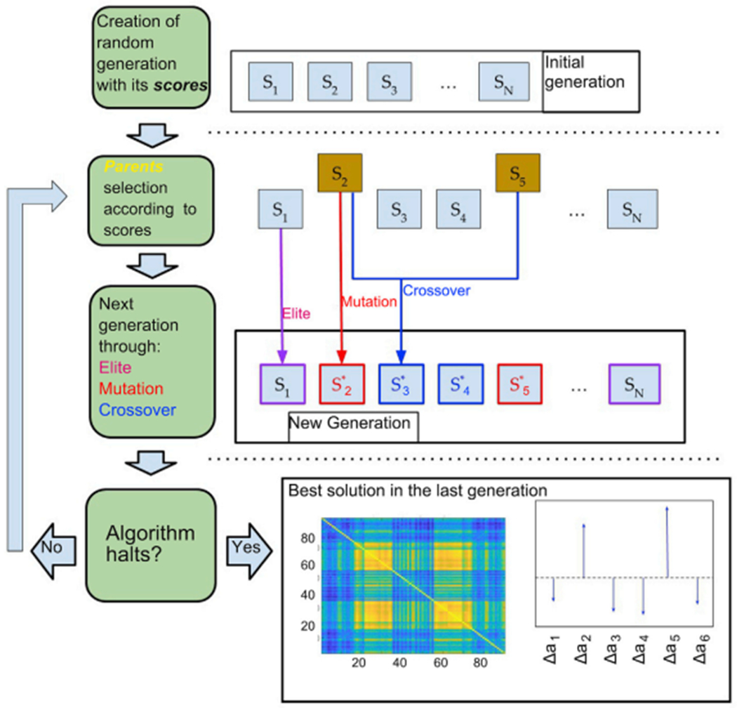
Schematic of the genetic algorithm implemented to optimize the group coefficients. A population of 10 individuals (i.e. sets of parameters) with their corresponding scores (TFF of the empirical vs. simulated FC) is first generated, followed by a selection of parents based on their scores. A new generation of individuals is then generated by elite selection, crossover from the parents and mutation. This step is iteratively applied until at least one of the halting criteria is met. When finished, the algorithm outputs the optimal coefficients together with the TFF and the simulated FC.

2.11. Modeling transitions between brain states

The optimization procedure was performed for the four brain states, ranging from wakefulness to deep sleep. In each case six parameters were obtained, corresponding to the coefficients in Eq. (3). After obtaining the optimal parameters, we modeled an external oscillatory perturbation and investigated whether it could induce a transition between deep sleep (N3) and wakefulness. The stimulus was represented as an external additive periodic forcing term incorporated to the equation of the j node, given by ${\text{F}}_{\text{j}}={\text{F}}_{0_{\text{j}}}\text{cos}\left({\omega }_{\text{j}}\text{t}\right)$, where F_0j is the coefficient of the forcing and ω_j is the natural frequency of the node j. The effects of the forcing were investigated systematically for all 45 pairs of homotopic regions in the AAL atlas. The purpose of this perturbation was to model the effects of transcranial alternating current stimulation (tACS).

This forcing was initially applied for the parameters chosen to reproduce deep sleep FC, with the forcing amplitude (F_0j ) of node j and its homotopic pair being parametrically increased from 0 to 2 in steps of 0.05 (averaging 100 independent simulations for each node pair and F_0j value). For each value of F_0j the FC matrix was computed and its similarity to the wakefulness FC was determined as follows,

$$\Delta {\text{GoF}}_{\text{norm}}=\frac{\text{GoF}\left({\text{FC}}_{{\text{sim}}_{\text{W}}},{\text{FC}}_{{\text{emp}}_{\text{W}}}\right)-\text{GoF}\left({\text{FC}}_{{\text{sim}}_{\text{f}}},{\text{FC}}_{{\text{emp}}_{\text{W}}}\right)}{\text{GoF}\left({\text{FC}}_{{\text{sim}}_{\text{W}}},{\text{FC}}_{{\text{emp}}_{\text{W}}}\right)-\text{GoF}\left({\text{FC}}_{{\text{sim}}_{\text{N3}}},{\text{FC}}_{{\text{emp}}_{\text{W}}}\right)}$$ (5)

In this equation, FC_simf is the FC matrix with forcing,FC_empW the empirical FC matrix during wakefulness, FC_simW the simulated FC matrix for wakefulness, and FC_simN3 the simulated matrix for N3 sleep (i.e. the initial condition before the forcing is introduced). According to this normalization, as ΔGoF_norm approaches 0, the simulation starting from the optimal N3 bifurcation parameters plus the external forcing approaches the best empirical fit of the model to the wakefulness FC. Conversely, as ΔGoF_norm approaches 1, the forcing does not change the FC in the direction of the optimal FC for wakefulness.

3. Results

We first explored four different priors to determine the brain regions that contributed independently to the final local bifurcation parameters of the model: random, equipartition, heuristic and RSNs priors. In the random prior we randomly assigned nodes to six groups for each optimization procedure. In the equipartition prior the nodes were grouped considering a regular partition into six groups (i.e. node 1 to 15 belonged to the first group, node 16 to 30 belonged to the second group, and so on). In the heuristic prior the grouping was driven by the empirical awake FC matrix (see Fig. S1 in the supplementary information). In the RSN prior we assigned the nodes to groups based on membership to six different RSNs obtained from Beckmann et al. (2005) (Vis: primary visual cortex, ES: extrastriate cortex, Aud: regions associated with auditory processing, SM: sensorimotor regions, DM: default mode network, EC: executive control network). Note that a node can belong to more than one RSN; in that case, each of the overlapping RSNs contributes independently to the linear combination that yields the local bifurcation parameter. These four priors result in models with six independent free parameters. Finally, in the homogeneous prior all the nodes were assigned to the same group, therefore only one bifurcation parameter was used, as in Jobst et al. (2017). In the following we show and compare results obtained using different priors, and subsequently apply the model with the best prior to obtain insights on the possible mechanisms underlying the progressive transition from wakefulness to deep sleep.

3.1. Results of whole-brain modeling of wakefulness FC for the different priors

Results obtained using the equipartition, heuristic and RSN priors are compared in Fig. 3A, B and 3C, respectively. In the three cases the simulated FC approximated the empirical FC (the distance between simulated and empirical FC can be observed in Fig. 3E). The grouping of the nodes for the three priors is shown in the bottom part of panels A, B and C. Nodes from 1 to 45 are regions in the left hemisphere while the corresponding homotopic regions are ordered from node 90 to 46, thus the bottom-left and upper-right sub-matrices (along diagonal) stands for intra-hemispheric connections and upper-left and lower-right submatrices are the inter-hemispheric connections (along contradiagonal) In particular, the four sub-matrices corresponding to groups of nodes with high FC that appear on the diagonal and contradiagonal of all matrices are reproduced by the three priors. . The main divergence from empirical FC is manifested in the relatively small values on the contradiagonals, indicating that the models underestimated homotopic FC. This result was expected from the known underestimation of inter-hemispheric SC by DTI-based tractography (Deco et al., 2014; Messé et al., 2014; Reveley et al., 2015).

Fig. 3.

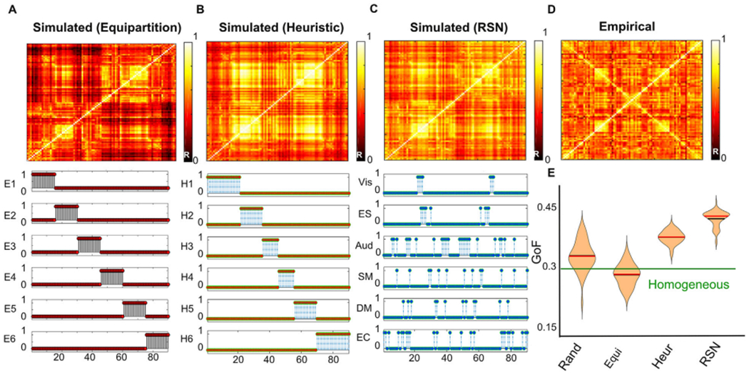
FC matrices obtained from the whole-brain model fitted to empirical FC using the equipartition prior (panel A), heuristic prior (panel B) and the RSN prior (panel C) present GoF value respectively GoF_W,E = 0.29, GoF_W,H = 0.38 and GoF_W,RSN = 0.43 comparing with the empirical FC matrix (panel D). The bottom part of all panels shows the indicator function 1_Gj (i) of Eq. (3), signaling the group membership of node i. The empirical FC matrix is displayed in panel D. As shown in panel E, the best TFF is obtained using the RSN prior, followed by the heuristic prior. Black and red horizontal lines indicate the mean and the median of the distribution. The horizontal green line stands for the best GoF obtained with the exhaustive homogeneous exploration.

In spite of the ad-hoc selection of groups in the equipartition prior and in the empirically-driven selection of groups (heuristic prior), grouping the nodes based on RSN membership resulted in the best GoF, as shown in Fig. 3E. It is important to note that allowing independent regional contributions to the bifurcation parameters improved the GoF beyond what would be expected from simply increasing the number of free parameters in the model. This is because, as shown in Fig. 3E, random and equipartition assignment of the coefficients to six groups yielded a GoF comparable to that of the model using the same bifurcation parameter for all nodes (homogeneous prior). The statistical comparison of the GoF for all pairs of priors is shown in Fig. S4 of the supplementary information.

The optimal parameters for wakefulness FC are shown in Fig. 4 for the heuristic (upper panel) and RSN (bottom panel) priors. The violin plots show the distribution of optimal coefficients across 100 independent optimizations, highlighting the convergence of the genetic algorithm. The parameters shown in Fig. 4 correspond to the coefficients that the nodes within each group contribute to the linear combination in Eq. (3). Thus, positive values (Vis and SM networks) indicate a contribution towards oscillatory dynamics at the limit cycle, while negative values (ES, Aud, DM, and EC networks) indicate a contribution towards noise-dominated dynamics at the fixed point. A replication with a larger number of independent optimization is shown in Fig. S5 for the RSN prior.

Fig. 4.

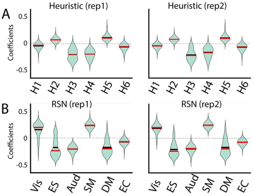
Coefficient distributions for 100 independent runs of the optimization procedures, for each group of nodes yielding the optimal GoF between simulated and empirical FC for the heuristic prior (panel A) and the RSN prior (panel B). Two sets (left and right) of 100 runs of optimization algorithm and are shown to highlight the convergence of the model parameters along repetitions (see Fig S5 to more repetitions). Black and red horizontal lines indicate the mean and the median of the distribution.

3.2. Changes in regional dynamics from wakefulness to deep sleep

Based on the results shown in Fig. 3E, we selected the RSNs as a canonical basis to constrain the independent parameters in our model. Next, we fitted the whole-brain model to the empirical FC obtained during wakefulness, N1, N2 and N3 sleep. The estimated parameters correspond to the coefficients that each node contributes to the linear combination yielding the final local bifurcation parameter.

The comparison of the optimal simulated FC matrices (average of 100 independent runs of the optimization procedure using the RSN prior) vs. the empirical FC is shown in Fig. 5. While for all stages the simulated intra-hemispheric FC resembled the empirical matrix, the issue of missing homotopic FC persisted during sleep and, for N3 sleep, the underestimation of inter-hemispheric FC extended to pairs of nonhomotopic regions. Fig. 5B shows simulated FC obtained after setting all homotopic weights (i.e. the contradiagonal) in SC to the maximum value of 0.2, following previous work by Deco and colleagues (Deco et al., 2014) and Messé and colleagues (Messé et al., 2014). As expected from these studies, this modification did not only improve the simulated homotopic FC, but also the overall GoF by inducing a higher similarity between simulated and empirical non-homotopic inter-hemispheric FC. This ad-hoc modification was performed to show how the limitations in SC computation affect the optimal GoF. In Fig. S6 of the supplementary information we show the optimal coefficients with and without the ad-hoc inclusion of contradiagonal SC weights.

Fig. 5.

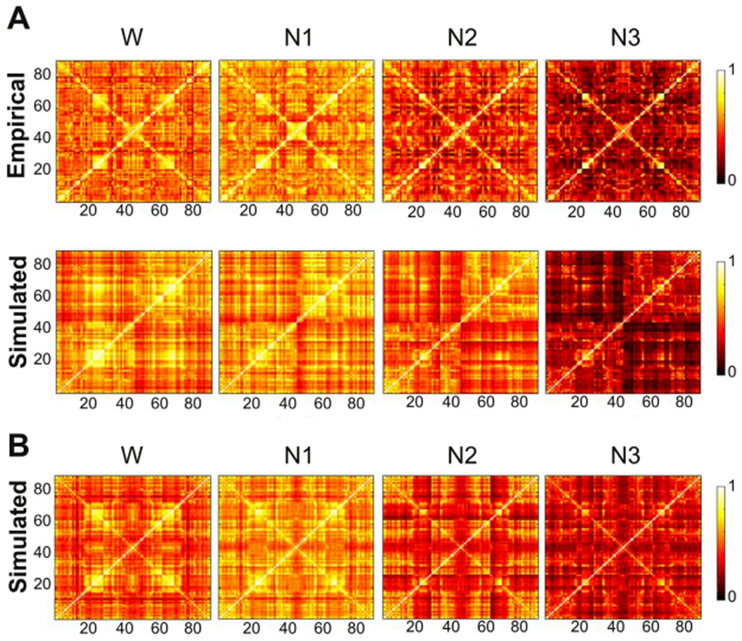
Comparison of empirical and simulated FC matrices for wakefulness and all sleep stages. A) Empirical and simulated FC, optimal fit using the RSN prior without changes to the SC. The obtained GoF between the empirical and simulated FC for each state are: GoF_W = 0.43, GoF_N1 = 0.41, GoF_N2 = 0.38and GoF_N3 = 0.33 B) Simulated FC matrices for wakefulness and all sleep stages with an ad-hoc increment in the homotopic SC. The values of GoF obtained are: GoF_W = 0.50, GoF_N1 = 0.48, GoF_N2 = 0.45and GoF_N3 = 0.42.

Fig. 6 shows the parameters corresponding to the optimal simulated FC matrices presented in Fig. 5A. The upper panels show violin plots for the distribution of the coefficients per RSN and sleep stage across 100 independent optimizations. The bottom panels present a comparison of these distributions for all pairs of stages in terms of Cohen’s d (d_Cohen). The Cohen’s d measures the effect size in terms of the difference between the means of two populations (μ_1,2) and the pooled standard deviations (s) as follows: $d=\frac{{\mu }_1-{\mu }_1}{s}$. We related Cohen’s d values to the effect size using a standard criterion (Sawilowsky, 2019): d_Cohen<0.2 is considered very low effect size, while d_Cohen>0.8 is considered very high effect size. Primary visual nodes (Vis network) contributed towards oscillatory dynamics during wakefulness, but this contribution progressively approached zero as the subjects transitioned towards N3 sleep. This appears reflected in the matrix containing the d_Cohen values, since the effect size is in the “very large” range (d_Cohen> 0.8) for the comparison of N3 vs. all stages. Results were similar for sensorimotor regions (SM network). Conversely, default mode regions (DM network) approached zero during sleep from negative coefficient values, i.e. local dynamics unfolded around a stable fixed-point during wakefulness, and approached the bifurcation progressively as the subjects transitioned towards N3 sleep. The remaining RSNs did not present clear trends, as their coefficients remained relatively stable around negative values (ES and Aud networks), or values very close to the bifurcation point (EC network).

Fig. 6.

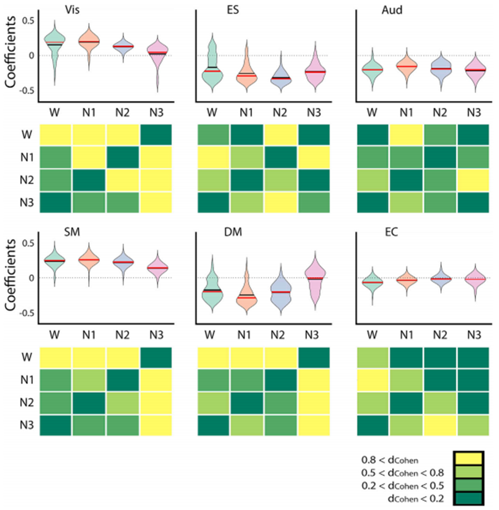
The coefficient distributions corresponding to the six RSNs, estimated from the optimal fit to the empirical FC data recorded during wakefulness (W), N1, N2 and N3 sleep. The bottom panels on each row show Cohen’s d (d_Cohen) for all pairwise comparisons. Primary visual (Vis) and sensorimotor (SM) nodes contributed towards oscillatory dynamics during wakefulness, but this contribution progressively approached zero as the subjects transitioned towards N3 sleep. The opposite result was observed for default mode (DM) nodes. In Fig S8, the coefficient distributions corresponding to the six RSNs were obtained for 100 runs of the optimization procedure with 20 individuals per generations.

Since the final regional bifurcation parameter of each node is obtained through linear combination of the coefficients of each group that node belongs to (Eq. (3)), for the nodes belonging to a single RSN their coefficients are equal to their final bifurcation parameters. However, this does not need to be the case for multiple RSN memberships. The differences in the final bifurcation parameters (wakefulness vs. N1, N2 and N3 sleep) are shown rendered into brain anatomy in Fig. 7. Sleep was modeled by a reduction in bifurcation parameter in nodes belonging to sensory and motor networks. The opposite result was observed for nodes belonging to parietal and frontal regions that can be included in the DMN. This result was also present for N2 and N3 sleep vs. wakefulness, with the addition of frontoparietal and temporal nodes becoming shifted from fixed point towards oscillatory dynamics.

Fig. 7.

Changes in regional bifurcation parameters during sleep relative to wakefulness. Rendering of the regions associated with very large effect sizes (d_Cohen> 0.8) in the comparison of the bifurcation parameters corresponding to sleep (N1, N2, and N3) vs. wakefulness. Red and blue regions indicate d_Cohen> 0.8 for wakefulness < sleep and wakefulness > sleep, respectively. This implies that sleep transitions the dynamics towards a≈0, i.e. dynamics become more susceptible to external perturbations.

3.3. Modeling the qualitative behavior of subcortical nodes during the wake-sleep transition

The onset of sleep is known to bring about changes in the activity and FC of subcortical nuclei, especially those located within the thalamus and hypothalamus (Magnin et al., 2010; Picchioni et al., 2014; Tagliazucchi and Laufs, 2014). The thalamus consists of a multitude of nuclei of neurons densely connected by reciprocal pathways with the cerebral cortex, which have multiple functions, including acting as a relay station between sensory systems and cortex (Sherman and Guillery, 1996). It has been speculated that changes in thalamic activity during sleep onset could be related to the need of isolating the brain from external arousing stimuli (Magnin et al., 2010). Thalamic deactivation precedes cortical deactivation, leading us to expect changes in the bifurcation parameters of subcortical nuclei during N1 sleep.

We extended the RSN prior to include an additional set of nodes corresponding to subcortical structures within the AAL atlas (thalamus, globus pallidus, putamen and caudate, all bilateral). It is interesting to note that since these structures are included in several RSNs, their co-efficients and the final bifurcation parameters need not necessarily be equal. Thus, adding these nodes as an independent group allowed us to test whether we could reproduce known neurophysiological changes that occur at the onset of sleep, and to evaluate whether parameters that are “hidden” within the model as part of the combination of variables determining the observable local dynamics can contain meaningful information.

The results of this analysis are presented in Fig. 8. The left panel shows the coefficients of the subcortical nodes as a function of sleep stage. It can be seen that the contribution of these nodes to the bifurcation parameter is consistently negative, with the largest negative value during N1 sleep. d_Cohen values for the comparison between all sleep stages confirm that N1 sleep presents subcortical coefficients different to those of wakefulness, N2 and N3 sleep. Since moving away from synchronized oscillatory dynamics is associated with decreased FC, this result is consistent with previous work showing that subcortical regions become deactivated and decoupled from the cortex during early sleep (Magnin et al., 2010; Picchioni et al., 2014; Tagliazucchi and Laufs, 2014). The right panel shows that this result is less evident in the bifurcation parameters, with the effect sizes becoming smaller and reaching >0.8 only for the comparison against N3 sleep. This suggests that information concerning the subcortical decoupling is more readily retrieved from hidden variables (coefficients) than from the bifurcation parameters, which are directly related to the observables produced by the model.

Fig. 8.

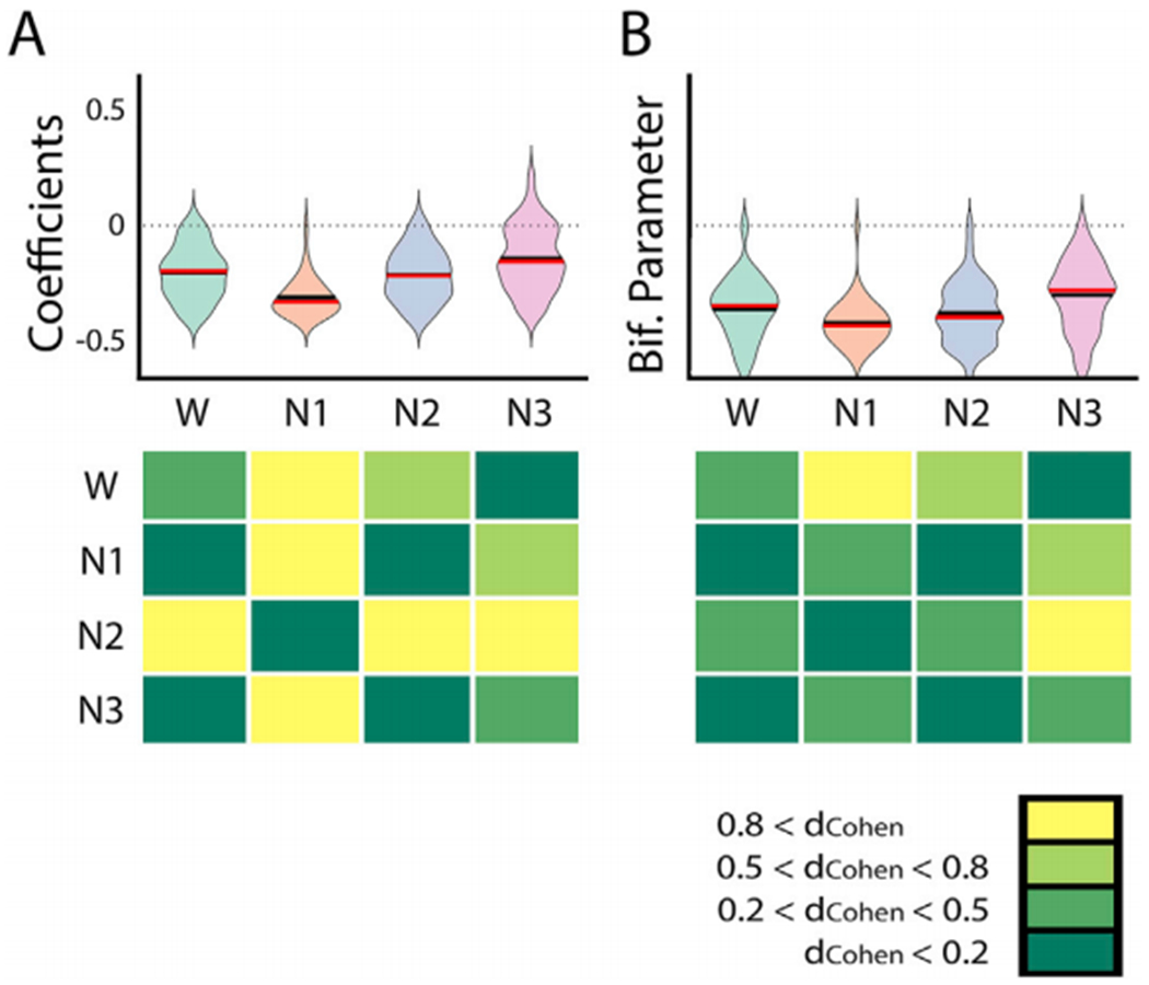
Changes in the coefficients (panel A) and bifurcation parameters (panel B) of subcortical nodes from wakefulness to deep sleep. The bottom panels show Cohen’s d (d_Cohen) for all pairwise comparisons.

3.4. Modeling externally induced transitions from deep sleep to wakefulness

An important justification for the development of computational models of whole-brain activity is the in silico rehearsal of invasive and non-invasive brain interventions (e.g. tACS). Exploratory computational analyses could help identify optimal external perturbations to induce transitions between brain states.

We modified our model to simulate external perturbations with the aim of inducing an arousal from the deepest sleep stage (N3) to wakefulness. Our simulated stimulation protocol was based on an additive oscillatory forcing applied to pairs of homotopic nodes using the natural frequency of those nodes to maximize the effect of the perturbation. We exhaustively explored the values of the forcing amplitude F₀ from 0 to 2 in steps of 0.05, applied to all 45 pairs of homotopic nodes. The capacity of the stimulation to induce transitions between states was assessed using the metric ΔGoF_norm (see Eq. (5)).

The qualitative behavior of ΔGoF_norm as a function of F₀ was heterogeneous and depended on the stimulated pair of nodes. We identified 10 pairs of nodes presenting ΔGoF_normvalues below 0.5 for at least one value of F₀; in other words, by stimulating each of these 10 pairs of nodes, the simulated FC was closer to that of wakefulness than to deep sleep.

Fig. 9 shows the behavior of these pairs of nodes against F₀. Nodes presented three different qualitative behaviors; these are indicated using different colors in the plot of ΔGoF_norm vs. F₀. In red, stimulation of the posterior cingulate cortex (PCC) monotonously decreased ΔGoF_norm up to 0.24. In green, the inferior occipital gyrus (IOG) reached a minimum ΔGoF_norm (0.31) for an intermediate F₀ value, and then remained approximately constant. Finally, the middle temporal gyrus (MTG, shown in blue) presented a clear global minimum of ΔGoF_norm (0.25) which then increased as a function of F₀.

Fig. 9.

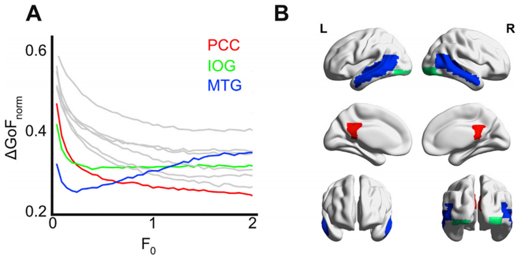
In silico stimulation of the model fitted to deep sleep using an additive oscillatory forcing term. A) ΔGoF_norm against the forcing amplitude F₀ for the 10 pairs of nodes leading to the lowest ΔGoF_norm values. B) Rendering of the three regions presenting the lowest ΔGoF_norm. The color code indicates three different qualitative behaviors as F₀ is increased: ΔGoF_norm decreases as a function of F₀ (posterior cingulate cortex [PCC], shown in red), ΔGoF_norm achieves an optimal value and then increases as a function of F₀ (middle temporal gyrus [MTG], shown in blue), and ΔGoF_norm remains approximately constant as a function of F₀ (inferior occipital gyrus [IOG], shown in green).

4. Discussion

The usefulness of both descriptive and computational models in neuroscience comes from a balance between complexity and interpretability. Models strive to reduce the intrinsic complexity of the human brain, producing interpretable explanations linking behavior, cognition and neurobiology. Computational models based on interpretable parameters can be used to study how empirical observables depend on these parameters in isolation of others of less interest, by means of the freedom granted by in silico exploration. Global brain states are frequently described and modeled in terms of their level of consciousness, thus increasing the ease of description at the expense of a very simplified unidimensional characterization. We developed and evaluated models of whole-brain activity with anatomically heterogeneous parameters, in line with the proposal for the multidimensional characterization of states of consciousness (Bayne et al., 2016, 2017), i.e. the proposal that independent factors must be considered for a full characterization of conscious states.

These models are built upon previous work using supercritical Hopf bifurcations to represent different regimes of local dynamics in fMRI data (Deco et al., 2017a, 2017b; Jobst et al., 2017, Donnelly-Kehoe et al., 2019). We expanded the parameter space to account for regional variations in the level of activation, interpreted as the capacity of a node to engage in sustained large amplitude synchronous activity. The functional segregation of the human brain into systems that are differentially activated during cognition is known since the earliest days of neurology, and this knowledge was greatly advanced by the introduction of non-invasive neuroimaging tools (Frackowiak, 2017). Due to this specialization, even if different brain states bring about global changes in brain metabolism, the functional consequences of these changes are likely to manifest regional dependence. Thus, we simulated FC for the different levels of arousal in the wake-deep sleep progression by introducing parameters representing the capacity of each chosen group of nodes to drive the local dynamics towards or away from the Hopf bifurcation.

Our approach was initially agnostic with regard to the grouping of the nodes within a six-dimensional parameter space. We determined that the RSN prior overperformed a grouping that heuristically captured the behavior of correlations in the empirical FC matrix, as well as an ad hoc grouping based on node equipartition. The relevance of the anatomical priors is evident from the observation that, regardless of incorporating five new independent parameters, the random assignment of nodes to the groups led to GoF similar to that obtained using the same parameter for all nodes (i.e. the homogeneous prior). This result represents a useful development in terms of model building, allowing multidimensional and mechanistic characterizations of global brain states beyond the intuition of “level of consciousness”. The dimensions of analysis are given by the choice of anatomical priors, and the mechanisms (in our case, differences in dynamical stability associated with changes in bifurcation parameters) can be explored by selecting different models for the local dynamics. The choices are not limited to RSNs and non-linear oscillators; for instance, an alternative can be found in recent work using serotonin receptor density maps to constrain the local gain in mean field models, and to investigate the mechanisms underlying the acute effects of a psychedelic compound (Deco et al., 2018b).

The simplifications of our computational model are justified by assumptions whose validity should be discussed before engaging in the interpretation of our findings. Oscillatory dynamics are ubiquitous in electrophysiological data, and reconfigurations of the power spectrum of collective neural oscillations are a landmark feature of transitions between different brain states (Steriade et al., 1993; Buzsaki, 2006). While fMRI is limited with respect to the identification of synchronous dynamics due to its comparatively low sampling rate, reliable reports of hemodynamic oscillations exist (obtained using ultrafast fMRI sequences [McAvoy et al., 2008; Baria et al., 2011]). These oscillations are likely of neural origin, since multimodal EEG-fMRI studies demonstrated their positive correlation with infra-slow (0.01–0.1 Hz) fluctuations in scalp potentials (Keinänen et al., 2018). More sophisticated models of mesoscopic brain activity, such as neural mass models, present several bifurcations including a supercritical Hopf from noisy to oscillatory dynamics (Grimbert and Faugeras, 2006; Coombes, 2010). By adopting the normal form of the bifurcation as a model, we made the further simplification of each node having a single dominant intrinsic oscillation frequency. Finally, our model neglects conduction delays since the temporal scale of fMRI oscillations is much slower than signal propagation times (Cabral et al., 2011). The validity of this simplification also depends on the temporal averaging of FC, since conduction delays could have an effect on the intermittency and lifespan of transient global synchronization patterns observed using fMRI.

The synergy between different empirical sources of data and our model for regional dynamics allows interpretation of the parameters beyond what could be inferred from fMRI data alone. For instance, while oscillatory dynamics in the fMRI signals could be assessed by directly computing the power spectrum from the data (Baria et al., 2011), our model allows to disentangle the intrinsic oscillatory dynamics of each region from synchronization arising due to collective effects (i.e. coupling between nodes with different degree of proximity to the bifurcation; see the example provided in Fig. 1). Furthermore, our proposed model includes hidden variables, the coefficientΔa_i, whose linear combination yields the bifurcation parameter, which is directly related to an empirical observable (the proximity to synchronous dynamics). However, as shown in Fig. 8 (left panel), these parameters can represent neurobiologically relevant results such as the known subcortical uncoupling and deactivation at sleep onset (Magnin et al., 2010), which can be obscured in terms of the bifurcation parameters (Fig. 8, right panel). This suggests that model fitting using individual fMRI and DTI data could yield new parameters with valuable contributions towards brain state discrimination, with potential applications in the training of machine learning models for neurological disease diagnosis and prognosis.

The regional distribution of the estimated bifurcation parameters pictures the division of the cortex into two different dynamical regimes along the progression from wakefulness to deep sleep. Sensory areas approached the bifurcation from oscillatory dynamics, while higher-level regions such as those in the DMN presented the opposite behavior. In terms of FC, these changes translated into decreased long-range correlations between the simulated time series, consistent with multiple reports of regionally decreased FC during sleep (Horovitz et al., 2009; Sämann et al., 2011; Tagliazucchi and Laufs, 2014; Tagliazucchi and Van Someren, 2017). Recent work by Song and colleagues showed that the onset of sleep increased the power of BOLD oscillations throughout widespread cortical and subcortical regions (Song et al., 2019). An interesting observation arising from our work is that sleep gives rise to a state of diminished FC and decreased activation in several regions. However, by virtue of increased proximity to the Hopf bifurcation, these changes also endow sleep with higher synchronizability, i.e. the latent capacity to react upon external perturbations. In this sense, our model captures the difference between an on-line activated state with ongoing stable frontoparietal dynamics (wakefulness), and an off-line deactivated state with reduced and noisy intrinsic dynamics in sensory regions, but frontoparietal dynamics highly reactive to environmental perturbations (sleep). Note that stability refers to proximity to the Hopf bifurcation. In terms of the dimensions of analysis suggested by Bayne and colleagues, this can be interpreted as increased global accessibility coexisting with reduced sensory gating.

We note that the interpretation of the model also depends on the metric chosen to determine the GoF. Previous studies used metrics related to FC dynamics and metastability (Hansen et al., 2015; Deco et al., 2017; Orio et al., 2018), capturing the statistical distribution of FC temporal fluctuations. However, the optimal fit in this sense is not necessarily the optimal fit in the sense of reproducing the temporally averaged FC. A similar argument applies to GoF metrics based on the mean and variance of the Kuramoto order parameter. Since our aim was to investigate how regional dynamics related to inter-areal coordination during different brain states, the use of a GoF metric based on the static FC matrices emerged as a natural choice. However, future studies could optimize local parameters in terms of observables related to the level of metastability. Also, future models based on non-equilibrium dynamics (e.g. chaotic oscillators) (Li and Chen, 2004; Orio et al., 2018) could be explored as means to simultaneously describe static FC and its temporal fluctuations.

We addressed the effect of external oscillatory perturbations, complementing previous modeling work using other perturbation protocols (Roberts and Robinson, 2012; Deco et al., 2017, 2018, 2019; Saenger et al., 2017). The choice of periodic forcing aims to capture the effects of tACS, one of the most currently used and researched protocols for non-invasive electrical stimulation. The use of nodal natural oscillatory frequency (inferred from fMRI data) in the additive forcing term can be justified by reports of electrophysiological oscillations being entrained by in-phase tACS stimulation (Helfrich et al., 2014), even though this mechanism has been recently disputed (Lafon et al., 2017). Simulated periodic forcing at pairs of homotopic regions informed potential mechanisms underlying arousal from deep sleep. Regions within sensory systems (i.e. temporal and occipital lobes) and the SC hub located at the posterior cingulate gyrus (Hagmann et al., 2018) presented the highest capacity to transition towards wakefulness. The relationship between forcing amplitude (F₀) and similarity to wakefulness (ΔGoF_norm) was complex and region-specific. Sensory regions showed an optimal ΔGoF_norm at an intermediate value, with saturation or even diminishing ΔGoF_norm for increasing F₀, consistent with results obtained using more biophysically realistic models by Ali and colleagues (Ali et al., 2013). In contrast, forcing at the posterior cingulate gyrus yielded a monotonously decreasing relationship between ΔGoF_norm and F₀. The rich connectivity of this node suggests that the effects of the forcing may depend on indirect connections reaching other critical regions through one or more intermediate steps. Considering this, it is critical that the development of non-invasive stimulation protocols to induce transitions between brain states is informed by computational models that explore the effects of combined stimulation at multiple brain regions. In the same way we used a genetic algorithm combined with anatomical priors for dimensionality reduction to optimize the TFF defined as 1-GoF, future studies could follow this method for the optimization of stimulation protocols to induce transitions. An important caveat is that the source current density resulting from tACS stimulation bears a complex relationship with the scalp position of the electrodes, since intermediate tissues can distort the currents and a considerable fraction of the current leaks through conductive non-neural tissue (Kasinadhuni et al., 2017). Thus, the in silico rehearsal of stimulation protocols cannot prescind of personalized models of current propagation (Huang et al., 2017).

In conclusion, we implemented a computational model synthesizing different sources of empirical data to achieve a mechanistic and multidimensional description of intermediate complexity of the different brain states visited during the progression from wakefulness to deep sleep. This model led us to a number of insights narrowing the space of possible dynamical mechanisms allowing the transition between self-organized brain states and their stabilization. We addressed the conceptual validation of our model by contrasting its predictions with known neurobiological results. As a relatively simple and interpretable model whose flexibility and specificity emerges from the incorporation of empirical information, we expect our developments will find applications in the multidimensional characterization of other brain states, and in the rehearsal of protocols to induce transitions between them.

References

- Donnelly-Kehoe P, Saenger VM, Lisofsky N, Kühn S, Kringelbach ML, Schwarzbach J, et al. , 2019. Reliable local dynamics in the brain across sessions are revealed by whole-brain modeling of resting state activity. Hum. Brain Mapp 10.1002/hbm.24572. [DOI] [PMC free article] [PubMed] [Google Scholar]
- Achard S, Salvador R, Whitcher B, Suckling J, Bullmore ED, 2006. Aresilient, low-frequency, small-world human brain functional network with highly connected association cortical hubs. J. Neurosci 26 (1), 63–72. [DOI] [PMC free article] [PubMed] [Google Scholar]
- Ali MM, Sellers KK, Fröhlich F, 2013. Transcranial alternating current stimulation modulates large-scale cortical network activity by network resonance. J. Neurosci 33 (27), 11262–11275. [DOI] [PMC free article] [PubMed] [Google Scholar]
- Allen PJ, Polizzi G, Krakow K, Fish DR, Lemieux L, 1998. Identification of EEG events in the MR scanner: the problem of pulse artifact and a method for its subtraction. Neuroimage 8 (3), 229–239. [DOI] [PubMed] [Google Scholar]
- Baker AP, Brookes MJ, Rezek IA, Smith SM, Behrens T, Smith PJP, Woolrich M, 2014. Fast transient networks in spontaneous human brain activity. Elife 3, e01867. [DOI] [PMC free article] [PubMed] [Google Scholar]
- Baria AT, Baliki MN, Parrish T, Apkarian AV, 2011. Anatomical and functional assemblies of brain BOLD oscillations. J. Neurosci 31 (21), 7910–7919. [DOI] [PMC free article] [PubMed] [Google Scholar]
- Bartolomei F, Naccache L, 2011. The global workspace (GW) theory of consciousness and epilepsy. Behav. Neurol 24 (1), 67–74. [DOI] [PMC free article] [PubMed] [Google Scholar]
- Bayne T, Hohwy J, Owen AM, 2016. Are there levels of consciousness? Trends Cognit. Sci 20 (6), 405–413. [DOI] [PubMed] [Google Scholar]
- Bayne T, Hohwy J, Owen AM, 2017. Reforming the taxonomy in disorders of consciousness. Ann. Neurol 82 (6), 866–872. [DOI] [PubMed] [Google Scholar]
- Beckmann CF, DeLuca M, Devlin JT, Smith SM, 2005. Investigations into resting-state connectivity using independent component analysis. Phil. Trans. Biol. Sci 360 (1457), 1001–1013. [DOI] [PMC free article] [PubMed] [Google Scholar]
- Behrens TE, Woolrich MW, Jenkinson M, Johansen-Berg H, Nunes RG, Clare S, Matthews PM, Brady JM, Smith SM, 2003. Characterization and propagation of uncertainty in diffusion-weightedMR imaging. Magn. Reson. Med 50, 1077–1088. [DOI] [PubMed] [Google Scholar]
- Behrens TE, Berg HJ, Jbabdi S, Rushworth MF, Woolrich MW, 2007. Probabilistic diffusion tractography with multiple fibre orientations: what can we gain? Neuroimage 34, 144–155. [DOI] [PMC free article] [PubMed] [Google Scholar]
- Berkovitch L, Dehaene S, Gaillard R, 2017. Disruption of conscious access in schizophrenia. Trends Cognit. Sci 21 (11), 878–892. [DOI] [PubMed] [Google Scholar]
- Berry RB, Brooks R, Gamaldo CE, Harding SM, Marcus CL, Vaughn BV, 2012. The AASM Manual for the Scoring of Sleep and Associated Events Rules, Terminology and Technical Specifications, Darien, Illinois, vol. 176 American Academy of Sleep Medicine. [Google Scholar]
- Biswal B, Zerrin Yetkin F, Haughton VM, Hyde JS, 1995. Functional connectivity in the motor cortex of resting human brain using echo-planar MRI. Magn. Reson. Med 34 (4), 537–541. [DOI] [PubMed] [Google Scholar]
- Breakspear M, 2017. Dynamic models of large-scale brain activity. Nat. Neurosci 20 (3), 340. [DOI] [PubMed] [Google Scholar]
- Buckner RL, Sepulcre J, Talukdar T, Krienen FM, Liu H, Hedden T, et al. , 2009. Cortical hubs revealed by intrinsic functional connectivity: mapping, assessment of stability, and relation to Alzheimer’s disease. J. Neurosci 29 (6), 1860–1873. [DOI] [PMC free article] [PubMed] [Google Scholar]
- Buzsaki G, 2006. Rhythms of the Brain. Oxford University Press. [Google Scholar]
- Cabral J, Hugues E, Sporns O, Deco G, 2011. Role of local network oscillations in resting-state functional connectivity. Neuroimage 57 (1), 130–139. [DOI] [PubMed] [Google Scholar]
- Coombes S, 2010. Large-scale neural dynamics: simple and complex. Neuroimage 52 (3), 731–739. [DOI] [PubMed] [Google Scholar]
- Cordes D, Haughton VM, Arfanakis K, Carew JD, Turski PA, Moritz CH, et al. , 2001. Frequencies contributing to functional connectivity in the cerebral cortex in “resting-state” data. Am. J. Neuroradiol 22 (7), 1326–1333. [PMC free article] [PubMed] [Google Scholar]
- Damoiseaux JS, Rombouts SARB, Barkhof F, Scheltens P, Stam CJ, Smith SM, Beckmann CF, 2006. Consistent resting-state networks across healthy subjects. Proc. Natl. Acad. Sci. Unit. States Am 103 (37), 13848–13853. [DOI] [PMC free article] [PubMed] [Google Scholar]
- Deco G, McIntosh AR, Shen K, Hutchison RM, Menon RS, Everling S, et al. , 2014. Identification of optimal structural connectivity using functional connectivity and neural modeling. J. Neurosci. 34 (23), 7910–7916. [DOI] [PMC free article] [PubMed] [Google Scholar]
- Deco G, Kringelbach ML, Jirsa VK, Ritter P, 2017a. The dynamics of resting fluctuations in the brain: metastability and its dynamical cortical core. Sci. Rep 7 (1), 3095. [DOI] [PMC free article] [PubMed] [Google Scholar]
- Deco G, Tagliazucchi E, Laufs H, Sanjuán A, Kringelbach ML, 2017b. Novel intrinsic ignition method measuring local-global integration characterizes wakefulness and deep sleep. Eneuro 4 (5). [DOI] [PMC free article] [PubMed] [Google Scholar]
- Deco G, Cabral J, Saenger VM, Boly M, Tagliazucchi E, Laufs H, et al. , 2018a. Perturbation of whole-brain dynamics in silico reveals mechanistic differences between brain states. Neuroimage 169, 46–56. [DOI] [PubMed] [Google Scholar]
- Deco G, Cruzat J, Cabral J, Knudsen GM, Carhart-Harris RL, Whybrow PC, et al. , 2018b. Whole-brain multimodal neuroimaging model using serotonin receptor maps explains non-linear functional effects of LSD. Curr. Biol 28 (19), 3065–3074. [DOI] [PubMed] [Google Scholar]
- Deco G, Cruzat J, Cabral J, Tagliazucchi E, Laufs H, Logothetis NK, Kringelbach ML, 2019. Awakening: predicting external stimulation to force transitions between different brain states. Proc. Natl. Acad. Sci. Unit. States Am 116 (36), 18088–18097. [DOI] [PMC free article] [PubMed] [Google Scholar]
- Dehaene S, Naccache L, 2001. Towards a cognitive neuroscience of consciousness: basic evidence and a workspace framework. Cognition 79 (1–2), 1–37. [DOI] [PubMed] [Google Scholar]
- Frackowiak RS, 2017. The functional architecture of the brain In: The Brain. Routledge, pp. 105–130. [Google Scholar]
- Friston KJ, Williams S, Howard R, Frackowiak RS, Turner R, 1996. Movement-related effects in fMRI time-series. Magn. Reson. Med 35 (3), 346–355. [DOI] [PubMed] [Google Scholar]
- Fukushima M, Sporns O, 2018. Comparison of fluctuations in global network topology of modeled and empirical brain functional connectivity. PLoS Comput. Biol 14 (9), e1006497. [DOI] [PMC free article] [PubMed] [Google Scholar]
- Ghosh A, Rho Y, McIntosh AR, Kötter R, Jirsa VK, 2008. Noise during rest enables the exploration of the brain’s dynamic repertoire. PLoS Comput. Biol 4 (10), e1000196. [DOI] [PMC free article] [PubMed] [Google Scholar]
- Glerean E, Salmi J, Lahnakoski JM, Jääskeläinen IP, Sams M, 2012. Functional magnetic resonance imaging phase synchronization as a measure of dynamic functional connectivity. Brain Connect. 2 (2), 91–101. [DOI] [PMC free article] [PubMed] [Google Scholar]
- Glover GH, Li TQ, Ress D, 2000. Image-based method for retrospective correction of physiological motion effects in fMRI: RETROICOR. Magn. Reson. Med 44 (1), 162–167. [DOI] [PubMed] [Google Scholar]
- Greicius MD, Supekar K, Menon V, Dougherty RF, 2009. Resting-state functional connectivity reflects structural connectivity in the default mode network. Cerebr. Cortex 19 (1), 72–78. [DOI] [PMC free article] [PubMed] [Google Scholar]
- Grimbert F, Faugeras O, 2006. Bifurcation analysis of Jansen’s neural mass model. Neural Comput. 18 (12), 3052–3068. [DOI] [PubMed] [Google Scholar]
- Hagmann P, Cammoun L, Gigandet X, Meuli R, Honey CJ, Wedeen VJ, Sporns O, 2008. Mapping the structural core of human cerebral cortex. PLoS Biol. 6 (7), e159. [DOI] [PMC free article] [PubMed] [Google Scholar]
- Haimovici A, Tagliazucchi E, Balenzuela P, Chialvo DR, 2013. Brain organization into resting state networks emerges at criticality on a model of the human connectome. Phys. Rev. Lett 11 (17), 178101. [DOI] [PubMed] [Google Scholar]
- Hansen EC, Battaglia D, Spiegler A, Deco G, Jirsa VK, 2015. Functional connectivity dynamics: modeling the switching behavior of the resting state. Neuroimage 105, 525–535. [DOI] [PubMed] [Google Scholar]
- Helfrich RF, Schneider TR, Rach S, Trautmann-Lengsfeld SA, Engel AK, Herrmann CS, 2014. Entrainment of brain oscillations by transcranial alternating current stimulation. Curr. Biol 24 (3), 333–339. [DOI] [PubMed] [Google Scholar]
- Hobson JA, Pace-Schott EF, 2002. The cognitive neuroscience of sleep: neuronal systems, consciousness and learning. Nat. Rev. Neurosci 3 (9), 679–693. [DOI] [PubMed] [Google Scholar]
- Honey CJ, Kötter R, Breakspear M, Sporns O, 2007. Network structure of cerebral cortex shapes functional connectivity on multiple time scales. Proc. Natl. Acad. Sci. Unit. States Am 104 (24), 10240–10245. [DOI] [PMC free article] [PubMed] [Google Scholar]
- Honey CJ, Sporns O, Cammoun L, Gigandet X, Thiran JP, Meuli R, Hagmann P, 2009. Predicting human resting-state functional connectivity from structural connectivity. Proc. Natl. Acad. Sci. Unit. States Am 106 (6), 2035–2040. [DOI] [PMC free article] [PubMed] [Google Scholar]
- Horovitz SG, Braun AR, Carr WS, Picchioni D, Balkin TJ, Fukunaga M, Duyn JH, 2009. Decoupling of the brain’s default mode network during deep sleep. Proc. Natl. Acad. Sci. Unit. States Am 106 (27), 11376–11381. [DOI] [PMC free article] [PubMed] [Google Scholar]
- Huang Y, Liu AA, Lafon B, Friedman D, Dayan M, Wang X, et al. , 2017. Measurements and models of electric fields in the in vivo human brain during transcranial electric stimulation. Elife 6, e18834. [DOI] [PMC free article] [PubMed] [Google Scholar]
- Jenkinson M, Bannister P, Brady M, Smith S, 2002. Improved optimization for the robust and accurate linear registration and motion correction of brain images. Neuroimage 17 (2), 825–841. [DOI] [PubMed] [Google Scholar]
- Jobst BM, Hindriks R, Laufs H, Tagliazucchi E, Hahn G, Ponce-Alvarez A, et al. , 2017. Increased stability and breakdown of brain effective connectivity during slow-wave sleep: mechanistic insights from whole-brain computational modelling. Sci. Rep 7 (1), 4634. [DOI] [PMC free article] [PubMed] [Google Scholar]
- Kasinadhuni AK, Indahlastari A, Chauhan M, Schäor M, Mareci TH, Sadleir RJ, 2017. Imaging of current flow in the human head during transcranial electrical therapy. Brain Stimulat. 10 (4), 764–772. [DOI] [PMC free article] [PubMed] [Google Scholar]
- Keinänen T, Rytky S, Korhonen V, Huotari N, Nikkinen J, Tervonen O, et al. , 2018. Fluctuations of the EEG-fMRI correlation reflect intrinsic strength of functional connectivity in default mode network. J. Neurosci. Res 96 (10), 1689–1698. [DOI] [PubMed] [Google Scholar]
- Lafon B, Henin S, Huang Y, Friedman D, Melloni L, Thesen T, et al. , 2017. Low frequency transcranial electrical stimulation does not entrain sleep rhythms measured by human intracranial recordings. Nat. Commun 8 (1), 1199. [DOI] [PMC free article] [PubMed] [Google Scholar]
- Li C, Chen G, 2004. Phase synchronization in small-world networks of chaotic oscillators. Phys. Stat. Mech. Appl 341, 73–79. [Google Scholar]
- Lord LD, Expert P, Atasoy S, Roseman L, Rapuano K, Lambiotte R, et al. , 2019. Dynamical exploration of the repertoire of brain networks at rest is modulated by psilocybin. Neuroimage 199, 127–142. [DOI] [PubMed] [Google Scholar]
- Magnin M, Rey M, Bastuji H, Guillemant P, Mauguière F, Garcia-Larrea L, 2010. Thalamic deactivation at sleep onset precedes that of the cerebral cortex in humans. Proc. Natl. Acad. Sci. Unit. States Am 107 (8), 3829–3833. [DOI] [PMC free article] [PubMed] [Google Scholar]
- McAvoy M, Larson-Prior L, Nolan TS, Vaishnavi SN, Raichle ME, d’Avossa G, 2008. Resting states affect spontaneous BOLD oscillations in sensory and paralimbic cortex. J. Neurophysiol 100 (2), 922–931. [DOI] [PMC free article] [PubMed] [Google Scholar]
- Messé A, Rudrauf D, Benali H, Marrelec G, 2014. Relating structure and function in the human brain: relative contributions of anatomy, stationary dynamics, and non-stationarities. PLoS Comput. Biol 10 (3), e1003530. [DOI] [PMC free article] [PubMed] [Google Scholar]
- Opitz A, Yeagle E, Thielscher A, Schroeder C, Mehta AD, Milham MP, 2018. On the importance of precise electrode placement for targeted transcranial electric stimulation. Neuroimage 181, 560–567. [DOI] [PMC free article] [PubMed] [Google Scholar]
- Orio P, Gatica M, Herzog R, Maidana JP, Castro S, Xu K, 2018. Chaos versus noise as drivers of multistability in neural networks. Chaos: Interdiscipl. J. Nonlinear Sci 28 (10), 106321. [DOI] [PubMed] [Google Scholar]
- Picchioni D, Pixa ML, Fukunaga M, Carr WS, Horovitz SG, Braun AR, Duyn JH, 2014. Decreased connectivity between the thalamus and the neocortex during human nonrapid eye movement sleep. Sleep 37 (2), 387–397. [DOI] [PMC free article] [PubMed] [Google Scholar]
- Reveley C, Seth AK, Pierpaoli C, Silva AC, Yu D, Saunders RC, et al. , 2015. Superficial white matter fiber systems impede detection of long-range cortical connections in diffusion MR tractography. Proc. Natl. Acad. Sci. Unit. States Am 112 (21), E2820–E2828. [DOI] [PMC free article] [PubMed] [Google Scholar]
- Roberts JA, Robinson PA, 2012. Quantitative theory of driven nonlinear brain dynamics. Neuroimage 62 (3), 1947–1955. [DOI] [PubMed] [Google Scholar]
- Roberts JA, Gollo LL, Abeysuriya RG, Roberts G, Mitchell PB, Woolrich MW, Breakspear M, 2019. Metastable brain waves. Nat. Commun 10 (1), 1056. [DOI] [PMC free article] [PubMed] [Google Scholar]
- Rosow C, Manberg PJ, 2001. Bispectral index monitoring. Anesthesiol. Clin 19 (4), 947–966. [DOI] [PubMed] [Google Scholar]
- Saenger VM, Kahan J, Foltynie T, Friston K, Aziz TZ, Green AL, et al. , 2017. Uncovering the underlying mechanisms and whole-brain dynamics of deep brain stimulation for Parkinson’s disease. Sci. Rep 7 (1), 9882. [DOI] [PMC free article] [PubMed] [Google Scholar]
- Sämann PG, Wehrle R, Hoehn D, Spoormaker VI, Peters H, Tully C, et al. , 2011. Development of the brain’s default mode network from wakefulness to slow wave sleep. Cerebr. Cortex 21 (9), 2082–2093. [DOI] [PubMed] [Google Scholar]
- Sanz-Leon P, Knock SA, Spiegler A, Jirsa VK, 2015. Mathematical framework for large-scale brain network modeling in the Virtual Brain. Neuroimage 111, 385–430. [DOI] [PubMed] [Google Scholar]
- Sawilowsky SS, 2009. New effect size rules of thumb. J. Mod. Appl. Stat. Methods 8 (2), 26. [Google Scholar]
- Sergent C, Dehaene S, 2004. Neural processes underlying conscious perception: experimental findings and a global neuronal workspace framework. J. Physiol. Paris 98 (4–6), 374–384. [DOI] [PubMed] [Google Scholar]
- Sherman SM, Guillery RW, 1996. Functional organization of thalamocortical relays. J. Neurophysiol 76 (3), 1367–1395. [DOI] [PubMed] [Google Scholar]
- Song C, Tagliazucchi E, 2019. Linking the nature and functions of sleep: insights from multimodal imaging of the sleeping brain. Curr. Opin. Physiol 15, 29–36. 10.1016/j.cophys.2019.11.012. [DOI] [PMC free article] [PubMed] [Google Scholar]
- Song C, Boly M, Tagliazucchi E, Laufs H, Tononi G, 2019. BOLD Signatures of Sleep, p. 531186 bioRxiv. [DOI] [PMC free article] [PubMed] [Google Scholar]
- Spiegler A, Hansen EC, Bernard C, McIntosh AR, Jirsa VK, 2016. Selective activation of resting-state networks following focal stimulation in a connectome-based network model of the human brain. eNeuro 3 (5). [DOI] [PMC free article] [PubMed] [Google Scholar]
- Sporns O, Tononi G, Kötter R, 2005. The human connectome: a structural description of the human brain. PLoS Comput. Biol 1 (4), e42. [DOI] [PMC free article] [PubMed] [Google Scholar]
- Steriade M, McCormick DA, Sejnowski TJ, 1993. Thalamocortical oscillations in the sleeping and aroused brain. Science 262 (5134), 679–685. [DOI] [PubMed] [Google Scholar]
- Sternbach GL, 2000. The Glasgow coma scale. J. Emerg. Med 19 (1), 67–71. [DOI] [PubMed] [Google Scholar]
- Tagliazucchi E, Laufs H, 2014. Decoding wakefulness levels from typical fMRI resting-state data reveals reliable drifts between wakefulness and sleep. Neuron 82 (3), 695–708. [DOI] [PubMed] [Google Scholar]
- Tagliazucchi E, van Someren EJ, 2017. The large-scale functional connectivity correlates of consciousness and arousal during the healthy and pathological human sleep cycle. Neuroimage 160, 55–72. [DOI] [PubMed] [Google Scholar]
- Tagliazucchi E, von Wegner F, Morzelewski A, Borisov S, Jahnke K, Laufs H, 2012. Automatic sleep staging using fMRI functional connectivity data. Neuroimage 63 (1), 63–72. [DOI] [PubMed] [Google Scholar]
- Tart CT, 1972. States of consciousness and state-specific sciences. Science 176 (4040), 1203–1210. [DOI] [PubMed] [Google Scholar]
- Tassi P, Muzet A, 2001. Defining the states of consciousness. Neurosci. Biobehav. Rev 25 (2), 175–191. [DOI] [PubMed] [Google Scholar]
- Taylor PN, Wang Y, Goodfellow M, Dauwels J, Moeller F, Stephani U, Baier G, 2014. A computational study of stimulus driven epileptic seizure abatement. PloS One 9 (12), e114316. [DOI] [PMC free article] [PubMed] [Google Scholar]
- Tononi G, Edelman GM, 1998. Consciousness and complexity. Science 282 (5395), 1846–1851. [DOI] [PubMed] [Google Scholar]
- Treisman A, 1998. Feature binding, attention and object perception. Phil. Trans. Roy. Soc. Lond. B Biol. Sci 353 (1373), 1295–1306. [DOI] [PMC free article] [PubMed] [Google Scholar]
- Tzourio-Mazoyer N, Landeau B, Papathanassiou D, Crivello F, Etard O, Delcroix N, et al. , 2002. Automated anatomical labeling of activations in SPM using a macroscopic anatomical parcellation of the MNI MRI single-subject brain. Neuroimage 15 (1), 273–289. [DOI] [PubMed] [Google Scholar]
- Van Den Heuvel MP, Mandl RC, Kahn RS, Hulshoff Pol HE, 2009. Functionally linked resting-state networks reflect the underlying structural connectivity architecture of the human brain. Hum. Brain Mapp 30 (10), 3127–3141. [DOI] [PMC free article] [PubMed] [Google Scholar]
- Vidaurre D, Abeysuriya R, Becker R, Quinn AJ, Alfaro-Almagro F, Smith SM, Woolrich MW, 2018. Discovering dynamic brain networks from big data in rest and task. Neuroimage 180, 646–656. [DOI] [PMC free article] [PubMed] [Google Scholar]
- Wang Z, Bovik AC, Sheikh HR, Simoncelli EP, 2004. Image quality assessment: from error visibility to structural similarity. IEEE Trans. Image Process 13 (4), 600–612. [DOI] [PubMed] [Google Scholar]
- Windt JM, Nielsen T, Thompson E, 2016. Does consciousness disappear in dreamless sleep? Trends Cognit. Sci 20 (12), 871–882. [DOI] [PubMed] [Google Scholar]
- Zhou W, Bovik AC, Sheikh HR, Simoncelli EP, April 2004. Image qualifty assessment: from error visibility to structural similarity. IEEE Trans. Image Process 13 (Issue 4), 600–612. [DOI] [PubMed] [Google Scholar]
Associated Data
This section collects any data citations, data availability statements, or supplementary materials included in this article.