Abstract
We examine the influence of shear anisotropy of brain tissue on the potential for mild traumatic brain injury. First we develop a new constitutive description for the white matter in the brain that can capture the anisotropic behavior of the white matter in both tension and shear. The material parameters for the models are determined using a set of three experiments already published in the literature. The calibrated and parameterized model is then implemented in a computational (finite element) model of the head. This computational model is two-dimensional and is used to simulate a previously published injury-causing event in the National Hockey League, using axonal strain as criterion to assess the level of diffuse axonal injury. It is demonstrated that the inclusion of shear anisotropy affects both the nature and the extent of predicted injury. Further, the locations of the predicted injury are more consistent with observations in the literature.
Keywords: Shear anisotropy, Constitutive-model, TBI, Injury
INTRODUCTION
Traumatic Brain Injury (TBI)1 is typically caused by a sudden mechanical loading to the head such as that resulting from a fall, a blast or a car crash. The level of injury is classified as mild, moderate or severe depending on the degree and nature of damage to the brain. More than 82% of military TBI in the years 2000–2017 were mild, and hence greater efforts are typically focused towards mild TBI (mTBI).8 It is difficult to properly diagnose mTBI and the corresponding damage in the brain at the acute stages of injury, due to a lack of abnormalities in standard medical imaging immediately after an mTBI-causing event. In this context, computational simulations offer some hope for both understanding and early diagnosis of mTBI.
Finite element models are often used as computational tools to study mTBI and estimate injury in humans. These models are either two dimensional (2D)31,42,43 or three dimensional (3D) models,3,5,11,29,30,39,45 and differ greatly in the anatomical details that are considered, ranging from low to high fidelity.
Most early TBI computations treated brain tissue as isotropic material.9,17,36,45,47 With the discovery of the brain’s fiber network, some TBI models have used anisotropic descriptions for the white matter and isotropic descriptions to represent gray matter.37,42,43 The anisotropic models have been developed by using both continuum(e.g. Ref. 26) or structural (e.g. Ref. 19) approaches. However, all of the TBI models to date have accounted for anisotropy in tension but not in shear, despite clear evidence of shear anisotropy in white matter.13
In this work we present a material model for white matter that captures anisotropy in both tension and shear. The material parameters are determined by calibration with respect to data from the literature and the calibrated model is then validated against live human data in a non-injurious context. The validated model is then used to simulate a specific National Hockey League (NHL) incident that resulted in injury. In order to demonstrate the role of shear anisotropy in mTBI modelling, the results of the new material model are compared to the results obtained with model that includes only tension anisotropy.
MATERIALS AND METHODS
The materials in brain tissue are typically separated into two types: white matter and gray matter. The gray matter primarily consists of neuronal cell bodies and is typically modeled as an isotropic material. On the other hand, the white matter is largely composed of axons surrounded by various types of glial cells forming a network of fiber bundles. The existence of this network causes the material to have a different response if stretched parallel to the fiber direction than if stretched perpendicular to the fiber direction.37 A similar anisotropy applies to the shear response.13 Thus, white matter is an anisotropic material in both tension and shear. In this section, a constitutive model for white matter is described which includes both modes of anisotropy.
Constitutive Model
We start with a simple volume of material with fibers in one direction. The initial fiber direction a0 in the reference configuration and the new fiber vector a in the deformed configuration are related through the deformation gradient F and the fiber stretch λ by
| (1) |
The strain energy function for a transversely isotropic material is usually represented using three invariants for the isotropic response of the material,
| (2) |
and two pseudo-invariants for the anisotropic response33
| (3) |
where C is the Right Cauchy–Green tensor. Note while I4 depends only on the fiber stretch, I5 carries information about both fiber stretch and fiber-matrix interaction.12 Since white matter is a nearly incompressible material and the model will be used in a finite element computation, the strain energy function is assumed to be partitioned to avoid shear locking, so that
| (4) |
where WVolumetric is the strain energy part allowing volume change and WIsochoric captures deformation without any change in volume. The deformation gradient tensor F is modified to
| (5) |
where J = detF is the volume ratio (WVolumetric = f(J)) and is the deformation gradient with constant volume . Accordingly the invariants are expressed in terms of the modified Cauchy–Green tensor . We now assume that the isochoric strain energy, WIsochoric, is composed of two parts, one representing the isotropic response of white matter (assumed to be Neo-Hookean) and the other representing the fiber reinforcement:
| (6a) |
| (6b) |
| (6c) |
where C1, C2 and C3 are material parameters. The WAnisotropic incorporates anisotropy in both tension and shear, and and are defined analogously to I1, I4 and I5 when F is replaced by . Note that the second term in Eq. (6c) represents the fiber-matrix interaction only. The values of the material parameters C1, C2 and C3 can be determined (e.g.) from three experiments:
Tension perpendicular to the fibers to obtain C1 since this mode is dominated by the matrix response to deformation.
Tension along the fiber direction to obtain C2 (mode dominated by the fiber stretch contribution).
Shear perpendicular to the fibers to obtain C3 (mode dominated by the fiber-matrix shear interaction).
We note that, to our knowledge, previous mTBI anisotropic white matter models have not accounted for the fiber-matrix interactions and I5 in the formulation.
Finally, the volumetric part of the strain energy is described in terms of the volume ratio J and the bulk modulus K, as is widely used in other studies for white matter4,5,11
| (7) |
With these definitions of the strain energy, the constitutive equation of white matter can be derived following12 with the Cauchy stress tensor σ related to the strain energy density by
| (8) |
where I is the identity tensor and is the modified Left Cauchy–Green tensor.
To understand the effects of the shear anisotropy (I5), we compare our results to those obtained using an anisotropic model without shear anisotropy: the Holzapfel–Gasser–Ogden (HGO) model which was used by Wright et al.42 For a single family of fibers in a representative volume, the HGO model used by Ref. 42 was:
| (9) |
where , k1 is a parameter representing tension anisotropy, k2 is a scaling factor and k is the fiber dispersion parameter. Note that the special case of k = 0 and a single fiber family and for small k2 (as in Wright et al.42), Eq. (9) reduces to the same form as Eq. (6) with C3 = 0 (i.e., only the ). The major difference between our model (Eq. 6) and the HGO model (Eq. 9) is the following: our model accounts for tension and shear anisotropy but fiber dispersion is not included, while the HGO model accounts for tension anisotropy and includes fiber dispersion but no shear anisotropy. Both models include fiber-induced anisotropy, but the HGO model allows the fiber directions to vary somewhat (depending on the dispersion).
Material Properties
Now that we have defined the constitutive models, we need to determine the parameters C1, C2 and C3 of Eq. (6), k1, k2 and k of Eq. (9) and the bulk modulus K of Eq. (7). Parameters for Eq. (9) were taken directly from Wright et al.42 (Table 1). The bulk modulus K is chosen to be 2.19 GPa, consistent with some (but by no means all) of the prior literature for TBI computations.34,40,44
TABLE 1.
Values for the material parameters in the shear anisotropic model (Eq. 6) determined by fitting the results of Velrdi et al.37 and Jin et al.,13 and in the HGO model (Eq. 9) used by Wright et al.42
| Shear anisotropic model | HGO model | |
|---|---|---|
| C1 (Pa) | 148 | 3200 |
| C2 (Pa) | 61 | – |
| C3 (Pa) | 505 | – |
| k1 (Pa) | – | 2716 |
| k2 | – | 0.0001 |
| k | – | From DTI(0 – 1/3) |
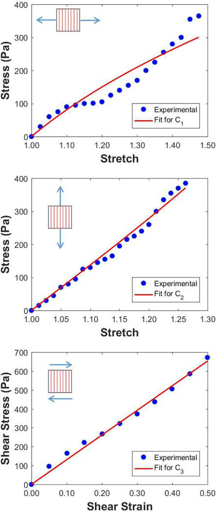
Since we expect the brain tissue to be strain-rate dependent,2,10,35 we incorporate viscoelastic effects through a Prony series (described in the next subsection). For this particular implementation, C1, C2 and C3 should be determined from low strain rate data of tension and shear experiments performed with respect to the dominant fiber direction, and there are few studies that have this information. Jin et al.13 examined tissues from four regions of human adult brains: Cortex, Thalamus, Corpus Callosum and Corona Radiata. Compression, tension and shear tests with respect to fiber direction were performed for all four regions using three strain rates (0.5, 5 and 30 s−1). An attempt to fit all the material parameters to the 0.5 s−1 strain rate data (lowest strain rate in Jin’s et al.13 dataset) results in a negative value for C3, which is not allowed in this hyperelastic model. It is possible that there are variations in the experimental data because of effects such as the long post-mortem time of the samples (averaging 4 days post mortem) or the fact that each test direction was performed on a different subject (gender and age differed, the latter ranging from 48 to 94 years). The net result is that we can not use the three tests of the low strain rate (0.5 s−1) in Jin’s et al.13 experiment to determine the full set of C1, C2 and C3. Instead we consider Velardi et al’s.37 work. They performed tensile tests on fresh adult porcine brain tissue from three different regions: Cortex, Corpus Callosum (CC) and Corona Radiata (CR) at a strain rate of 0.1 s−1. For both CC and CR, tension tests were performed both parallel and perpendicular to the fibers allowing us to obtain C1 and C2 [Fig. 1 (top and middle, respectively)]. However, Velardi et al.37 did not perform shear testing with respect to the fiber direction. To obtain C3, therefore, we used the work of Jin et al.13 The parameter C3 is determined by fitting the Jin et al.13 results for shear perpendicular to the fiber direction [Fig. 1 (bottom)]. A nonlinear least squares method was used for all parameters, which are shown in Table 1, and the corresponding R2 values are above 0.9 for the three parameters. Since both experimental studies13,37 we used for the fitting are performed under low strain rate loading (0.1 and 0.5 s−1 respectively), we consider the fitted parameters to define the long-term response of the material. The viscoelastic modulus behavior will be described in the next subsection.
FIGURE 1.
Determination of the material parameters for the shear anisotropic model (Eq. 6). The first Piola–Kirchhoff (PK) stress is plotted vs. the corresponding stretch (top and middle), and vs. the shear strain (bottom). The experimental measurements are taken from the work of Velardi et al.37 and Jin et al.13 The fits allow us to obtain C1 (top), C2 (middle) and C3 (bottom). Note: the relationship between the 1st PK stress (P) and the Cauchy stress σ (Eq. 8) is Jσ = FPT.
Given the availability of data, we have had to mix two tissue sources (porcine and human) when obtaining our parameters. Prange and Margulies27 compared the properties of porcine and human brain tissue, and found that human brain tissue was stiffer than the porcine tissue. On the other hand, Nicolle et al.25 obtained shear viscoelastic material properties for porcine tissue, compared them to human tissue properties reported in the literature, and concluded that porcine tissue stiffnesses were within the range of human tissue stiffnesses. Similarly, Nicolle et al.24 found no difference in the material properties of the brain tissue between the two species. In this context of the data in the available literature, we believe that using two different tissue sources to calibrate our model is reasonable.
Finite Element Head Model
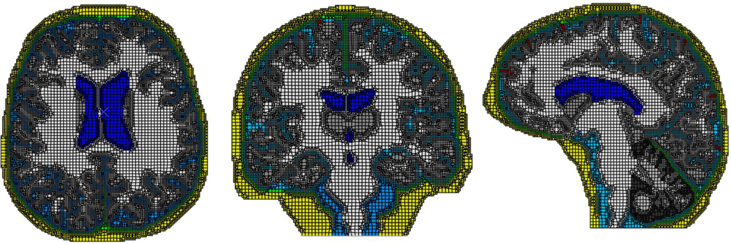
Our finite element (FE) head model is based on magnetic resonance image (MRI) data of a healthy human.42 For simplicity, and to provide insights into when building and running a more realistic but much more expensive 3D simulation is necessary (such simulations are underway), we consider three 2D slices (extracted from the 3D MRI), one for each plane: axial, coronal and sagittal. Each slice is segmented for the following brain structures when appropriate: skull, dura (with falx and tentorium), cerebro-spinal fluid (CSF), gray matter, white matter, cerebellum, bridging veins and ventricles (Fig. 2).
FIGURE 2.
The 2D finite element head models from the three representative planes: Axial (left), Coronal (middle) and Sagittal (right). The models include multiple brain structures that have been segmented from the MRI data.
The shear anisotropic model described in the previous section is used for white matter, with the primary fiber bundle direction assigned by co-registering the MRI with Diffusion Tensor Imaging (DTI) of the same subject, with the dominant direction of the fiber bundle for each voxel recorded. Since gray matter does not have a preferred orientation, we used Eq. (9) with the fiber dispersion k set to 1/3 for gray matter. Since the brain tissue mechanical behavior is dependent on the strain rate,7,10,28,35 we adapted a one-term Prony series shear modulus to compensate for the strain rate effect from Wright et al.42 The calibrated shear modulus (2C1) is considered as the long-term shear modulus, and using a commonly reported ratio long-term and short-term moduli42,46 the value of the long-term modulus is extracted. Table 2 summarizes the material models for all other structures.
TABLE 2.
Material models used for the head structures other than white matter.
| Material | Model | Equation |
|---|---|---|
| Cerebellum | NeoHookean | |
| Cerebrum and cerebellum | Viscoelastic | |
| Skull and dura | Linear elastic | |
| Bridging veins | 1st-order Ogden | |
| CSF | Mie-Gruneisen EOS |
The viscoelastic model is a one term Prony series defining the long-term and short-term shear moduli ( and respectively) and the decay constant β. Keep in mind that our model parameter C1 is half the long-term shear modulus. The ratio of long-term to short-term moduli is kept the same as Wright et al.42 The 1st-order Ogden model requires defining the shear modulus μ1 and the dimensionless parameter α1. The Mie–Gruneisen equation of state requires defining the reference density ρ0, velocity constant c0, two material constants s and and viscosity η.
All other details about the material models and properties used for each structure (other than what we derived here for the white matter) may be obtained from Wright et al.,42 which we use as a benchmark. Both our computational simulations and Wright et al.42 are two dimensional with identical head structure and mesh (identical element types as well–both three (CPE3) and four (CPE4R) node plane strain elements were used in the mesh, with reduced integration procedures described in the Abaqus documentation) and simulations are performed using the explicit Abaqus commercial software simulations (Dassault Systémes Simulia Corp., Providence, RI). Validation of both models is performed using an in-vivo brain deformation experiment on a human subject (covered in the next subsection). In this way, we focus on the effects of shear anisotropy and eliminate all other sources that could produce differences in the results.
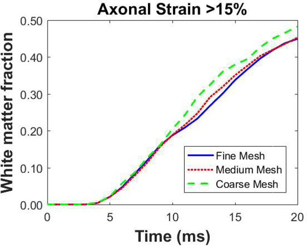
Since finite element calculations can be affected by the mesh size, we conducted a mesh sensitivity analysis. A constant angular acceleration is applied to three mesh sizes: (1) Fine mesh with max element size of 1 mm (2) Medium mesh with max element size of 2 mm (3) Coarse mesh with max element size of 4 mm. For the medium and coarse meshes, elements were a combination of four and three node plane strain elements while the fine mesh is composed of only four node plane strain elements (by converting MRI voxels directly to elements). For each mesh, we examine the evolution of the area fraction of white matter that has been deformed to axonal strains (strain along the fiber direction) greater than some threshold (Fig. 3 shows the mesh convergence results for one of the examined thresholds, which is 15%). For all strain thresholds/levels, we observe that the difference between the fine and medium meshes is smaller than the difference between medium and coarse meshes. We have also examined convergence with respect to the locations of the largest damage. Given this convergence, we selected the medium mesh for the results presented here.
FIGURE 3.
Examination of mesh convergence in the shear anisotropic model for the particular case of the axial cross-section (we expect similar results for the other cross-sections). The evolution of white matter area fraction that sustains axonal strains greater than 15% is presented as a function of time for three mesh sizes: fine (max. element size = 1 mm), medium (max. element size = 2 mm) and coarse (max element size = 4 mm). The same analysis is performed for multiple axonal strain thresholds and all revealed similar results.
Validation of the Head Model for Non-Injurious Loading
Accurate modelling of the brain tissue is a key factor in determining the level of injury during traumatic events. We validate our head model by simulating the in-vivo brain rotational motion experiment of Knutsen et al.18 Volunteers with no history of brain injury used a device that induces a non-injurious rotation about the horizontal/axial plane of the head inside the MRI at Henry Jackson Foundation (HJF). The tagged MRI technique was then used to extract the 3D brain motions. The acceleration profile obtained from the experiment is applied to the axial slice of our model, and the resulting computed shear strains are compared to the experimental values.
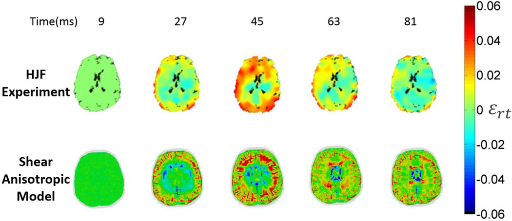
Figure 4 shows the computed shear strains in the axial slice from our shear anisotropic model (Eq. 6) and from the HJF experiment at four times. These times are based on the experimental data, which were collected and processed every 18 ms, beginning 9 ms after the loading. The evolution of shear strain is captured by the model in the following senses. After 45 ms, both the experiment and the model have the maximum shear strains reaching the middle of the brain, indicating consistent shear wave speed, and the locations of maximum and minimum strains are generally consistent between the simulation and the experiment.
FIGURE 4.
Comparison of the measured (HJF) and the computed (shear anisotropic model) shear strain distributions for the axial cross-section for every 18 ms beginning 9 ms after loading. Note that the simulation resolution is higher than the experimental resolution, leading to the appearance of more detailed strain distributions in the model results. The HJF results are derived from the18 paper.
To quantify this full field spatial validation for the model, we examine the statistical level of agreement using four different tests discussed by Ganpule et al.11: (1) index of agreement (dr) (2) coefficient of efficiency (E2) (3) root mean squared error (RMSE) to observations standard deviation Ratio (RSR) and (4) correlation score (CS) (Table 3). For these statistical measures, we define the measured shear strains from the HJF experiment as the observed data Oi, and the results from our shear anisotropic model simulation as the predicted data Pi. Table 4 shows the results of all the statistical measures. For dr;41 E220 and RSR,23 the results are closer to the “better” end of the range (the upper end for dr and E2 and the lower end for RSR). Unfortunately, these particular metrics do not yet have a defined “level of goodness”. For the CS results, the first two time frames (27 and 45 ms) are classified as fair agreement while the last two time frames (63 and 81 ms) are classified as marginal agreement.14 However, since our model is intended to be used for injurious loading which typically lasts between 15 and 36 ms, we find the overall statistical results to be acceptable.
TABLE 3.
Some measures of agreement between observations and predictions that can be used to assess TBI models.
| Level of agreement test | Formula | Range | Agreement rating |
|---|---|---|---|
| Index of agreement dr | − 1 to 1 | ↑ dr ≡ better agreement | |
| Coefficient of efficiency (E2) | − ∞ to 1 | ↑ E2 ≡ better agreement | |
| RMSE to observations | |||
| Standard deviation ratio (RSR) | 0 to ∞ | ↓ RSR ≡ better agreement | |
| Correlation score (CS) |
|
0–100 | 86–100 excellent 65–86 good 44–65 fair 26–44 marginal 0–26 unacceptable |
TABLE 4.
The degree of agreement between the shear anisotropic model and the HJF experiment at four specific times, using the measures described in Table 3.
| Time (ms) | 27 | 45 | 63 | 81 |
| dr | 0.42 | 0.23 | 0.28 | 0.29 |
| E2 | − 0.28 | − 0.98 | − 0.73 | − 0.66 |
| RSR | 1.13 | 1.40 | 1.31 | 1.29 |
| CS | 53.70 | 47.16 | 39.44 | 42.29 |
The simulation, of course, has some advantages over the experiment: higher temporal resolution and higher structural resolution. While the experimental data is available only every 18 ms, the simulation data can be extracted with much finer resolution, e.g. every millisecond. Since injurious loading usually lasts from 15 to 30 ms, the simulation produces a finer sense of the evolution of strains. Moreover, the experiment does not capture strains within the ventricles, which could affect the calculated strains in the surrounding tissues. We note also that Knutsen et al.18 eliminated rigid body rotation only at the first part of the experiment (before the head stops completely by 3–4 degrees), but did not correct for rigid body motion afterwards. Other discrepancies between the experiment and the simulation could arise from structural differences between the subject heads in the experiment and the computation, or the large spacing of the experimental tag lines in comparison with simulation element size (8 mm as compared to 1–2 mm).
Injury Criteria
Defining an injury threshold for mTBI remains very difficult. No single injury threshold has yet been globally accepted. The difficulty arises because of the contribution of so many factors in any traumatic event, including but not limited to: location of impact (if any), direction of motion, rotational and translational accelerations, duration of the event, nature of the subject’s neck, age and so forth. Accordingly multiple biomechanical thresholds have been used in the literature such as coup and contrecoup pressure,38 von Mises stress,16 principal strains,16 strain rate15 and axonal strains.42 Since our new model is intended to better describe the white matter tissue, we selected the axonal strain injury threshold. Bain and Meaney1 tested the optic nerves of guinea pigs at starin rates of 30–60 s−21 and suggested an optimal threshold for axonal strain injury of 18% (Note: the simulations in our study use strain rates of 25 s−21 based on the time of onset of damage). In our simulations (using both models), the elements are only labeled as “injured” once they reach or exceed the injury threshold of axonal strain ≥ 18%. They continue to carry load and to deform after the threshold, but once identified as injured, they remain labeled as injured throughout the simulation even if the axonal strain decreases in the next timesteps.
An Injurious Event
We now assign the known injury-causing loading conditions for each model/orientation (sagittal, coronal and axial). A reconstructed NHL incident previously used by Wright et al.42 is examined, so as to directly compare model results. For each orientation, the corresponding linear and angular accelerations are applied in explicit FE simulations. Since the known loading curves42 have a duration of only 15 ms and cutoff at non-zero values, we extend the curves so that the acceleration magnitudes are linearly decreased to zero over 5 ms (and remain zero thereafter). However, the total simulation time is determined by the time needed for shear wave propagation inside the brain.11 The simulations are stopped when the damage of white matter ceases to evolve (change in damage of 0.25% or less for three consecutive milliseconds) in all loading cases.
RESULTS
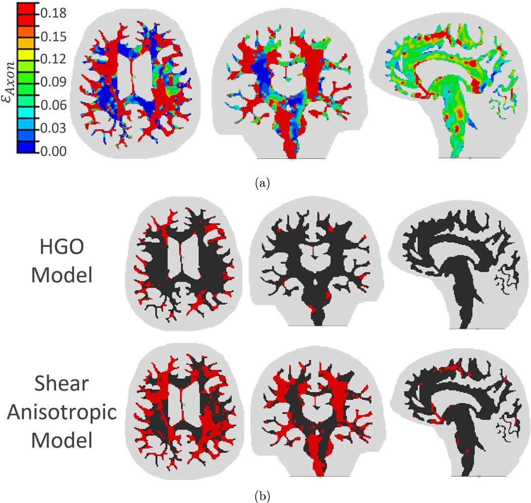
The shear anisotropy simulation results for the injury case are presented in Fig. 5a in terms of the axonal strain (damage) distributions in the three cross-sections. The degree of damage in each case is quite different from that previously obtained by Wright et al.42 using the HGO model with only tension anisotropy.
FIGURE 5.
Simulation results for: (a) The shear anisotropy of the injury case are presented in terms of the axonal strain (damage) distributions in the three cross-sections. Note: If axonal strain reached or exceeded the threshold of 18%, the element is labeled “damaged” for the remainder of the simulation. (b) The comparison of the injury predictions of the previous HGO model and the current shear anisotropic model. Damaged regions (εAxon ≥ 18%) in each slice shown in red for the axial (left), coronal (middle) and sagittal (right) orientations.
The injury levels predicted by the two models are compared in Fig. 5b. Red areas in the figure indicate elements of white matter in which the axonal strain reached or exceeded the injury threshold of 18% (any element that fulfills the injury criterion is considered damaged for the rest of the simulation). Overall, the damage predicted by the shear anisotropic model is clearly higher than the HGO model predictions.
Beside comparing damage location, the area of damage in each slice was also investigated. The percentage of damaged area Ω, is calculated as
| (10) |
where AεAxon > 18% is area of white matter elements with axonal strain exceeding 18% and AWM is the white matter area.
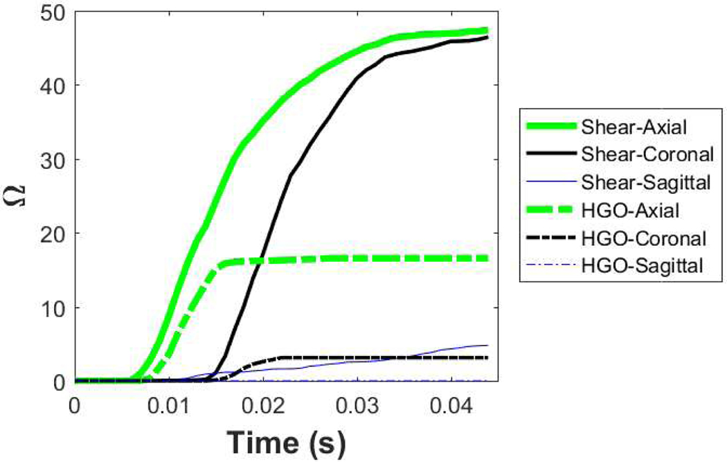
Using Eq. (10), the percent damage for each slice predicted by both models are calculated. In the axial slice, the predicted damage by the shear anisotropic model is almost three times the value predicted by the HGO model and the coronal and the sagittal slices also show more damage (compare values at end of simulations in Fig. 6).
FIGURE 6.
Time evolution of the total damage predicted by the HGO and shear anisotropic models. Solid lines represent the shear anisotropic model and dashed lines represent the HGO model. Note the higher amounts of damage predicted by the shear anisotropic model.
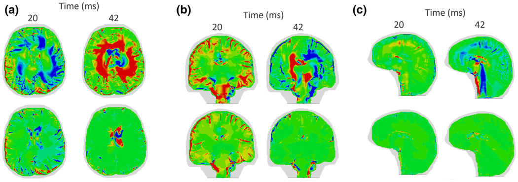
In addition to damage comparison, radial-circumferential shear strains are compared for the two models as shown in Fig. 7. For all orientations, the overall shear strains are higher in the shear anisotropic model (top row of each sub-figure) compared to the HGO shear strains (bottom row of each sub-figure). This observation is also mainly due to the difference in material properties between the shear anisotropic model and the HGO model.
FIGURE 7.
Comparisons of the evolution of the radial-circumferential shear strains predicted by the shear anisotropic model (top row) and the HGO model (bottom row) in the (a) Axial (b) Coronal and (c) Sagittal orientations. Note the shear strain concentrations in the brainstem predicted by the shear anisotropic model in the coronal and sagittal cases.
DISCUSSION
Significant differences in resultant damage between the two models are evident, as shown in Fig. 5b.We note that most computational models show damage primarily at the boundaries between white and gray matters, due to the differences in stiffness between the two tissues. However, using the shear anisotropic model, some damage begins and remains in the deep white matter tissue, away from the boundaries between white and gray matters. This observation is supported by MRI studies on both animal and human injuries21 and the work of Smith and Meaney32 in which diffuse axonal injury was characterized to be deeper in the white matter.
We find it useful to examine the damage history, i.e. the progress of damage throughout all time-frames of the simulation. Figure 6 shows the damage predicted by the shear anisotropic (solid lines) and the HGO (dashed lines) models as a function of time. The damage in the axial slice was not only higher than the other cases but also developed over a longer time. This is consistent with the loading conditions, and more specifically the angular acceleration in the z direction (applied to the axial slice) which has the maximum magnitude compared to the other two directions (applied to coronal and sagittal slices). Nevertheless, the damage predicted by the HGO model stops evolving as soon as the loading is stopped at 15 ms while in the shear anisotropic model, the damage continued increasing until around 40 ms. This may be because of the slower shear wave speed in the shear anisotropic model (0.5 m/s compared to 2.4 m/s in the HGO model).
A comparison of the radial-circumferential shear strains reveals differences between the two models in addition to the damage differences. For the coronal and the sagittal slices, the shear anisotropic model predicts higher levels of shear strains (Figs. 7b and 7c) and damage in the brainstem. Such damage is not seen in the HGO simulation. Montgomery et al.22 examined mild traumatic brain injury patients and found that the majority of the patients had abnormal brainstem function even after six weeks from the injury. Another study by Delano-Wood et al.6 on veterans with chronic mild to moderate traumatic brain injury revealed a link between brainstem white matter integrity and the loss of consciousness after the injury. Due to the inclusion of shear anisotropy in the shear anisotropic model, the brainstem experiences higher shear strains which translate to higher predicted damage compared to HGO predictions (Fig. 5b). Note, however, that our simulations include only one family of fibers in each element.
Our simulations using our validated material model strongly suggest that considering shear anisotropy (addition of I5) is important for computational predictions of mTBI. The injury predictions of the shear anisotropic model are significantly different than those predicted by the HGO model in terms of level of injury, location of injury and shear sensitivity. Although the injury threshold that we use is often used in the literature, we believe that more work is needed to correlate the symptoms presented by the injured subject with the predicted damage outcomes. Further, since the real fiber network of the brain has many crossing fibers, the shear anisotropic model needs to be improved to accommodate multiple families of fibers. Finally, we intend to extend this work for full 3D simulations of brain injury.
ACKNOWLEDGMENTS
The first author (FM) appreciates the support of Kuwait University through a scholarship. The second author (KTR) acknowledges support from the National Institute of Neurological Disorders and Strokes, National Institutes of Health (Project # R01NS055951). The authors also thank Dr. Andrew Knutsen and Dr. Dzung Pham from the Henry Jackson Foundation for sharing tagged-MRI experimental data from Knutsen et al., J Biomechanics (2014). The authors also appreciate discussions and support from Dr. Shailesh Ganpule.
Footnotes
Source: Center for Disease Control and Prevention http://www.cdc.gov/traumaticbraininjury/data/rates.html.
CONFLICT OF INTEREST
The authors have no conflict of interest to declare.
REFERENCES
- 1.Bain AC and Meaney DF Tissue-level thresholds for axonal damage in an experimental model of central nervous system white matter injury. J. Biomech. Eng. Trans. ASME 122:615–622, 2000. [DOI] [PubMed] [Google Scholar]
- 2.Begonia M, Prabhu R, Liao J, Horstemeyer M, and Williams L. The influence of strain rate dependency on the structure-property relations of porcine brain. Ann. Biomed. Eng 38:3043–3057, 2010. [DOI] [PubMed] [Google Scholar]
- 3.Chatelin S, Deck C, Renard F, Kremer S, Heinrich C, Armspach JP, and Willinger R. Computation of axonal elongation in head trauma finite element simulation. J. Mech. Behav. Biomed. Mater 4:1905–1919, 2011. [DOI] [PubMed] [Google Scholar]
- 4.Cloots R, Van Dommelen J, Nyberg T, Kleiven S, and Geers M. Micromechanics of diffuse axonal injury: influence of axonal orientation and anisotropy. Biomech. Model. Mechanobiol 10:413–422, 2011. [DOI] [PubMed] [Google Scholar]
- 5.Colgan NC, Gilchrist MD, and Curran KM Applying dti white matter orientations to finite element head models to examine diffuse tbi under high rotational accelerations. Prog. Biophys. Mol. Biol 103:304–309, 2010. [DOI] [PubMed] [Google Scholar]
- 6.Delano-Wood L, Bangen KJ, Sorg SF, Clark AL, Schiehser DM, Luc N, Bondi MW, Werhane M, Kim RT, and Bigler ED Brainstem white matter integrity is related to loss of consciousness and postconcussive symptomatology in veterans with chronic mild to moderate traumatic brain injury. Brain Imaging Behav. 9:500–512, 2015. [DOI] [PubMed] [Google Scholar]
- 7.Donnelly B. and Medige J. Shear properties of human brain tissue. J. Biomech. Eng 119:423, 1997. [DOI] [PubMed] [Google Scholar]
- 8.DVBIC. Defense and veterans brain injury center: dod worldwide numbers for tbi. http://dvbic.dcoe.mil/dod-worldwide-numbers-tbi, 2018.
- 9.El Sayed T, Mota A, Fraternali F, and Ortiz M. Biomechanics of traumatic brain injury. Comput. Methods Appl. Mech. Eng 197:4692–4701, 2008. [Google Scholar]
- 10.Estes MS and McElhaney JH Response of brain tissue of compressive loading. In: The Fourth ASME Biomechanics Conference 1970. [Google Scholar]
- 11.Ganpule S, Daphalapurkar NP, Ramesh KT, Knutsen AK, Pham DL, Bayly PV, and Prince JL A three-dimensional computational human head model that captures live human brain dynamics. J. Neurotrauma 34:2154–2166, 2017. [DOI] [PMC free article] [PubMed] [Google Scholar]
- 12.Holzapfel GA Nonlinear Solid Mechanics: A Continuum Approach for Engineering. Chichester, NY: Wiley, xiv, 2000. [Google Scholar]
- 13.Jin X, Zhu F, Mao HJ, Shen M, and Yang KH A comprehensive experimental study on material properties of human brain tissue. J. Biomech 46:2795–2801, 2013. [DOI] [PubMed] [Google Scholar]
- 14.Kimpara H, Nakahira Y, Iwamoto M, Miki K, Ichihara K, Kawano S, and Taguchi T. Investigation of anteroposterior head-neck responses during severe frontal impacts using a brain-spinal cord complex fe model. Stapp Car Crash J. 50:509–544, 2006. [DOI] [PubMed] [Google Scholar]
- 15.King AI, Yang KH, Zhang L, Hardy W, Center B, and Viano DC Is head injury caused by linear or angular acceleration? IRCOBI Conference—Lisbon (Portugal), 2003. [Google Scholar]
- 16.Kleiven S. Predictors for traumatic brain injuries evaluated through accident reconstructions. 51st Stapp Car Crash J., pp. 81–114, 2007. [DOI] [PubMed] [Google Scholar]
- 17.Kleiven S. and von Holst H. Consequences of head size following trauma to the human head. J. Biomech 35:153–160, 2002. [DOI] [PubMed] [Google Scholar]
- 18.Knutsen AK, Magrath E, McEntee JE, Xing F, Prince JL, Bayly PV, Butman JA, and Pham DL Improved measurement of brain deformation during mild head acceleration using a novel tagged mri sequence. J. Biomech 47:3475–3481, 2014. [DOI] [PMC free article] [PubMed] [Google Scholar]
- 19.Lanir Y. Constitutive-equations for fibrous connective tissues. J. Biomech 16:1–12, 1983. [DOI] [PubMed] [Google Scholar]
- 20.Legates DR and McCabe GJ Evaluating the use of “goodness-of-fit” measures in hydrologic and hydroclimatic model validation. Water Resour. Res 35:233–241, 1999. [Google Scholar]
- 21.Margulies SS and Thibault LE A proposed tolerance criterion for diffuse axonal injury in man. J. Biomech 25:917–923, 1992. [DOI] [PubMed] [Google Scholar]
- 22.Montgomery EA, Fenton GW, McClelland RJ, Macflynn G, and Rutherford WH The psychobiology of minor head-injury. Psychol. Med 21:375–384, 1991. [DOI] [PubMed] [Google Scholar]
- 23.Moriasi DN, Arnold JG, Van Liew MW, Bingner RL, Harmel RD, and Veith TL Model evaluation guidelines for systematic quantification of accuracy in watershed simulations. Trans. ASABE 50:885–900, 2007. [Google Scholar]
- 24.Nicolle S, Lounis M, and Willinger R. Shear properties of brain tissue over a frequency range relevant for automotive impact situations: new experimental results. Stapp Car Crash J. 48:239–258, 2004. [DOI] [PubMed] [Google Scholar]
- 25.Nicolle S, Lounis M, Willinger R, and Palierne JF Shear linear behavior of brain tissue over a large frequency range. Biorheology 42:209–223, 2005. [PubMed] [Google Scholar]
- 26.Ning X, Zhu Q, Lanir Y, and Margulies S. A transversely isotropic viscoelastic constitutive equation for brainstem undergoing finite deformation. J. Biomech. Eng. Trans. ASME 128:925–933, 2006. [DOI] [PubMed] [Google Scholar]
- 27.Prange MT and Margulies SS Regional, directional, and age-dependent properties of the brain undergoing large deformation. J. Biomech. Eng. Trans. ASME 124:244–252, 2002. [DOI] [PubMed] [Google Scholar]
- 28.Rashid B, Destrade M, and Gilchrist MD Mechanical characterization of brain tissue in compression at dynamic strain rates. J. Mech. Behav. Biomed. Mater. 23–38, 2012. [DOI] [PubMed] [Google Scholar]
- 29.Roberts JC, Harrigan TP, Ward EE, Taylor TM, Annett MS, and Merkle AC Human head-neck computational model for assessing blast injury. J. Biomech 45:2899–2906, 2012. [DOI] [PubMed] [Google Scholar]
- 30.Ruan JS, Khalil TB, and King AI Finite element modeling of direct head impact. Report 0148–7191, SAE Technical Paper, 1993. [Google Scholar]
- 31.Shugar TA and Katona MG Development of finiteelement head-injury model. J. Eng. Mech. Div. ASCE 101:223–239, 1975. [Google Scholar]
- 32.Smith DH and Meaney DF Axonal damage in traumatic brain injury. Neuroscientist 6:483–495, 2000. [Google Scholar]
- 33.Spencer AJM Deformations of Fibre-Reinforced Materials. Oxford: Clarendon Press, 1972. [Google Scholar]
- 34.Takhounts E, Eppinger R, Campbell J, Tannous R, Power E, and Shook L. On the development of the simon finite element head model. Stapp Car Crash J. 47:107–133, 2003. [DOI] [PubMed] [Google Scholar]
- 35.Tamura A, Hayashi S, Nagayama K, and Matsumoto T. Mechanical characterization of brain tissue in high-rate extension. J. Biomech. Sci. Eng 3:263–274, 2008. [Google Scholar]
- 36.Taylor PA and Ford CC Simulation of blast-induced early-time intracranial wave physics leading to traumatic brain injury. J. Biomech. Eng. Trans. ASME 131, 2009. [DOI] [PubMed] [Google Scholar]
- 37.Velardi F, Fraternali F, and Angelillo M. Anisotropic constitutive equations and experimental tensile behavior of brain tissue. Biomech. Model. Mechanobiol 5:53–61, 2006. [DOI] [PubMed] [Google Scholar]
- 38.Ward C, Chang M, and Nahum A. Intracranial pressure—a brain injury criterion. In: 26th Stapp Car Crash Conference Proceedings SAE 801304, 1980. [Google Scholar]
- 39.Ward CC and Thompson RB The development of a detailed finite element brain model. In: Report 0148–7191, SAE Technical Paper, 1975. [Google Scholar]
- 40.Watanabe D, Yuge K, Nishimoto T, Murakami S, and Takao H. Development of a human head fe model and impact simulation on the focal brain injury. J. Comput. Sci. Technol 3:252–263, 2009. [Google Scholar]
- 41.Willmott CJ, Robeson SM, and Matsuura K. A refined index of model performance. Int. J. Climatol 32:2088–2094, 2012. [Google Scholar]
- 42.Wright RM, Post A, Hoshizaki B, and Ramesh KT A multiscale computational approach to estimating axonal damage under inertial loading of the head. J. Neurotrauma 30:102–118, 2013. [DOI] [PubMed] [Google Scholar]
- 43.Wright RM and Ramesh KT An axonal strain injury criterion for traumatic brain injury. Biomech. Model. Mechanobiol 11:245–260, 2012. [DOI] [PubMed] [Google Scholar]
- 44.Yao JF, Yang JK, and Otte D. Investigation of head injuries by reconstructions of real-world vehicle-versusadult-pedestrian accidents. Saf. Sci 46:1103–1114, 2008. [Google Scholar]
- 45.Zhang LY, Yang KH, and King AI Comparison of brain responses between frontal and lateral impacts by finite element modeling. J. Neurotrauma 18:21–30, 2001. [DOI] [PubMed] [Google Scholar]
- 46.Zhang LY, Yang KH, and King AI A proposed injury threshold for introduction mild traumatic brain injury. J. Biomech. Eng. Trans. ASME 126:226–236, 2004. [DOI] [PubMed] [Google Scholar]
- 47.Zhou C, Khalil T, and King AI Shear stress distribution in the porcine brain due to rotational impact. In: 38th Stapp Car Crash Conference Proceedings SAE 942314, 1994. [Google Scholar]


