Abstract
As of July 2020, COVID-19 caused by SARS-COV-2 is spreading worldwide, causing severe economic damage. While minimizing human contact is effective in managing outbreaks, it causes severe economic losses. Strategies to solve this dilemma by considering the interrelation between the spread of the virus and economic activities are urgently needed to mitigate the health and economic damage. Here, we propose an abstract agent-based model of the COVID-19 outbreak that accounts for economic activities. The computational simulation of the model recapitulates the trade-off between the health and economic damage associated with voluntary restraint measures. Based on the simulation results, we discuss how the macroscopic dynamics of infection and economics emerge from individuals’ behaviours. We believe our model can serve as a platform for discussing solutions to the above-mentioned dilemma.
Keywords: COVID-19, economy, infection, agent-based model
1. Introduction
COVID-19, caused by SARS-COV-2, was first reported in Wuhan in December 2019 [1–6]; it spread globally, causing severe health and economic damage. By 29 July 2020, over 16 million people had tested positive and 660 thousand people had died due to COVID-19 [7]. From the economic perspective, many people suffered losses and lost their jobs [8]. Therefore, we find a dilemma between mitigating the spread of COVID-19 and reducing economic losses, that is, strategies to decrease contact between humans, such as voluntary restraint and social distancing, hinder normal economic activities. Hence, solving this dilemma by finding strategies to mitigate the outbreak while minimizing economic losses is an urgent issue.
Many mathematical models of the spread of infectious diseases have been proposed using differential equations [9–12] and agent-based models [13–15], and several studies focus on the spread of COVID-19 in various contexts [16–26]. These studies model only the spread of infectious diseases and do not describe economic activities mathematically. Other studies focused on the economic impacts of COVID-19 [27–31], some of which considered economic processes in detail and predicted economic impacts under realistic assumptions [27–29]; thus, they are complex and make it difficult to capture the essence of the interrelation between the spread of the virus and economic activities. Other studies estimated the economic impact using a simple model based on differential equations [30,31]. While these models describe the economic effects at the population level, the effects of individuals’ behaviours on the macroscopic dynamics of infection and the economy remain unclear. A definitive mathematical model that captures the essential mechanism of the interrelation between the spread of the virus and economic activities at an individual level could fill this gap.
In this study, we propose a simple mathematical model that considers both COVID-19 infections and economic activities. Our aim is to extract the essence of the relationship between the spread of COVID-19 and economic activities, rather than making a quantitative and accurate prediction of infection and economic outcomes. Moreover, we are interested in how the macroscopic dynamics of infection and economic effects emerge from individuals’ behaviours, rather than a coarse macroscopic description. Hence, we propose a highly abstract and simple agent-based model without employing detailed and realistic assumptions. More specifically, we propose a cellular automaton model in which mobile agents with internal states regarding infection and the economy interact with others and update their internal states. Through simulations, we demonstrate how the health and economic states evolve depending on several parameters. Based on the results, we discuss the effect of voluntary restraint.
2. Model
(a). Overview of the proposed model
We consider a cellular automaton model in which hexagonal cells are aligned regularly on a two-dimensional plane (figure 1) with N agents. Each agent has a home cell and can stay at home or move to its adjacent cell at each time step. Each agent has a health state Statei and money Mi, which are updated through interaction with other agents. Agents die when they do not recover after infection or when their money becomes zero.
Figure 1.
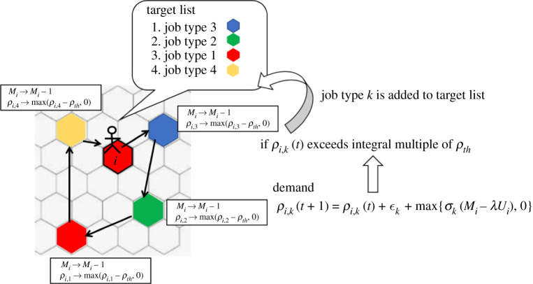
Outline of the proposed model. When ρi,k(t) exceeds the integral multiple of ρth, job type k is added to the bottom of the target list of agent i. Agent i visits the home of the nearest agent among the agents whose job type corresponds to the top of the target list. When the agent reaches the home, the agent pays a unit amount of money to buy goods. Then because the demand of agent i is satisfied, ρi,k decreases by ρth. The top item in the target list is removed, and the other items in the target list move up. Then, agent i visits the next target. When there are no items in the target list, agent i returns home and remains there. (Online version in colour.)
Agents have their own businesses. There are several types of businesses that range from selling commodities to selling non-essentials. Each agent chooses one type among them and does not change temporarily. Each agent has a demand for goods. When the demand exceeds a certain threshold, the agent goes out to buy them. The agent pays money when it reaches the home of an agent who sells the goods (figure 1). We assume that agent i sells goods to agent j when agent j visits the home cell of agent i. The model does not include the prime costs of goods. When agents perceive that infection is spreading around themselves, they tend not to demand non-essentials, while they demand commodities as usual. In the following subsections, we describe the details of the proposed model.
(b). Model of infection
We model the spread of COVID-19 by drawing inspiration from a spatial susceptible-exposed-infectious-recovered (SEIR) model [15]. Each agent has a health state Statei, which has a susceptibility state (S), an asymptomatic infection state (E), a symptomatic infection state (I), a quarantine state (Q), a recovered state (R) and a death state (D).
The state changes according to the rule in figure 2. When an agent with state S is in a cell occupied by an agent with state E or I, Statei changes from S to E with probability pE at every time step. Here, although the existing SEIR model [15] assumes that only agents with state I have infectability, we assume that agents with states E or I have infectability because asymptomatic COVID-19 patients have infectability [32]. When τE time steps pass after the transition from state S to E, the state changes to state I. Agents with state I change to state Q and D with probability pD and pQ, respectively, at every time step. Agents with state Q, which represents hospitalized patients, do not have infectability and stop any economic activity described in the next subsection. Agents with state Q also die with probability pD at every time step. Regardless of whether quarantined or not, the state changes to R when τR time steps pass after the transition from state E to I.
Figure 2.
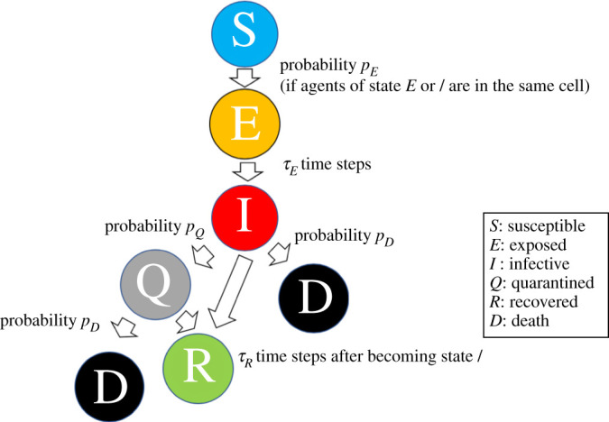
Rule for the transition of the health state. (Online version in colour.)
(c). Model of economic activity
Each agent has money Mi, which increases and decreases when other agents buy agent i’s goods and when agent i buys goods, respectively. We assume that the price of all goods is one unit, which does not change temporarily. Namely, when agent i sells a good to agent j, Mi and Mj increase and decrease by one, respectively. In addition to buying and selling, high-income people pay high taxes, while low-income people receive public assistance in real societies. Although these policies are complex, we simply assume that the money of each agent increases and decreases with these policies when their economic levels are below and above the average level, respectively. Thus, we describe the time evolution of Mi as
| 2.1 |
where t is a time step, K and are positive constants and qin,i(t) and qout,i(t) denote the amount of money that increases or decreases via selling and buying, respectively. The fourth term on the right-hand side represents the effect of income redistribution: high-income people pay high taxes and low-income people receive public assistance. The parameter K represents the extent of the income redistribution policy. Agent i dies when Mi(t) becomes zero.
Each agent chooses from one of m job types, which does not change temporarily. Agent i’s demand for goods produced by job types k (i = 1, 2, …, N and k = 1, 2, …, m) are denoted by ρi,k. The time evolution of ρi,k is
| 2.2 |
where ϵk, σk and λ are positive constants, and Ui quantifies agent i’s perception of ‘the extent to which infection is spreading around itself’, which we formulate below. Parameter ϵk represents the rate of increase in the demand which does not depend on the money agent i owns or the degree of the outbreak. By contrast, σk represents the rate of increase in demand which is affected by the money agent i owns or the degree of the outbreak. The third term on the right-hand side of equation (2.2) means that the demand increases rapidly when agent i has a lot of money, though the increase stops under the outbreak. Parameter λ represents the degree of voluntary restraint under an outbreak. We set ϵk and σk to be large and small, respectively, when job type k is related to commodities, and vice versa when job type k is related to non-essentials. Namely, demand for commodities increases constantly regardless of the economic state and the state of outbreak, while those for non-essentials are affected by the amount of money agents own and the degree of outbreak.
Agent i’s perception of the spread of infection Ui is
| 2.3 |
where ni is the number of agents with state Q within radius r from agent i, which represents the number of patients monitored in the residential area. Here, we count only the number of quarantined agents based on the assumption that people cannot recognize that people with states E and I are actually infected. Equation (2.3) means that Ui(t) increases or decreases, followed by an increase or decrease in ni(t). Ui(t) is updated rapidly when κ is large. Thus, κ characterizes the delay between the actual and perceived disease spread (increase in hospitalized patients) around agent i; κ increases as the delay decreases.
Each agent has a target list that represents the priority of goods to purchase (figure 1). When the demand ρi,k exceeds the integral multiple of ρth, job type k is added to the bottom of agent i’s target list. Agent i visits the home of the nearest agent, whose job type corresponds to the top of the target list. When the agent reaches its home, it pays a unit amount of money to buy the goods. Here, we simply assume that this deal holds even when the selling agent is not at home. Then because the demand of agent i is satisfied, ρi,k decreases by ρth. The top item in the target list is removed, and the other items in the target list move up. Then, agent i visits the next target. When no items remain in the target list, agent i returns to its home cell and remains there. Here, we assume that the order in the target list is never reversed for simplicity, although people often prioritize buying commodities when they are urgently needed.
We describe the rule for the movement of each agent as follows (figure 3). First, we define the target position of agent i as the home of the nearest agent whose job type corresponds to the top of the target list. When no items remain in the target list, the target position is agent i’s home cell. We denote a unit vector that points the target position from the current position of agent i by Di. When the target position is identical to the current position, Di = 0. Agent i moves to its adjacent cells or stays in the current position with the probability pi(l):
| 2.4 |
in the case of Di ≠ 0, and
| 2.5 |
in the case of Di = 0, where figure 3 provides the definitions of the unit vector el and the subscript l. The term el · Di is positive when cell l is located near the direction of the target position and negative vice versa. Thus, owing to this term, agent i tends to approach the target position.
Figure 3.
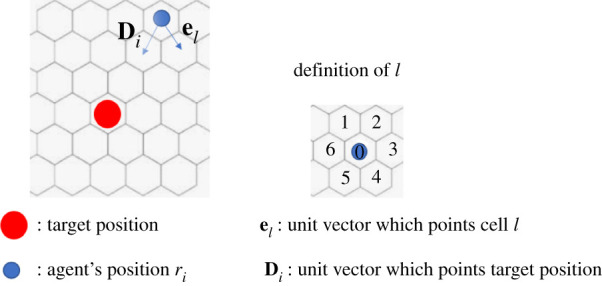
Definition of Di and el. (Online version in colour.)
3. Simulation results
We performed simulations of the proposed model. The number of cells along the horizontal and vertical directions are 43 and 50, respectively, and we adopt the periodic boundary condition. Except for the experiment illustrated in figure 4, we set the total number of agents N to 1000. We set the initial amount of money to for all agents. We placed the home cells of the agents randomly without any overlap. Each agent is initially located at its home. We performed each trial for 30 000 time steps.
Figure 4.
Simulation results when N and λ change. (a) and (b) show Dinf/N and Deco/N, respectively. (Online version in colour.)
The simulation contains four job types, with an identical number of people for each job type. We determine the parameters ϵk and σk (k = 1, 2, 3, 4) as
| 3.1 |
Thus, people with a high job type number sell commodities while those with a small job type number sell non-essentials. From equations (2.2) and (3.1), the rate of increase in demand ρi,k does not depend on the job type when .
We used non-dimensional parameters in the simulation. Because the proposed model is highly abstract, it is difficult to determine the parameters based on realistic data. However, we chose the duration of the latent period τE and that of infection τR to roughly mimic the properties of COVID-19. Specifically, we set τE and τR to 600 and 1200, respectively. These non-dimensional values correspond to 7 and 14 days, respectively, if each time step is rescaled to 16.8 min, and these values roughly agree with the property of COVID-19. We set the death probability pD such that the death rate becomes approximately 10% without voluntary restraint; that is, λ = 0. We determined the economic parameters such as and K such that death caused by the economic loss becomes almost zero in the absence of an outbreak, but some people die due to economic loss under voluntary restraint during an outbreak. Table 1 summarizes the parameter values, which we use unless otherwise specified hereafter.
Table 1.
Simulation parameter values.
| parameter | value | parameter | value |
|---|---|---|---|
| N | 1000 | R | 10 |
| pE | 0.012 | pD | 0.0001 |
| pQ | 0.005 | κ | 0.0004 |
| τE | 600 | τR | 1200 |
| ρth | 100.0 | K | 0.0007 |
| 60 | 60 |
(a). Results when no patient exists
To capture the basic property of the proposed model, we performed the simulations in the no patient case; that is, Statei = S holds for all i. By removing the factor of infection from the model, we can easily understand the basic property of economic activity. In this experiment, we changed the parameter K to investigate the effect of income redistribution by taxes and public assistance. We evaluate the results in terms of the number of deaths caused by economic loss Deco and the variance of the amount of money , where is the average Mi.
Supplementary videos 1–3 show the results when K = 0, 0.00007 and 0.00014, respectively. Figure 5 shows the time evolution of V[M] and Deco for several values of K. We find that V[M] increases over time. The rate of increase decreases as the value of K increases (figure 5a). The number of deaths Deco increases over time for a small K, while it remains zero for a large K (figure 5b). This result is reasonable because frequent buying and selling events cause random walk-like behaviour in Mi and make the distribution of Mi spread in a diffusive manner. The fourth term on the right-hand side of equation (2.1) suppresses the spread of the distribution of Mi. Thus, as K increases, the difference between the rich and the poor decreases, and the number of deaths caused by economic loss decreases.
Figure 5.
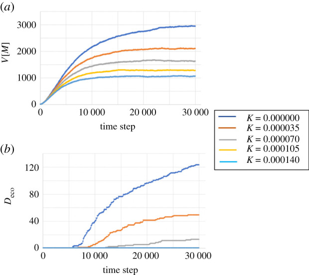
Results when no patient exists. The figure shows the time evolutions of (a) V[M] and (b) Deco for several values of K. In (b), the lines for K = 0.000105 and 0.000140 overlap. (Online version in colour.)
(b). Effects of voluntary restraint
We performed simulations for the case in which the health state changes from S to E with the probability of 0.005 at time step 5000. We set parameter K to 0.00007. We also simulated cases of λ = 0, 120 and 210 to investigate the effect of voluntary restraint.
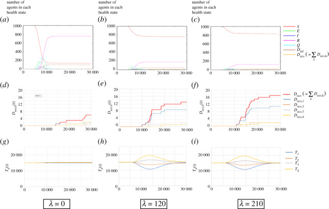
Supplementary videos 4–6 show the results when λ = 0, 120 and 210, respectively. Figures 6a–c show the time evolution of the number of agents with each health state. When λ = 0, the infection spreads rapidly and more than 80% of agents are infected. The maximum number of quarantined patients (state Q) is 278, and the number of deaths caused by infection Dinf(t) finally reached 101 (figure 6a). As λ increases, the number of patients and the deaths caused by infection decrease considerably (figures 6b,c). When λ = 210, less than 20% of the agents were infected (figure 6c).
Figure 6.
Simulation results when patients appear at time step 5000: (a)–(c) Time evolution of the number of agents in each health state (S, E, I, R, Q, Dinf and Deco); (d)–(g) time evolution of Deco,k(t) and ; and (h)–(i) time evolution of Tk(t). λ = 0 for (a), (d) and (g); 120 for (b), (e) and (h); and 210 for (c), (f ) and (i). (Online version in colour.)
Next, we observe the economic tendencies in these cases. We evaluate the results by the total number of deaths caused by economic loss and the total amount of money for each job type, denoted by Deco,k(t) and Tk(t), respectively (k = 1, 2, 3, 4). Namely, Tk(t) is given by
| 3.2 |
Figures 6d–f and g–h, respectively, illustrate the time evolution of Deco, k(t) and Tk(t) for the cases of λ = 0, 120 and 210. For λ = 0, only a few agents died because of economic loss (figure 6d). The total amount of money Tk(t) remains almost constant (figure 6g). Voluntary restraint, that is, λ > 0, generates an economic gap between job types. Specifically, Tk(t) becomes small for small k and vice versa for large k followed by the outbreak. The economic gap is the highest around 15 000 time steps, and it is mitigated gradually until around 30 000 time steps (figures 6h,i). The number of deaths caused by economic loss is larger for small k (figure 6e), and it increases as λ increases (figure 6f ). This result suggests that voluntary restraint causes agents who sell non-essentials to suffer an economic loss, while those who sell commodities do not. However, the agents suffering from an economic loss can return to their normal lives after the outbreak is over.
In summary, voluntary restraint is effective for mitigating an outbreak, although it induces an economic gap and increases the number of deaths caused by economic loss.
(c). Effect of other parameters
To further clarify the properties of the proposed model, we performed simulations by changing several parameters expected to affect the resultant behaviours. Specifically, we changed the infectious rate pE, the duration of infection τE and τR, the amount of money and , the total number of agents N, and the speed of the response to the outbreak κ, since we expect that these parameters would affect the infection and economic dynamics. For each parameter, we also changed λ and made colour maps for ease of analysis. The other simulation conditions were the same as those described in the previous subsection. We evaluate the results by the ratio of the number of deaths caused by infection Dinf to the number of agents N and that of the number of deaths caused by economic loss Deco to the number of agents N at the 30 000th time step. We performed 10 trials for each parameter and report the average values of Dinf/N and Deco/N hereafter. In the following subsections, we report the results when the parameters vary.
(i). (pE dependence)
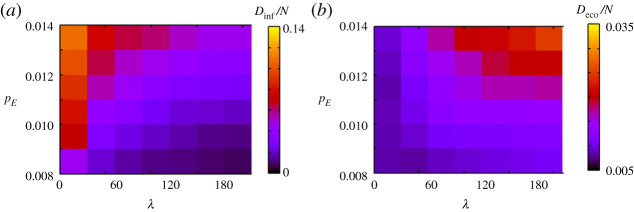
Figure 7 shows the result when we change the infectious rate pE. For small pE, Dinf/N decreases as λ increases, while Deco/N is almost unchanged depending on λ. Meanwhile, when pE is large, Dinf/N is large for small λ, while Deco/N is large for large λ. This trade-off increases in severity as the infectious rate increases. This result suggests that when the infectious rate is low, voluntary restraint can stop the outbreak before economic loss becomes severe. When the infectious rate is high, infection spreads in the absence of voluntary restraint, and even strong voluntary restraint cannot completely stop the outbreak; thus, economic loss becomes severe under strong voluntary restraint.
Figure 7.
Simulation results when pE and λ change. (a) and (b) show Dinf/N and Deco/N, respectively. (Online version in colour.)
(ii). (τE and τR dependence)
Figure 8 shows the result when we change the duration of infection τE and τR while maintaining the relation τR = 2τE. When τE and τR are small, Dinf/N decreases as λ increases, while Deco/N does not depend much on λ. When τE and τR are large, Dinf/N is large for small λ, while Deco/N is large for large λ. Thus, the above-mentioned trade-off increases in severity as the duration of infection increases. This result suggests that the increase in τE and τR has an effect similar to the increase in pE. When the duration of infection is short, voluntary restraint enables the cessation of the outbreak before economic loss becomes severe. However, it is not possible as the duration increases.
Figure 8.
Simulation results when changing τE, τR and λ while satisfying τR = 2τE. (a) and (b) show Dinf/N and Deco/N, respectively. (Online version in colour.)
(iii). ( and dependence)
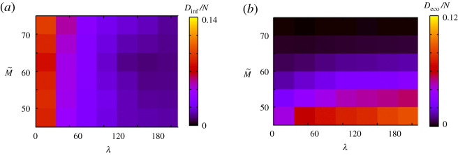
Figure 9 shows the result when we change the initial amount of money . We also change in equation (2.1) such that holds. While Dinf/N decreases as λ increases, it does not depend much on . In contrast, Deco/N increases as decreases. Thus, when people have enough money, they can continue voluntary restraint until the outbreak ends. However, when people do not have enough money, voluntary restraint leads to an increase in death caused by economic loss. Consequently, people cannot undergo severe voluntary restraint, which leads to an increase in the death caused by infection.
Figure 9.
Simulation results when and λ change. (a) and (b) show Dinf/N and Deco/N, respectively. (Online version in colour.)
(iv). (N dependence)
Figure 4 shows the result when we change the total number of agents N. When N is large, Dinf/N is large for a small λ and Deco/N is large for a large λ. This is reasonable because when N is large, people have many opportunities to meet others, and thus the probability of infection is high. When people adopt voluntary restraint, the death caused by economic loss increases. When N is small, Dinf/N is generally small, and Deco/N is not significantly affected by λ. In this case, few people are infected because they have few opportunities to meet others. The reason some people die due to economic loss is not related to infection. As figure 5b (K = 0.00007) shows, a few people die due to economic loss even in the absence of infection.
(v). (κ dependence)
Figure 10 shows the result when we vary the speed of the response to the outbreak κ. When κ is small, Dinf/N tends to be larger than in the case of large κ, and Deco/N is large for a large λ. Meanwhile, when κ is large, Deco/N decreases as λ increases. This result suggests that the outbreak cannot be mitigated under a slow response against the spread of the virus. Under a fast response, voluntary restraint is effective because it can stop the outbreak before economic loss becomes severe. Thus, responding quickly is important for both mitigating outbreaks and maintaining economic activity.
Figure 10.
Simulation results when κ and λ change. (a) and (b) show Dinf/N and Deco/N, respectively. (Online version in colour.)
4. Discussion and conclusion
In this paper, we proposed a simple and abstract mathematical model of a COVID-19 outbreak with economic activities. The simulation results show that voluntary restraint measures can help mitigate an outbreak, although it generates an economic gap between job types. We can explain the resulting economic gap as follows: the income of agents who sell non-essentials decreases during an outbreak because demand for non-essentials decreases owing to voluntary restraint. Since they must buy commodities as usual, they become poorer. By contrast, agents who sell commodities can get income as usual, yet they do not buy non-essentials due to voluntary restraint. Consequently, they become richer. This result suggests that in real societies, governments should make efforts to reduce the economic gap; otherwise, voluntary restraint measures cannot continue, which makes it difficult to mitigate an outbreak.
From figures 4 and 7–10, whether it is possible to mitigate outbreaks while minimizing economic loss depends on various factors such as the properties of the virus, people’s economic levels and the speed of people’s responses. The result in figure 9 suggests that people cannot tolerate voluntary restraint if their overall economic level is low. Thus, it is particularly difficult for communities with low economic power to mitigate outbreaks while maintaining economic activities. A possible solution to this problem is to respond to the spread of the virus as early as possible. As figure 10 suggests, if the response occurs earlier (which corresponds to a large κ in our model), it is possible to stop an outbreak without causing severe economic damage. If people fail to respond quickly and the virus spreads, then people should anticipate other possibilities, such as the development of antiviral drugs and a weakening of the virus, which corresponds to decreasing pE in our model.
Because we did not consider production activities and simply assumed that the prime costs of goods are zero, our model is not suitable for making precise and quantitative predictions, especially on the economic impact. However, our model captures the essence of the interrelation between the spread of SARS-COV-2 and economic activities. Thus, we believe that our model can become a platform for discussing strategies to mitigate the outbreak while maintaining economic activities. Indeed, our model has many potential extensions. For example, it may be possible to account for the effect of long-distance movement with transportation modes such as airplanes and trains. Defining the capacity of hospitals may help policymakers discuss how to avoid overwhelming hospitals. It may also be interesting to introduce the individual characteristics of each agent and discuss how selfish people affect the spread of the virus and economic activities.
Moreover, beyond the outbreak of COVID-19, our model may share a common mechanism with other systems that can survive under harsh circumstances with limited resources, such as bacterial biofilms [33] and communities of vampire bats [34]. Extracting the common mechanism may lead to the establishment of a general design principle for artificial systems with high survivability.
Supplementary Material
Supplementary Material
Supplementary Material
Supplementary Material
Supplementary Material
Supplementary Material
Supplementary Material
Supplementary Material
Supplementary Material
Acknowledgements
The authors would like to thank Dr Akira Fukuhara and Shura Suzuki of the Research Institute of Electrical Communication, Tohoku University for their helpful suggestions. The authors would like to thank Dr Masahiro Shimizu of Osaka University for providing part of the source code.
Data accessibility
The data including the source code and the supplementary videos are provided as electronic supplementary material.
Authors' contributions
T.K. and M.A. conceived of the work. T.K. and K.Y. proposed the mathematical model, and T.M., M.A. and A.I. refined it. T.K. performed the simulations. All authors analysed the results and drafted the manuscript. All authors gave final approval for publication and agree to be held accountable for the work performed therein.
Competing interests
We declare we have no competing interests.
Funding
This work is in part supported by the JSPS KAKENHI Fund for the Promotion of Joint International Research (Fostering Joint International Research (B))19KK0103.
References
- 1.Li Q et al. 2020. Early transmission dynamics in Wuhan, China, of novel coronavirus-infected pneumonia. N. Engl. J. Med. 382, 1199–1207. ( 10.1056/NEJMoa2001316) [DOI] [PMC free article] [PubMed] [Google Scholar]
- 2.Zhu N et al. 2020. A novel coronavirus from patients with pneumonia in China, 2019. N. Engl. J. Med. 382, 727–733. ( 10.1056/NEJMoa2001017) [DOI] [PMC free article] [PubMed] [Google Scholar]
- 3.Rodriguez-Morales AJ et al. 2020. Clinical, laboratory and imaging features of COVID-19: a systematic review and meta-analysis. Travel. Med. Infect. Dis. 34, 101623 ( 10.1016/j.tmaid.2020.101623) [DOI] [PMC free article] [PubMed] [Google Scholar]
- 4.Nishiura H et al. 2020. The extent of transmission of novel coronavirus in Wuhan, China, 2020. J. Clin. Med. 9, 330 ( 10.3390/jcm9020330) [DOI] [PMC free article] [PubMed] [Google Scholar]
- 5.Hâncean M, Perc M, Lerner J. 2020. Early spread of COVID-19 in Romania: imported cases from Italy and human-to-human transmission networks. Roy. Soc. Open Sci. 7, 200780 ( 10.1098/rsos.200780) [DOI] [PMC free article] [PubMed] [Google Scholar]
- 6.Momtazmanesh S et al. 2020. All together to fight COVID-19. Am. J. Trop. Med. Hyg. 102, 1181–1183. ( 10.4269/ajtmh.20-0281) [DOI] [PMC free article] [PubMed] [Google Scholar]
- 7.Johns Hopkins University, Coronavirus Resource Center. https://coronavirus.jhu.edu/map.html.
- 8.Coibion O, Gorodnichenko Y, Weber M 2020 doi: 10.3386/w27017. Labor markets during the COVID-19 crisis: a preliminary view. NBER Working paper 27017. ( ) [DOI]
- 9.Kermack WO, McKendrick AG. 1927. Contributions to the mathematical theory of epidemics. Proc. R. Soc. A 115, 700–721. ( 10.1098/rspa.1927.0118) [DOI] [PubMed] [Google Scholar]
- 10.Klepac P, Pomeroy LW, Bjørnstad ON, Kuiken T, Osterhaus AD, Rijks JM. 2009. Stage-structured transmission of phocine distemper virus in the Dutch 2002 outbreak. Proc. Biol. Sci. 276, 2469–2476. ( 10.1098/rspb.2009.0175) [DOI] [PMC free article] [PubMed] [Google Scholar]
- 11.Klepac P, Caswell H. 2011. The stage-structured epidemic: linking disease and demography with a multi-state matrix approach model. Theor. Ecol. 4, 301–319. ( 10.1007/s12080-010-0079-8) [DOI] [Google Scholar]
- 12.Chowell G, Nishiura H, Bettencourt LMA. 2007. Comparative estimation of the reproduction number for pandemic influenza from daily case notification data. J. R. Soc. Interface 4, 155–166. ( 10.1098/rsif.2006.0161) [DOI] [PMC free article] [PubMed] [Google Scholar]
- 13.Carley KM, Fridsma DB, Casman E, Yahja A, Altman N, Chen LC, Kaminsky B, Nave D. 2006. BioWar: scalable agent-based model of bioattacks. IEEE Trans. Sys. Man Cybern. A 36, 252–265. ( 10.1109/TSMCA.2005.851291) [DOI] [Google Scholar]
- 14.Frias-Martinez E, Williamson G, Frias-Martinez V. 2011. An agent-based model of epidemic spread using human mobility and social network information. IEEE 3rd Int. Conf. Privacy, Security, Risk and Trust and IEEE 3rd Int. Conf. Social Computing, pp. 57–64 ( 10.1109/PASSAT/SocialCom.2011.142). [DOI]
- 15.Urabe CT, Tanaka G, Aihara K, Mimura M. 2016. Parameter scaling for epidemic size in a spatial epidemic model with mobile individuals. PLoS ONE 11, e0168127 ( 10.1371/journal.pone.0168127) [DOI] [PMC free article] [PubMed] [Google Scholar]
- 16.Currie CS, Fowler JW, Kotiadis K, Monks T, Onggo BS, Robertson DA, Tako AA. 2020. How simulation modelling can help reduce the impact of COVID-19. J. Simulation 14, 83–97. ( 10.1080/17477778.2020.1751570) [DOI] [Google Scholar]
- 17.Lin Q et al. 2020. A conceptual model for the coronavirus disease 2019 (COVID-19) outbreak in Wuhan, China with individual reaction and governmental action. Int. J. Infec. Dis. 93, 211–216. ( 10.1016/j.ijid.2020.02.058) [DOI] [PMC free article] [PubMed] [Google Scholar]
- 18.Fang Y, Nie Y, Penny M. 2020. Transmission dynamics of the COVID-19 outbreak and effectiveness of government interventions: a data-driven analysis. J. Med. Virol. 92, 645–659. ( 10.1002/jmv.25750) [DOI] [PMC free article] [PubMed] [Google Scholar]
- 19.Tang B, Wang X, Li Q, Bragazzi NL, Tang S, Xiao Y, Wu J. 2020. Estimation of the transmission risk of the 2019-nCoV and its implication for public health interventions. J. Clin. Med. 9, 462 ( 10.3390/jcm9020462) [DOI] [PMC free article] [PubMed] [Google Scholar]
- 20.Hellewell J et al. 2020. Feasibility of controlling COVID-19 outbreaks by isolation of cases and contacts. Lancet Global Health 8, 488–496. ( 10.1016/S2214-109X(20)30074-7) [DOI] [PMC free article] [PubMed] [Google Scholar]
- 21.Wells CR et al. 2020. Impact of international travel and border control measures on the global spread of the novel 2019 coronavirus outbreak. Proc. Natl Acad. Sci. USA 117, 7504–7509. ( 10.1073/pnas.2002616117) [DOI] [PMC free article] [PubMed] [Google Scholar]
- 22.Prem K et al. 2020. The effect of control strategies to reduce social mixing on outcomes of the COVID-19 epidemic in Wuhan, China: a modelling study. Lancet Public Health 5, E261–E270. ( 10.1016/S2468-2667(20)30073-6) [DOI] [PMC free article] [PubMed] [Google Scholar]
- 23.Ferguson NM et al. 2020. Impact of non-pharmaceutical interventions (NPIs) to reduce COVID-19 mortality and healthcare demand. Imperial College Covid-19 Response Team 2, 60–66 ( 10.25561/77482). [DOI]
- 24.Stutt ROH, Retkute R, Bradley M, Gilligan CA, Colvin J. 2020. A modelling framework to assess the likely effectiveness of facemasks in combination with ‘lock-down’ in managing the COVID-19 pandemic. Proc. R. Soc. A 476, 20200376 ( 10.1098/rspa.2020.0376) [DOI] [PMC free article] [PubMed] [Google Scholar]
- 25.Karin O et al. 2020. Cyclic exit strategies to suppress COVID-19 and allow economic activity. MedRxiv. ( 10.1101/2020.04.04.20053579) [DOI] [Google Scholar]
- 26.Perc M, Miksić NG, Slavinec M, Stožer A. 2020. Forecasting COVID-19. Front. Phys. 8, 127 ( 10.3389/fphy.2020.00127) [DOI] [Google Scholar]
- 27.Favero C, Ichino A, Rustichini A. 2020. Restarting the economy while saving lives under Covid-19. CEPR Discussion paper No. DP14664 ( 10.2139/ssrn.3580626). [DOI]
- 28.Brotherhood L, Santos C, Kircher P, Tertilt M. 2020. An economic model of the COVID-19 epidemic: the importance of testing and age-specific policies. IZA DP No. 13265.
- 29.McKibbin WJ, Fernando R. 2020. The global macroeconomic impacts of COVID-19. CAMA Working paper 19.
- 30.Atkeson A 2020. What will be the economic impact of COVID-19 in the US? Rough estimates of disease scenarios. NBER Working Paper 26867.
- 31.Toda AA 2020. Susceptible-Infected-Recovered (SIR) dynamics of COVID-19 and economic impact. (http://arxiv.org/abs/2003.11221).
- 32.Huang L, Zhang X, Zhang X, Wei Z, Zhang L, Xu J, Liang P, Xu Y, Zhang C, Xu A. 2020. Rapid asymptomatic transmission of COVID-19 during the incubation period demonstrating strong infectivity in a cluster of youngsters aged 16-23 years outside Wuhan and characteristics of young patients with COVID-19: A prospective contact-tracing study. J. Infection 80, e1–e13. ( 10.1016/j.jinf.2020.03.006) [DOI] [PMC free article] [PubMed] [Google Scholar]
- 33.Mikami T, Asally M, Kano T, Ishiguro A. 2019. A reaction–diffusion model for simulating the oscillatory expansion of biofilms. Conf. Artificial Life (ALIFE), pp. 218–219 ( 10.1162/isal_a_00164). [DOI]
- 34.Mikami T, Kano T, Ishiguro A. 2020. An agent-based model for community formation process of vampire bats that survive by sharing food. J. Artifi. Life Rob. 25, 561–568. ( 10.1007/s10015-020-00649-9) [DOI] [Google Scholar]
Associated Data
This section collects any data citations, data availability statements, or supplementary materials included in this article.
Supplementary Materials
Data Availability Statement
The data including the source code and the supplementary videos are provided as electronic supplementary material.


