Face mask detection using YOLOv3 and faster R-CNN models: COVID-19 environment

Abstract

There are many solutions to prevent the spread of the COVID-19 virus and one of the most effective solutions is wearing a face mask. Almost everyone is wearing face masks at all times in public places during the coronavirus pandemic. This encourages us to explore face mask detection technology to monitor people wearing masks in public places. Most recent and advanced face mask detection approaches are designed using deep learning. In this article, two state-of-the-art object detection models, namely, YOLOv3 and faster R-CNN are used to achieve this task. The authors have trained both the models on a dataset that consists of images of people of two categories that are with and without face masks. This work proposes a technique that will draw bounding boxes (red or green) around the faces of people, based on whether a person is wearing a mask or not, and keeps the record of the ratio of people wearing face masks on the daily basis. The authors have also compared the performance of both the models i.e., their precision rate and inference time.

Introduction

The uncontrolled coronavirus disease 2019 (COVID-19) has brought global crisis with its deadly spread to 213 countries and territories around the world and 2 international conveyances, and about 96.1 million confirmed cases along with 2.06 million deaths globally as of January 20, 2021. The lack of dynamic medicinal specialists and the absence of resistance against COVID19 built the vulnerability of the population. WHO pronounced this as pandemic [10]. Wearing a mask is the main attainable way to deal with the battle against this pandemic. The knowledge that the use of face masks delays the COVID-19 transmission has gained popularity in the general population [5]. This situation forces the global community to look for this preventive measure, along with social distancing to stop the spread of this infectious virus. Corona vaccines have started to come into the market, but not all parts of the world have access to them. So, until this virus is completely gone, wearing face masks on regular basis is a very important practice that will help to prevent the spread of infection and keep the person from getting any airborne infectious germs. At the point when somebody coughs, talks, sneezes they could discharge germs into the air that may infect others nearby. Face masks are part of an infection control methodology to dispense cross-contamination (Figs. 1 and 2).

Fig. 1.

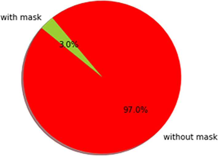
This shows that people not wearing mask has very high risk (97.0%) of getting infected

Fig. 2.

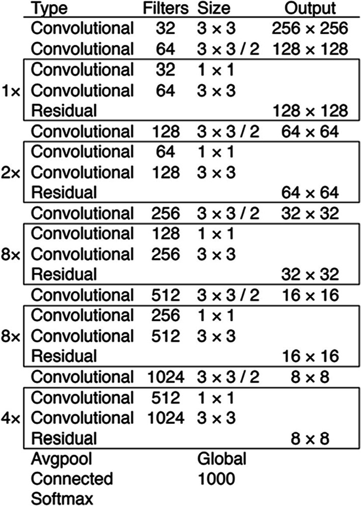
YOLOv3 neural network

The primary contributions of this article are twofold: 1) A method for face mask detection using YOLO and faster R-CNN models. 2) A comprehensive survey on the key difficulties in face mask detection, which might be useful for developing new face mask detectors in the future. Transfer learning is used for making the models in this article. It is a machine learning method where a model developed for some task is reused as the starting point for a model on a related task. It is a popular approach in deep learning where pre-trained models are used as the starting point in computer vision and natural language processing tasks, given the vast computational and time resources required to develop neural network models from the root of these problems and the huge jumps in a skill that they provide on related problems [4]. YOLOv3 and Faster R-CNN are the two algorithms used by authors for making models and a comparison is also done between their results. Faster R-CNN has two networks: A Region proposal network (RPN) [7] for generating region proposals and a network using these proposals to detect objects. RPN ranks region boxes (called anchors) and proposes the ones most likely containing objects. YOLO is a clever convolutional neural network (CNN) for doing object detection in real-time. The algorithm applies a single neural network to the full image, and then divides the image into regions and predicts bounding boxes and probabilities for each region [6]. It becomes very difficult to train these models, keeping in mind the diversity of camera angles in images and mask types, so this issue pops out as a challenge for us. Another challenge the authors faced was the unavailability of a large dataset for training the two categories- one with mask and the second without mask, so the authors have made a custom dataset and used transfer learning to achieve this task.

Section 2 of this paper brief us about all the major-related work that has been done in the field of object detection using CNN and RPN based algorithms. Section 3 contains the work proposed by the authors. In this section, they have thoroughly explained YOLOv3 and Faster-RCNN and how these algorithms are used in the development of face mask detection models. Section 4 contains the experimental results and in this section, the authors have tried to compare the performance of models developed using both algorithms. In section 5, the authors have concluded their work and discussed the necessity of this study. In section 6, the authors have discussed the future scope where these models can be deployed and used in real-world scenarios.

Related work

Whenever there are multiple objects in an image or frame of the video and we want to localize and classify them all, we look for an object detection algorithm. Over the decade, lots of algorithms and techniques have been developed for object detection. YOLO and faster-RCNN are among them and have found their applications in defense systems. Militaries have started to use them along with surveillance cameras for enhancing security. Advanced automobiles like Tesla completely rely on these object detection algorithms for the very concept of self-driving cars. In this section, the authors will be throwing light on these two algorithms.

YOLO algorithm

Image classification using CNN

CNN plays an important role in computer vision related pattern recognition tasks, because of its superior spatial feature extraction capability and less computation cost [1]. One of its very useful applications is a binary classification of images. CNN uses convolution kernels to convolve with the original images or feature maps to extract higher-level features. However, how to design better Convolutional neural network architectures remains an opening question. Inception network is one of the most widely used and accepted convolutional neural network proposed in [9]. It allows the network to learn the best combination of kernels. In order to train much deeper neural networks, Residual Network (ResNet) [2] was proposed, which can learn an identity mapping from the previous layer. As object detectors are usually deployed on mobile or embedded devices, where the computational resources are very limited, Mobile Network (MobileNet) [3] was proposed. It uses depth-wise convolution to extract features and channel-wise convolutions to adjust channel numbers, so the computational cost of MobileNet is much lower than the networks using standard convolutions.

In CNN’s, we take a small matrix of numbers (called kernel or filter), pass it over our image, and transform it based on the values from the filter. Subsequent feature map values are calculated according to the following formula, where the input image is denoted by f and our kernel by h. The indexes of rows and columns of the result matrix are marked with m and n respectively.

$$G\left[m,n\right]=\left(f\times h\right)\left[m,n\right]={\Sigma }_j{\Sigma }_{i}h\left[j,k\right]f\left[m-j,n-k\right]$$

Since our image shrinks every time, we perform convolution, we can do it only a limited number of times before our image disappears completely. What’s more, if we look at how our kernel moves through the image, we see that the impact of the pixels located on the outskirts is much smaller than those in the center of the image. So, we can pad our image with an additional border. The padding width should meet the following equation, where p is padding and f is the filter dimension

$$P=\left(f-1\right)/2$$

Instead of shifting the kernel by one pixel, we can increase the number of steps. So, step length is also treated as one of the convolution layer hyperparameters. The dimensions of the output matrix taking into account both padding and stride - can be calculated using the following formula.

$$n\text{out}=\mathit{\text{floor}}\left(1+\frac{n+2p-f}{s}\right)$$

The filter and the image you want to apply it to must have the same number of channels. If we want to use multiple filters on the same image, we carry out the convolution for each of them separately, stack the results one on top of the other and combine them into a whole. The dimensions of the received tensor (as our 3D matrix can be called) meet the following equation, in which: n — image size, f — filter size, n_c — number of channels in the image, p —used padding, s — used stride, n_f — number of filters.

$$\begin{array}{cc}\left[n,n,n\mathrm{c}\right]\times \left[f,f,n\mathrm{c}\right]=[\text{floor}& \left(1+\frac{n+2p-f}{s}\right),\mathit{\text{floor}}\left(1+\frac{n+2p-f}{s}\right),\mathit{\text{nf}}]\end{array}$$

During forward propagation, we calculate the intermediate value Z, which is obtained as a result of the convolution of the input data from the previous layer with W tensor (containing filters), and then adding bias b. Then we apply a non-linear activation function to our intermediate value (g).

$$\begin{array}{cc}{\mathrm{Z}}^{\left[\mathrm{l}\right]}={\mathrm{W}}^{\left[\mathrm{l}\right]}.{\mathrm{A}}^{\left[\mathrm{l}-1\right]}+{\mathrm{b}}^{\left[\mathrm{l}\right]}& {\mathrm{A}}^{\left[\mathrm{l}\right]}={\mathrm{g}}^{\left[\mathrm{l}\right]}\left({\mathrm{Z}}^{\left[\mathrm{l}\right]}\right)\end{array}$$

During back propagation, we use the following formulae for calculating derivatives:

$$\begin{array}{ccc}{\mathrm{dA}}^{\left[\mathrm{l}\right]}=& \frac{\mathit{\delta l}}{{\mathit{\delta A}}^{\left[l\right]}}{\mathrm{dZ}}^{\left[\mathrm{l}\right]}=& \begin{array}{cc}\frac{\mathit{\delta l}}{{\mathit{\delta Z}}^{\left[l\right]}}{\mathrm{dW}}^{\left[\mathrm{l}\right]}=& \begin{array}{cc}\frac{\mathit{\delta l}}{{\mathit{\delta W}}^{\left[l\right]}}{\mathrm{db}}^{\left[\mathrm{l}\right]}=& \frac{\mathit{\delta l}}{{\mathit{\delta b}}^{\left[l\right]}}\end{array}\end{array}\end{array}$$

There have been massive developments in the applications of convolutional neural networks. Researchers have come forward to address the problems like RGBD-based detection and categorization of waste objects for nuclear decommissioning using multi-image classifiers [8].

Face mask detectors can also be built by simply using CNNs along with any of the famous architecture like ResNet or inception network and then applying sigmoid activation function at the end on the fully connected dense final layer. This is a really good application when we have only one person in the frame and we have to classify if he/she is wearing a mask or not. It can be used at places like the entrance gate of some institutes, but it cannot detect multiple faces in an image and also cannot draw different colored bounding boxes around the faces. We need to address this problem using object detection models instead.

Object detection using CNN

Image classification refers to assigning a class label to an image. Object localization refers to sketching a bounding box around the object in an image. Object detection is more difficult and blends these two tasks and draws a bounding box around each object of interest in the image and allocates them a class label. Let’s see how simple binary or multi-classification algorithms are modified to draw the bounding boxes around the object. We just change the output labels from the previous algorithm, so as to make our model learn the class of the object and also the position of the object in the image. We add 4 more numbers in the output layer which include the centroid position of the object and the proportion of width and height of the bounding box in the image. This solves the problem of object localization. Now, we want our algorithm to be able to classify and localize all the objects in an image, not just one. So, the idea is to crop the image into multiple images and run CNN for all the cropped images.

First of all, make a window of size much smaller than the actual image size. Crop it and pass it to CNN and have CNN make the predictions. Keep on sliding the window and pass the cropped images into CNN. After cropping all the portions of the image with this window size, repeat all the steps again for a bit bigger window size. Again, pass cropped images into CNN and let it make predictions. In the end, you will have a set of cropped regions which will have some object, together with the class and bounding box of the object. This solution is known as object detection with sliding windows. YOLO algorithm uses this idea for object detection. YOLOv3 uses successive 3 × 3 and 1 × 1 convolutional layer and has some shortcut connections as well. It has 53 convolutional layers.

Faster R-CNN algorithm

Faster R-CNN is most widely used state of the art version of the R-CNN family. These networks usually consist of — a) A region proposal algorithm to generate “bounding boxes” or locations of possible objects in the image. b) A feature generation stage to obtain features of these objects, usually using a CNN. c) A classification layer to predict which class this object belongs to and d) A regression layer to make the coordinates of the object bounding box more precise.

Fast R-CNN used CPU based selective search algorithm for region proposal, which takes around 2 s per image and runs on CPU computation. The Faster R-CNN [7] paper fixes this by using Region Proposal Network (RPN) to generate the region proposals. This not only brings down the region proposal time from 2 s to 10 ms per image but also allows the region proposal stage to share layers with the following detection stages, causing an overall improvement in feature representation.

Region proposal network (RPN)

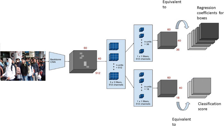
The region proposal network (RPN) starts with the input image being fed into the backbone convolutional neural network. The input image is first resized such that its shortest side is 600px with the longer side not exceeding 1000px. The output features of the backbone network are usually much smaller than the input image depending on the stride of the backbone network. For every point in the output feature map, the network has to learn whether an object is present in the input image at its corresponding location and estimate its size. This is done by placing a set of “Anchors” on the input image for each location on the output feature map from the backbone network. These anchors indicate possible objects in various sizes and aspect ratios at this location. As the network moves through each pixel in the output feature map, it has to check whether these k corresponding anchors spanning the input image actually contain objects, and refine these anchors’ coordinates to give bounding boxes as “Object proposals” or regions of interest (Figs. 3 and 4).

Fig. 3.

RPN architecture

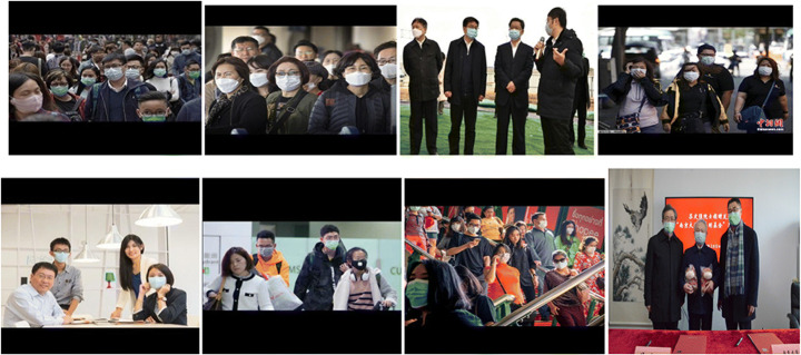
Fig. 4.

Masked faces with diversified orientations, degrees of occlusion and mask types

First, a 3 × 3 convolution with 512 units is applied to the backbone feature map, to give a 512-d feature map for every location. This is followed by two sibling layers: a 1 × 1 convolution layer with 18 units for object classification, and a 1 × 1 convolution with 36 units for bounding box regression. The 18 units in the classification branch give an output of size (H, W, 18). This output is used to give probabilities of whether or not each point in the backbone feature map (size: H × W) contains an object within all 9 of the anchors at that point. The 36 units in the regression branch give an output of size (H, W, 36). This output is used to give the 4 regression coefficients of each of the 9 anchors for every point in the backbone feature map (size: H × W). These regression coefficients are used to improve the coordinates of the anchors that contain objects.

Object detection using RPN and a detector network (fast-RCNN)

The Faster R-CNN architecture consists of the RPN as a region proposal algorithm and the Fast R-CNN as a detector network. Faster R-CNN tries to find out the areas that might be an object by combining similar pixels and textures into several rectangular boxes. The simple R-CNN used 2000 proposed areas (rectangular boxes) from search selective. But, fast R-CNN was a significant improvement because instead of applying 2000 times CNN to the proposed areas, it only passes the original image to a pre-trained CNN model once. Faster R-CNN makes further progress than Fast R-CNN. Search selective process is replaced by Region Proposal Network (RPN).

The input image is first passed through the backbone CNN to get the feature map (Feature size: 60, 40, 512). Besides test time efficiency, another key reason using an RPN as a proposal generator makes sense is the advantages of weight sharing between the RPN backbone and the Fast R-CNN detector backbone. Next, the bounding box proposals from the RPN are used to pool features from the backbone feature map. This is done by the ROI pooling layer. The ROI pooling layer, in essence, works by a) Taking the region corresponding to a proposal from the backbone feature map; b) Dividing this region into a fixed number of sub-windows; c) Performing max-pooling over these sub-windows to give a fixed size output. To understand the details of the ROI pooling layer and it’s advantages, read Fast R-CNN. The output from the ROI pooling layer has a size of (N, 7, 7, 512) where N is the number of proposals from the region proposal algorithm. After passing them through two fully connected layers, the features are fed into the sibling classification and regression branches. These classification and detection branches are different from those of the RPN. Here the classification layer has C units for each of the classes in the detection task (including a catch-all background class). The features are passed through a soft-max layer to get the classification scores — the probability of a proposal belonging to each class. The regression layer coefficients are used to improve the predicted bounding boxes.

From the above descriptions of both algorithms, it can be seen that faster R-CNN’s input goes under a lot of work before finally sending the image to the detector network. Whereas in YOLOv3, localization and classification processes, both happen in a single network. So, as expected, YOLOv3 is much faster than Faster R-CNN but the quality of faster R-CNN output is indeed greater than YOLO’s output. It can detect finer details. There is a compromise between quality and speed here. But we will see that this becomes insignificant in real-time object detection because, in deployed models, it becomes very important to detect quickly, and also a difference in output’s quality is very small.

Proposed work

Many people have come up with creative ideas for detecting face-masks (like putting artificial mask images on top of non-mask people images) but the authors found that most of them solved this issue using simple CNN models considering it as a binary classification problem. This problem needs to be handled using object detection models for detecting multiple people in the frame, then putting bounding boxes of particular colour around them depending on whether they are wearing masks or not, and analysing the ratio of people wearing masks. There was a need for a dataset with labels and annotations. So, the authors have generated a small custom dataset manually, carefully provided labels, and used transfer learning to achieve this task. They have also used some datasets available on the web and provided their description. We trained both our models on the same dataset of ~7500 images. Each face in every image was labelled with carefully prepared bounding boxes. Annotation records containing all the data about bounding boxes, image names, and labels are prepared in the various formats as required by both the models considered in this work. The dataset is composed of MAFA, WIDER FACE (http://shuoyang1213.me/WIDERFACE/) and many manually prepared images by surfing various sources on the web and is made accessible along with the annotation records in the following link:

https://drive.google.com/drive/folders/1pAxEBmfYLoVtZQlBT3doxmesAO7n3ES1?usp=sharing

Keras API has been used by the authors on top of the TensorFlow machine learning library in python for implementation of both the models because Keras supports almost all the models of a neural network – fully connected, convolutional, pooling, recurrent, embedding, etc. Furthermore, these models can be combined to build more complex models. The final models obtained after training and validation are made accessible by the authors. They are in ‘.h5’ file format which is a grid format that is ideal for storing multi-dimensional arrays of numbers and is supported by Keras only.The model shared by authors can be loaded by public using the load_model() function and passing the filename. The function returns the model with the same architecture and weights as obtained by authors after a lot of training and validation.

YOLO v3

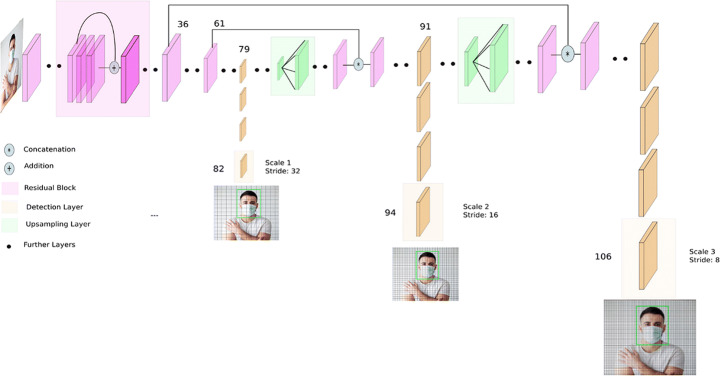
If one can look at the architecture of YOLOv3, it contains 53 convolutional layers, trained on ImageNet. For the task of detection, 53 more layers are stacked onto it, giving us a 106 layer fully convolutional underlying architecture for YOLO v3. In YOLO v3, the detection is done by applying detection kernels on feature maps of three different sizes at three different places in the network.

The shape of the detection kernel is 1 × 1 × (B×(5 + C)). Here B is the number of bounding boxes a cell on the feature map can predict, “5” is for the 4 bounding box attributes and one object confidence, and C is the number of classes. In YOLO v3, B = 3 and C = 80, so the kernel size is 1× 1× 255. The first detection is made by the 82nd layer. For the first 81 layers, the image is down-sampled by the network, such that the 81st layer has a stride of 32. If we have an image of 416 × 416, the resultant feature map would be of size 13 × 13. One detection is made here using the 1 × 1 detection kernel, giving us a detection feature map of 13 × 13 × 255. Then, the feature map from layer 79 is subjected to a few convolutional layers before being upsampled by 2× to dimensions of 26 × 26. This feature map is then depth concatenated with the feature map from layer 61. Then the combined feature maps are again subjected to a few 1 × 1 convolutional layer to fuse the features from the earlier layer (61). Then, the second detection is made by the 94th layer, yielding a detection feature map of 26 × 26 × 255. A similar procedure is followed again, where the feature map from layer 91 is subjected to few convolutional layers before being depth concatenated with a feature map from layer 36. Like before, a few 1 × 1 convolutional layer follow to fuse the information from the previous layer (36). We make the final of the 3 at the 106th layer, yielding a feature map of size 52 × 52 × 255.

Detections at different layers help address the issue of detecting small objects found in its predecessor YOLO v2. The complete architecture of YOLOv3 is depicted in Fig. 5.

Fig. 5.

Yolov3 architecture

For the task of face-mask detection, the authors initially trained this model on their facemask dataset keeping the final 3 layers unfrozen and later trained the complete model for fine-tuning the weights. The 9 anchors they used are the ones used by the pre-trained model.

Pseudocode

Training:

1. Generate your own annotation file and class names file:

   Row Format: image_file_path box 1, box2, ... boxN.

   Box format: x_min, y_min, x_max, y_max, class_id

2. Convert the pre-trained weights to ‘.h5’ format as required by Keras.

3. Freeze all layers except the final layers and train for some epochs until Plateau (no improvement stage) is reached.

4. Unfreeze all the layers and train all the weights while continuously reducing the learning rate until again plateau is reached.

5. End

Testing on webcam or video in keras using OpenCV:

1. Capture the video through webcam or any saved video testing file.

2. Pass each frame of video or captured frame from webcam through the model.

3. Get the boxes, scores and classes obtained as output and draw the boxes on the frame accordingly (colour depending on the class of each box).

4. Display a total number of boxes of both classes at the bottom of the screen and record them in a variable.

5. After iterating through each frame, we shall be able to get the output video with the results we wanted.

Training of YOLO v3

For training the YOLO v3 model, we took the weights of a pre-trained model as our starting point. We used the weights provided by original author Joseph Redmon on his website- https://www.pjreddie.com. We froze all the layers except the last 3 layers of the model and trained it for ~70 epochs on the dataset. After that model was tested on some videos, but the result was not very satisfactory as we had not fine-tuned the model. For fine tuning of the model, unfreezing of all the layers of our model was done and we trained it for some more epochs. After reducing the learning rate, a couple of times, we were able to get some satisfactory results. In Fig. 6, the authors have presented the results of the YOLOv3 model. In this case, the thresholds used for IOU and score are 0.5 and 0.4, respectively. Here are the weights obtained after training for a decent amount of time: https://drive.google.com/file/d/1-zQ1aV5phEGPJauaJ6Z9Go8VndmDT170/view?usp=sharing

Fig. 6.

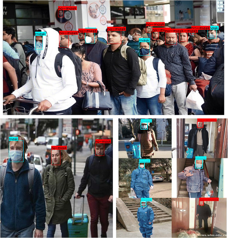
Results from YOLO_v3 model

Model parameters can be further optimized by retraining this already trained model on some new dataset. Instead of keeping the weights of pre-trained models (provided by the original author- Joseph Redmon) as the starting point, if one uses the weights we obtained as the starting point, further optimized parameters can be obtained.

Final values of loss we obtained after ~63 epochs (plateau was reached) are:

• Training loss- 0.1.

• Validation loss- 0.25.

Faster-RCNN

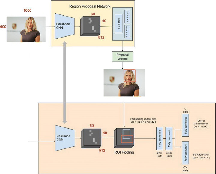
The architecture of faster R-CNN is a simple convolution layer with kernel size 3 × 3 followed by a regional proposal network (RPN) and then a detector network. The input image is first resized such that its shortest side is 600px with the longer side not exceeding 1000px and passed through the RPN network. After passing through RPN, we get an output feature map with a significantly smaller size from the input. If the input image has 600 × 800 × 3 dimensions, the output feature map would be 37 × 50 × 256 dimensions. Two consecutive pixels in the backbone output features correspond to two points 16 pixels apart in the input image. Each point in 37 × 50 is considered as an anchor.

Next, RPN is connected to a Conv layer with 3 × 3 filters, 1 padding, 512 output channels. The output is connected to two 1 × 1 convolutional layer for classification and box-regression. Every anchor has 3 × 3 = 9 corresponding boxes in the original image, which means there are 37 × 50 × 9 = 16,650 boxes in the original image. We just choose 256 of these 16,650 boxes as a mini-batch which contains 128 foregrounds (pos) and 128 backgrounds (neg). At the same time, non-max suppression is applied to make sure there is no overlapping for the proposed regions.

Then we go to the second stage of frcnn. Similar to Fast R-CNN, ROI pooling is used for these proposed regions (ROIs). The output is 7 × 7 × 512. Then, we flatten this layer with some fully connected layers. The final step is a soft-max function for classification and linear regression to fix the boxes’ location.

The architecture of faster-RCNN is shown in Fig. 7.

Fig. 7.

Faster-RCNN architecture

Again, in this case, thresholds used for IOU and score are 0.5 and 0.4, respectively.

Training of faster-RCNN

Pseudocode

Training of Faster R-CNN:

1. Put training and validation images in separate train_images and test_images folders.

2. Generate train.csv annotation file and class names file: -

   Row Format: image_file_path,x_min,y_min,x_max,y_max,class_name.

   Note that in the case of F-RCNN, all boxes of the image are not written in a single row. Each box is written on a different row and we must write class name instead of class id unlike YOLOv3 format.

3. We need to convert the .csv format into a .txt file which will have the same format as described above. Make a new data frame, fill all the values as per the format into that data frame, and then save it as a .txt file.

4. onvert the pre-trained weights to ‘.h5’ format as required by Keras.

5. Unfreeze all the layers and train all the weights while continuously reducing the learning rate until a plateau is reached and loss is low and constant for both validation and training dataset.

Pseudo code for testing on webcam or video in Keras using OpenCV:

1. Capture the video through the webcam or any saved video testing file.

2. Pass each frame of video or captured frame from the webcam through the model.

3. Define the threshold for IOU and scores.

4. Get the boxes, scores and transform the coordinates of the bounding boxes to their original size.

5. Draw coloured rectangles in place of coordinates and display a total number of boxes of both classes at the bottom of the screen and record them in a variable.

6. After iterating through each frame, we shall be able to get the output video with the results we wanted.

For training the Faster-RCNN model, the authors used ResNet-101-FPN architecture as the backbone for the base model. They used pre-trained weights provided by facebook’s model zoo as the starting point and trained all the layers for ~50 epochs on their dataset while reducing the learning rate occasionally. The same dataset is considered for experimental work which is used for experimental work with the YOLO v3 model.

Final results of faster R-CNN

In faster R-CNN, there were two loss functions that we applied to both the RPN model and Classifier model. They both showed a similar tendency and even similar loss value while training. The total loss i.e., the sum of both the losses had a decreasing tendency. Total training loss we obtained after ~50 epochs was 0.04 and total validation loss was 0.15.

It would be better if we could analyze the percentage of people wearing masks on a daily basis. For this task, both the models (YOLOv3 and FRCNN) are modified in such a way that the algorithm is tested on videos. For each frame of video, we calculated the ratio of people wearing masks and record it. After testing each frame of the video, we convert the new frames back to a video and take the average of all ratios to analyze the number of people wearing masks on a daily basis.

Experimental results

After testing a significant number of videos, we found that the accuracy of both the models is good but F-RCNN is marginally better. F-RCNN has a place with the RCNN family and falls under the two-phase identifier’s classification. The procedure contains two phases. To start with, we obtain region proposals and afterward classify each proposal and predict the bounding box. These detectors normally lead to great identification accuracy yet the interpretation time of these detectors with region proposals require massive computation and run-time memory, whereas, detectors having a place with the YOLO series fall under single stage detectors. It is a solitary stage process. These models use the predefined stays that cover spatial position, scales, and aspect ratios across an image. Hence, we do not need an additional branch for separating the area proposition. Since all computations are in a solitary system, they are bound to run quicker than the two-phase detectors. YOLOv3 is also a single-stage detector and at present the state-of-the-art for object detection. For a rough comparison of these two object detection models, we calculated the Average Precision by taking IOU = 0.5 for both the models on some examples and got the following results (Table 1).

Table 1.

Comparative analysis

MODEL	Average Precision	Inference Time
YOLOv3	55	0.045 s
Faster R-CNN	62	0.15 s

So, from our results, both our models are fairly accurate but for applying these models in real-world surveillance cameras or other real-world applications, it would be preferable to use the model with the YOLOv3 algorithm as it performs single-shot detection and has much less inference time than Faster-RCNN or any other state-of-the-art object detection algorithms though there is some trade-off between speed and precision. Let us take the case of self-driving vehicles. Consider that we have trained an object identification model that takes a couple of moments to recognize objects in an image and we employed this model in a self-driving vehicle. We positively might not want to see such a model in action! The inference time here is excessive. The vehicle will set aside a great deal of effort to settle on choices that may prompt significant circumstances like mishaps too. Hence, in such situations, we need a model that will give us real-time results. Experimental results of both models, namely, YOLOv3 and Faster-RCNN are depicted in Figs. 6 and 8, respectively.

Fig. 8.

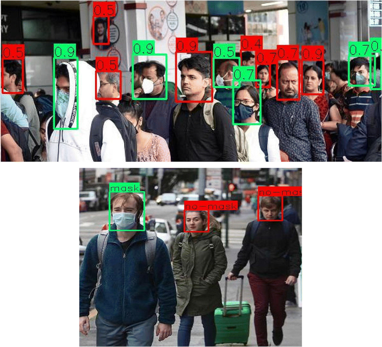
Results from faster-RCNN model

Conclusion

The article proposed an efficient real-time deep learning-based technique to automate the process of detecting masked faces, where each masked face is identified in real-time with the help of bounding boxes. The extensive trials were conducted with popular models, namely, Faster RCNN and YOLO v3. F-RCNN has better precision, but for applying this in real-world surveillance cameras, it would be preferred to use the model with YOLO algorithm as it performs single-shot detection and has a much higher frame rate than Faster-RCNN or any other state-of-the-art object detection algorithms. If we look at the speed/accuracy tradeoff on the mAP at .5 IOU metric, one can tell YOLOv3 is better than faster R-CNN. Which model to use, also depends on the resources available. If high-end GPUs are available on the deployed devices, faster R-CNN must be used. YOLOv3 can be deployed on mobile phones also. Since this approach is highly sensitive to the spatial location of the camera, the same approach can be fine-tuned to better adjust with the corresponding field of view. These models can be used along with surveillance cameras in offices, metros, railway stations and crowded public areas to check if people are following rules and wearing marks. The trained weights provided by the authors can be further improved by training on larger datasets and can then be used in real-world applications.

Future scope

This application can be used in any working environment like any public place, station, corporate environment, streets, shopping malls, examination centers, etc., where accuracy and precision are highly desired to serve the purpose. This technique can be used in smart city innovation and it would boost up the development process in many developing countries. Our analysis of the current circumstance presents a chance to be more ready for the next crisis, or to evaluate the effects of huge scope social change.

Declarations

Competing interests

The authors declare that they have no known competing financial interests or personal relationships that could have appeared to influence the work reported in this paper.

References

- 1.Deng J, Dong W, Socher R, Li L-J, Li K, Fei-Fei L (2009) Imagenet: A large-scale hierarchical image database. Proceedings of IEEE Conference on Computer Vision and Pattern Recognition, pp 248–255
- 2.He K, Zhang X, Ren S, Sun J (2016) Deep residual learning for image recognition. Proceedings of IEEE Conference on Computer Vision and Pattern Recognition, pp 770–778
- 3.Howard AG, Zhu M, Chen B, Kalenichenko D, Wang W, Weyand T, Andreetto M, Adam H (2017) Mobilenets: efficient convolutional neural networks for mobile vision applications. arXiv preprint arXiv:1704.04861, 2017
- 4.Jason B A Gentle Introduction to Transfer Learning for Deep Learning. https://machinelearningmastery.com/transfer-learning-for-deep-learning/
- 5.Matuschek C, Moll F, Fangerau H, Fischer JC, Zänker K, van Griensven M, Schneider M, Kindgen-Milles D, Knoefel WT, Lichtenberg A, Tamaskovics B, Djiepmo-Njanang FJ, Budach W, Corradini S, Häussinger D, Feldt T, Jensen B, Pelka R, Orth K, Peiper M, Grebe O, Maas K, Gerber PA, Pedoto A, Bölke E, Haussmann J. Face masks: benefits and risks during the COVID-19 crisis. Eur J Med Res. 2020;25:32. doi: 10.1186/s40001-020-00430-5. [DOI] [PMC free article] [PubMed] [Google Scholar]
- 6.Redmon J, Divvala S, Girshick R, Farhadi A (2016) You only look once: unified, real-time object detection, vol 2016. IEEE Conference on Computer Vision and Pattern Recognition (CVPR), Las Vegas, pp 779–788. 10.1109/CVPR.2016.91
- 7.Shaoqing R, Kaiming H, Girshick R, Jian S. Faster R-CNN: towards real-time object detection with region proposal networks. IEEE Trans Pattern Anal Mach Intell. 2015;39:1137–1149. doi: 10.1109/TPAMI.2016.2577031. [DOI] [PubMed] [Google Scholar]
- 8.Sun L, Zhao C, Yan Z, Liu P, Duckett T, Stolkin R. A novel weakly-supervised approach for RGB-D-based nuclear waste object detection. IEEE Sensors J. 2019;19:3487–3500. doi: 10.1109/JSEN.2018.2888815. [DOI] [Google Scholar]
- 9.Szegedy C, Liu W, Jia Y, Sermanet P, Reed S, Anguelov D, Erhan D, Vanhoucke V, Rabinovich A (2015) Going deeper with convolutions. Proceedings of IEEE Conference on Computer Vision and Pattern Recognition, pp 1–9
- 10.W H Organization (2020) WH corona-viruses (COVID-19),” https://www.who.int/emergencies/diseases/novel-corona-virus-2019