Optimal Immunity Control and Final Size Minimization by Social Distancing for the SIR Epidemic Model

Abstract

The aim of this article is to understand how to apply partial or total containment to SIR epidemic model during a given finite time interval in order to minimize the epidemic final size, that is the cumulative number of cases infected during the complete course of an epidemic. The existence and uniqueness of an optimal strategy are proved for this infinite-horizon problem, and a full characterization of the solution is provided. The best policy consists in applying the maximal allowed social distancing effort until the end of the interval, starting at a date that is not always the closest date and may be found by a simple algorithm. Both theoretical results and numerical simulations demonstrate that it leads to a significant decrease in the epidemic final size. We show that in any case the optimal intervention has to begin before the number of susceptible cases has crossed the herd immunity level, and that its limit is always smaller than this threshold. This problem is also shown to be equivalent to the minimum containment time necessary to stop at a given distance after this threshold value.

Introduction

The current outbreak of Covid-19 and the entailed implementation of social distancing on an unprecedented scale led to renewed interest in modeling and analysis of this method to control infectious diseases. In contrast with a recent trend of papers that aim at giving a large account of the complexity of the pandemic, in its epidemiological dimension, but also from the point of view of the functioning of the hospital and public health systems, and even possibly the behavioral aspects, our perspective here is quite different. Our purpose is to study, at a theoretical level, how to use social distancing in an optimal way, in order to minimize the cumulative number of cases infected during the course of an epidemic. This issue is addressed in the framework of the classical SIR model, in line with other papers that studied optimal epidemic control, through treatment, vaccination, quarantine, isolation or testing. This simplified setting deliberately ignores many features important in the effective handling of a human epidemic: population heterogeneity, limited hospital capacity, imprecision of the epidemiological data (including the question of the asymptomatic cases), partial respect of the confinement, etc. On the other hand, thanks to its simplicity complete, computable, solutions are achievable to serve as landmark for real situations. In a nutshell, our aim is to determine what best result may be obtained in terms of reduction of the total cumulative number of infected individuals by applying lockdown of given maximal intensity and duration, in the worst conditions where no medical solution is discovered to stop earlier the epidemic spread.

The SIR model is described by the following system, in which all parameters are positive:

$$\begin{array}{cc}\hfill \dot{S}=& -\beta SI,S(0)=S_0,\hfill \end{array}$$ 1a

$$\begin{array}{cc}\hfill \dot{I}=& \beta SI-\gamma I,I(0)=I_0,\hfill \end{array}$$ 1b

$$\begin{array}{cc}\hfill \dot{R}=& \gamma I,R(0)=R_0.\hfill \end{array}$$ 1c

The state variables S, I and R correspond, respectively, to the proportions of susceptible, infected and removed individuals in the population. The sum of the derivatives of the three state variables is zero, so the sum of the variables remains equal to 1 if initially $S_0+I_0+R_0=1$, and one may describe the system solely with Eqs. (1a)–(1b). The total population is constant and no demographic effect (births, deaths) is modeled, as they are not relevant to the time scale to be taken into account in reacting to an outbreak. The infection rate $\beta$ accounts globally for the rate of encounters between the individuals and the probability of transmitting the infection during each of these encounters. The parameter $\gamma$ is the recovery rate. Recovered individuals are assumed to have acquired permanent immunity.

Obviously, every solution of (1) is nonnegative, and thus, $\dot{R}⩾0⩾\dot{S}$ at any instant, so S and $S+I$ decrease, while R increases. We infer that every state variable admits a limit and that the integral ${\int }_0^{+\infty }\beta I(t)dt$ converges. Therefore,

$$\begin{array}{c}\hfill \underset{t\to +\infty }{lim}I(t)=0,S_{\infty }:=\underset{t\to +\infty }{lim}S(t)>0\text{if}{S}_0>0.\end{array}$$ 2

The basic reproduction number ${\mathcal{R}}_0:=\beta /\gamma$ governs the behavior of the system departing from its initial value. When ${\mathcal{R}}_0<1$, $\dot{I}=(\beta S-\gamma )I$ is always negative: I decreases and no epidemic may occur. When ${\mathcal{R}}_0>1$ epidemic occurs if $S_0>\frac{1}{{\mathcal{R}}_0}$. In such a case, I reaches a peak and then goes to zero. From now on, we assume

$$\begin{array}{c}\hfill {\mathcal{R}}_0=\frac{\beta }{\gamma }>1.\end{array}$$

An important issue is herd immunity. The latter occurs naturally when a large proportion of the population has become immune to the infection. Mathematically, it is defined as the value of S below which the number of infected decreases. For the SIR model (1), one has $\dot{I}=(\beta S-\gamma )I$, and

$$\begin{array}{c}\hfill S_{\mathrm{herd}}:=\frac{\gamma }{\beta }=\frac{1}{{\mathcal{R}}_0}.\end{array}$$ 3

Notice that, after passing the collective immunity threshold, that is for large enough t, one has

$$\begin{array}{c}\hfill S_{\mathrm{herd}}⩾S(t)⩾S_{\infty }.\end{array}$$ 4

While the number of infected decreases when $S(·)⩽S_{\mathrm{herd}}$, epidemics continue to consume susceptible and to generate new infections once the immunity threshold has been crossed. The number of infected cases appearing after this point may be quite large. In order to illustrate this fact, Table 1 displays, for several values of ${\mathcal{R}}_0$, the value of the herd immunity threshold and the number of susceptibles that remain after the fading out of the outbreak, in the case of an initially naive population ($S_0\approx 1$). The proportion of infections occurred after the overcome of the immunity is also shown.

Table 1.

Herd immunity level $S_{\mathrm{herd}}$ and asymptotic susceptible proportion $S_{\infty }$ for initial value $S_0\approx 1$ for several values of the basic reproduction number ${\mathcal{R}}_0$

${\mathcal{R}}_0$	1.5	2	2.5	2.9	3	3.5
$S_{\mathrm{herd}}$	0.67	0.50	0.40	0.34	0.33	0.29
$S_{\infty }$	0.42	0.20	0.11	0.067	0.059	0.034
${\displaystyle \frac{S_{\mathrm{herd}}-S_{\infty }}{1-S_{\infty }}}$	43%	37%	33%	30%	29%	27%

The value of $S_{\mathrm{herd}}$ comes from (3), and $S_{\infty }$ may be deduced from the fact that $S_{\infty }-\frac{1}{{\mathcal{R}}_0}ln{S}_{\infty }\approx 1$, see Lemma 4.2 below. The ratio $\frac{S_{\mathrm{herd}}-S_{\infty }}{1-S_{\infty }}$ represents the proportion of susceptible that occur after passing the collective immunity threshold. The column in bold corresponds to ${\mathcal{R}}_0$ found in [39] for the SARS-CoV-2 in France before the lockdown of March–May 2020

Apart from medical treatment, there are generally speaking three main methods to control human diseases. Each of them, alone or in conjunction with the others, gave rise to applications of optimal control. A first class of interventions consists in vaccination or immunization [2, 4, 8, 10, 11, 14, 16–18, 20, 30, 37, 40, 43]. It consists in transferring individuals from the S compartment to the R one. The members of the latter may not be stricto sensu recovered: they are removed from the infective process. A second class of measures corresponds to screening and quarantining of infected [1, 3, 8, 10, 11, 41, 42, 44]. It may be modeled by transfer of individuals from the I compartment to the R one (which consequently will change its meaning). Last, it is possible to reduce transmission through health promotion campaigns or lockdown policies [8, 10, 34, 36]. Of course these methods may be employed jointly [18].

Other modeling frameworks have also been considered. More involved models called SEIR and SIRS have been analyzed in [8, 16], and SIR model structured by the infection age in [3]. Constraints on the number of infected persons that the public health system can accommodate or on available resources, particularly in terms of vaccination, were studied [10, 11, 34, 43, 44]. Economical considerations may be aggregated to the epidemiological model [5, 29, 38]. Ad hoc models for tackling emergence of resistance to drugs issues have been introduced [22, 23], as well as framework allowing to study revaccination policies [27, 28]. Optimization of vaccination campaigns for vector-borne diseases has also been considered [40]. Optimal public health intervention as a complement to such campaigns has been studied in [12, 13] (see [33] for more material on behavioral epidemiology). The references cited above are limited to deterministic differential models, but discrete-time models and stochastic models have also been used, e.g., in [1, 2, 17].

The costs considered in the literature are usually integral costs combining an “outbreak size” (the integral of the number of infected, or of the newly infected term, or the largest number of infected) and the input variable on a given finite time horizon. Some minimal time control problems have also been considered [4, 10, 11, 21]. The integral of the deviation between the natural infection rate and its effective value due to confinement is used in [34], together with constraints on the maximal number of infected. In [7], the authors minimize the time needed to reach herd immunity, under the constraint of keeping the number of infected below a given value, in an attempt to preserve the public health system. Few results consider infinite horizon [8]. Qualitatively, optimal solutions attached to the vaccination or isolation protocols are in general bang-bang,1 with an intervention from the very beginning. Bounds on the number of switching times between the two modes (typically zero or one) are sometimes provided. By contrast, protocols that mitigate the transmission rate (health promotion campaigns or lockdown policies) usually provide bang-bang optimal solutions with transmission reduction beginning after a certain time. Generally speaking, there exists no ideal strategy, and the achievement of some policy objective may preclude success with others [19].

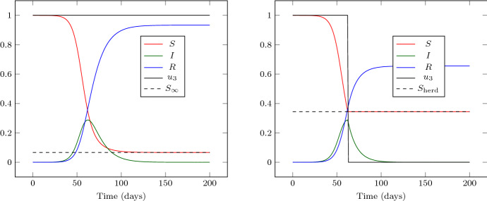
The present article is dedicated to the optimal control issue of obtaining, by enforcing social distancing, the largest value for $S_{\infty }$, the limit number of susceptible individuals at infinity. Using classical vocabulary of epidemiology, this is equivalent to minimize the attack ratio $1-S_{\infty }$ or its unnormalized counterpart, the final size of the epidemic. Abundant literature exists concerning this quantity, since Kermack and Mc Kendrick’s paper from 1927 [25], see, e.g., [6, 24, 32, 35] for important contributions to its computation in various deterministic settings. Said otherwise, we seek here to determine how close to the herd immunity threshold it is possible to stop the spread of a disease, in the case where no vaccine or treatment is found to modify its evolution. A possible action is to let the proportion of susceptible reach the collective immunity level and then impose total lockdown, putting $\beta =0$ in (1) after a certain time. This situation is illustrated in Fig. 1. Merely as a reference point, we use the figures of the Covid-19 in France in Spring 2020, borrowed from [39] and given in Table 2. In this way one may stop exactly at the herd immunity threshold; however, this is achieved by applying total lockdown during infinite time duration (Fig. 2).

Fig. 1.

Numerical simulation of the SIR model with the numerical parameters given in Table 2. Left: no action. Right: switch at the epidemic peak ($\beta$ is put to 0 at $t=62$ days)

Table 2.

Value of the parameters used for system (1a)–(1b) (see [39])

Parameter	Name	Value
$\beta$	Infection rate	0.29
$\gamma$	Recovery rate	0.1
${\alpha }_{\text{lock}}$	Lockdown level (France, March/May 2020)	0.231
$S_0$	Initial proportion of susceptible	$1-I_0$
$I_0$	Initial proportion of infected	$1.49\times {10}^{-5}$
$R_0$	Initial proportion of removed	0

Fig. 2.

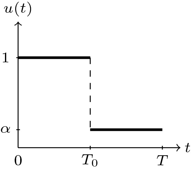
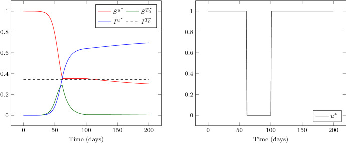
The optimal control belongs to a family of bang-bang functions $u_{T_0}$ parameterized by the switching time $T_0$ represented here

On the contrary, our aim here is to focus more realistically on interventions taking place on a given finite time interval, through possibly partial lockdown. A closely related issue is studied in [26], where only total lockdown is considered.2 Our perspective is slightly different here, as we are equally interested by enforcement measures inducing partial contact reduction. In [15] the authors explore by thorough numerical essays conducted on SIR model the impact of one-shot lockdowns of given intensity and duration, initiated when $S(t)+I(t)$ reaches a certain threshold, with regard to three quantities of interest: the final size, the peak prevalence and the average time of infection. Prolonging the work of the present article, [9] analyzes how to optimally choose the onset of such one-shot interventions, with the aim of maximizing the epidemic final size.

For better readability, all results are exposed in Sect. 2. It is first shown in Sect. 2.1 (Proposition 2.1) that, for strong enough lockdown measures and long enough intervention time T, one can stop the epidemics arbitrarily close after the herd immunity is attained. In Sect. 2.2, we provide and analyze the optimal control law that leads asymptotically, through an intervention of duration T, to the largest number of susceptible individuals. Theorem 2.2 establishes existence and uniqueness of the solution to the optimal control problem, which is bang-bang with a unique commutation from the nominal value to the minimal allowed value of the transmission rate. Theorem 2.3 characterizes in a constructive way the time of this commutation and situates the latter with respect to the peak of the epidemic, and the corresponding proportion of susceptible with respect to the herd immunity level. Last, we show in Sect. 2.3 (Theorem 2.4) that this optimal strategy coincides with a time minimal policy. The results are numerically illustrated in Sect. 3. For the sake of readability, all the proofs are postponed to Sect. 4. Concluding remarks are given in Sect. 5. Last, details on implementation issues are provided in Appendix A.

Notice that from a technical point of view, the problem under study is by nature an optimal control problem on an infinite horizon, as it aims to maximize the limit $S_{\infty }$ of the proportion of susceptible cases. However, by using a quantity invariant along the trajectories (see end of Sect. 2.1 and Lemma 4.2 in Sect. 4.1), one is able to formulate the problem over a finite time horizon, thereby allowing for easier handling.

Main Results

According to the introduction in the previous section, we consider in the sequel the following “SIR type” system

$$\begin{array}{c}\hfill \begin{array}{cc}\dot{S}(t)=-u(t)\beta S(t)I(t),\hfill & t⩾0\hfill \\ \dot{I}(t)=u(t)\beta S(t)I(t)-\gamma I(t),\hfill & t⩾0\hfill \end{array}\end{array}$$ 5

complemented with nonnegative initial data $S(0)=S_0$, $I(0)=I_0$ such that $S_0+I_0⩽1$. The time-varying input control u models public interventions on the transmission rate by measures like social distancing, restraining order, lockdown, and so on, imposed on finite time horizon. For given $T>0$ and $\alpha \in [0,1)$, u is assumed to belong to the admissible set ${\mathcal{U}}_{\alpha ,T}$ defined by

$$\begin{array}{c}\hfill {\mathcal{U}}_{\alpha ,T}:=\{u\in L^{\infty }([0,+\infty )),\alpha ⩽u(t)⩽1\text{if}t\in [0,T],u(t)=1\text{if}t>T\}.\end{array}$$

The constant T characterizes the duration of the intervention, and $\alpha$ its maximal intensity (typically the strength of a lockdown procedure). Admittedly, u represents here a rather abstract quantity: it quantifies how much the nonpharmaceutical measures reduce the rate of contact between susceptible and infected individuals. In practice, though, it would be quite difficult to measure its value, or to assign it a prescribed value. On the other hand, as seen later in Theorem 2.2, the optimal control follows an “all or nothing” pattern: it takes on only the two extreme values, which correspond to stronger possible lockdown or no lockdown at all, so that a precise tuning is not requested in effect.

Toward an Optimal Control Problem: Reachable Asymptotic Immunity Levels

The following result assesses the question of stopping the evolution exactly at, or arbitrarily close to, the herd immunity $S_{\mathrm{herd}}$ defined by (3).

Theorem 2.1

Let $\alpha \in [0,1)$ and $T>0$. Assume that $S_0>S_{\mathrm{herd}}$ and consider

$$\begin{array}{c}\hfill \overline{\alpha }:=\frac{S_{\mathrm{herd}}}{S_0+I_0-S_{\mathrm{herd}}}\left(ln,S_0,-,ln,S_{\mathrm{herd}}\right).\end{array}$$ 6

• (i)
  There is no $T\in (0,+\infty )$ and $u\in {\mathcal{U}}_{\alpha ,T}$ such that the solution S to (5) associated to u satisfies

  $$\begin{array}{c}\hfill \underset{t\to +\infty }{lim}S(t)=S_{\mathrm{herd}}.\end{array}$$
• (ii)
  If $\alpha ⩽\overline{\alpha }$, then, for all $\epsilon \in (0,S_{\mathrm{herd}})$, there exist $T>0$ and a control $u\in {\mathcal{U}}_{\alpha ,T}$ such that the solution S to (5) associated to u satisfies

  $$\begin{array}{c}\hfill S_{\mathrm{herd}}⩾\underset{t\to +\infty }{lim}S(t)⩾S_{\mathrm{herd}}-\epsilon .\end{array}$$
• (iii)
  If $\alpha >\overline{\alpha }$, then for all $u\in {\mathcal{U}}_{\alpha ,T}$ the solution S to (5) associated to u satisfies

  $$\begin{array}{c}\hfill \underset{t\to +\infty }{lim}S(t)⩽\underset{t\to +\infty }{lim}{S}^{\alpha }(t)<S_{\mathrm{herd}},\end{array}$$

  where $S^{\alpha }$ is the solution to (5) associated to $u\equiv \alpha$. Moreover, the map $\alpha \mapsto {lim}_{t\to +\infty }{S}^{\alpha }(t)$ is strictly decreasing.

The proof of Theorem 2.1 is given in Sect. 4.2. Theorem 2.1 states that no finite time intervention is able to stop the epidemics before or exactly at the herd immunity. However, one may stop arbitrarily close to the latter by allowing sufficiently long intervention, provided that the intensity is sufficiently strong. This is not true in the opposite case, and the constant $\overline{\alpha }$ is tight.

Remark 2.1

The values given in Table 2, which correspond to the sanitary measures put in place in France during the March to May 2020 containment period, satisfy $S_0>S_{\mathrm{herd}}$ and $\alpha \approx 0.231⩽\overline{\alpha }\approx 0.56$ (see Sect. 3). According to Table 1, there thus exists a containment strategy that increases the limit proportion of susceptible by $30\%$.

Orientation. When possible, stopping S arbitrarily close to the herd immunity threshold is only possible by sufficiently long intervention of a strong enough intensity. To determine the closest state to this threshold attainable by control of maximal intensity $\alpha$ on the interval [0, T], one is led to consider the following optimal control problem: where

$$\begin{array}{c}\hfill S_{\infty }(u):=\underset{t\to \infty }{lim}S(t),\end{array}$$

with (S, I) the solution to (5) associated to u.

We now make an observation, which will be crucial in the analysis (see details in Sect. 4.3). It turns out that the quantity $S+I-\frac{1}{{\mathcal{R}}_0}ln(S)$ is constant on any time interval on which $u(·)=1$ (see Lemma 4.2 in Sect. 4.1). Therefore, using the fact that $\underset{t\to +\infty }{lim}I(t)=0$ (see formula (2)) and the monotonicity of $x\mapsto x-\frac{1}{{\mathcal{R}}_0}lnx$, the optimal control problem ${\mathcal{P}}_{\alpha ,T}$ is indeed equivalent to

$$\begin{array}{c}\hfill \boxed{\underset{u\in {\mathcal{U}}_{\alpha ,T}}{inf}S(T)+I(T)-\frac{1}{{\mathcal{R}}_0}ln\left(S,(,T,)\right)}\end{array}$$

where (S, I) is the solution to (5) associated to u.

Optimal Immunity Control

This section is devoted to the analysis of the optimal control problem ${\mathcal{P}}_{\alpha ,T}$. The first result reduces the study of this problem to the solution of a one dimensional optimization problem whose unknown, denoted $T_0$, stands for a switching time. For simplicity, given $\alpha \in [0,1]$, $T>0$ and $T_0\in [0,T]$, we define the function $u_{T_0}\in {\mathcal{U}}_{\alpha ,T}$ by

$$\begin{array}{c}\hfill u_{T_0}={\mathbb{1}}_{[0,T_0]}+\alpha {\mathbb{1}}_{\left[T_0,,,T\right]}+{\mathbb{1}}_{[T,+\infty )}.\end{array}$$ 7

Also, we denote $(S^{T_0},I^{T_0})$ the solution of (5) with $u=u_{T_0}$ (see Fig. 2).

Theorem 2.2

Let $\alpha \in [0,1)$ and $T>0$. Problem ${\mathcal{P}}_{\alpha ,T}$ admits a unique solution $u^{\ast }$. Furthermore,

• (i)the maximal value $S_{\infty ,\alpha ,T}^{\ast }:=max\{S_{\infty }(u):u\in {\mathcal{U}}_{\alpha ,T}\}$ is nonincreasing with respect to $\alpha$ and nondecreasing with respect to T.
• (ii)there exists a unique $T_0\in [0,T)$ such that $u^{\ast }=u_{T_0}$ (in particular, the optimal control is bang-bang).

The proof of Theorem 2.2 is given in Sect. 4.3.

At this step, the result above proves that the optimal control belongs to a family of bang-bang functions parameterized by the switching time $T_0$. This reduces the study to a simpler optimization problem. The switching time associated to the optimal solution of Problem ${\mathcal{P}}_{\alpha ,T}$ solves the 1D optimization problem where $u_{T_0}$ is defined by (7). The next result allows to characterize the optimal $T_0$ for ${\tilde{\mathcal{P}}}_{\alpha ,T}$.

In order to state it, let us introduce the function

$$\begin{array}{c}\hfill \psi :T_0\ni [0,T]\mapsto (1-\alpha )\beta I^{T_0}(T){\int }_{T_0}^T\frac{S^{T_0}(t)}{I^{T_0}(t)}dt-1,\end{array}$$ 8

where $(S^{T_0},I^{T_0})$ denotes the solution to (5) with $u=u_{T_0}$.

This function is of particular interest since we will prove that it has the opposite sign to the derivative of the criterion $T_0\mapsto S_{\infty }(u_{T_0})$, a property of great value to pinpoint its extremum. In the following result, we will provide a complete characterization of the optimal control $u^{\ast }$, showing that the control structure only depends on the sign of $\psi (0)$.

Theorem 2.3

Let $T>0$, $\alpha \in [0,1)$ and $T_0^{\ast }$ the unique optimal solution to Problem ${\tilde{\mathcal{P}}}_{\alpha ,T}$ (so that $u_{T_0^{\ast }}$ defined as in (7) is the optimal solution to Problem ${\mathcal{P}}_{\alpha ,T}$). The function $\psi$ is decreasing on (0, T) and one has the following characterization:

• if $\psi (0)\le 0$, then $T_0^{\ast }=0$;

• if $\psi (0)>0$, then $T_0^{\ast }$ is the unique solution on (0, T) to the equation

  $$\begin{array}{c}\hfill \psi \left(T_0\right)=0;\end{array}$$ 9

Moreover, if $T_0^{\ast }>0$, then $S^T(T_0^{\ast })>S_{\mathrm{herd}}$, i.e., $T_0^{\ast }<{(S^T)}^{-1}(S_{\mathrm{herd}})$, where, in agreement with (7), $S^T$ denotes the solution to System (5) with $u=u_T\equiv 1$.

In the particular case $\alpha =0$, one has $T_0^{\ast }>0$ if, and only if $T>\frac{1}{\gamma }ln\frac{S_0}{S_0-S_{\mathrm{herd}}}$, and in that case, $T_0^{\ast }$ is the unique solution to the equation

$$\begin{array}{c}\hfill S^{T_0}\left(T_0\right)=\frac{S_{\mathrm{herd}}}{1-e^{\gamma \left(T_0,-,T\right)}}.\end{array}$$

Together, the reduction to the optimal control ${\tilde{\mathcal{P}}}_{\alpha ,T}$ achieved in Theorem 2.2 and the characterization of the optimal $T_0^{\ast }$ in Theorem 2.3 show that solving Eq. (9) is exactly what is needed to solve Problem ${\mathcal{P}}_{\alpha ,T}$. Associated search algorithms are presented in Sect. 3. Theorem 2.3 also establishes that the commutation of the optimal control occurs before the reach of the herd immunity level, and fulfills a simple equation in the case $\alpha =0$.

Remark 2.2

(State-feedback form of the optimal control) It is worth emphasizing that the optimal control is obtained under state-feedback form. As a matter of fact, at each time instant $t\in [0,T]$, one may derive from the current state value (S(t), I(t)) the value of the optimal control input $u^{\ast }(t)$ by an explicit algorithm. It is sufficient for this to compute the quantity $\psi (t)$ (which amounts to solve the ODE on the interval [t, T] and estimate the integral in (8)): with that done, one must set $u^{\ast }(t)=1$ if $\psi (t)>0$, and $u^{\ast }(t)=\alpha$ if $\psi (t)\le 0$. This situation is in sharp contrast with the usual one, where finding the optimal control necessitates the resolution of the two-point boundary-value problem derived from Pontryagin maximum principle.

Relations with the Minimal Time Problem

We have shown in Theorem 2.1 that, for $\alpha$ sufficiently small, there exist for every $\epsilon >0$ a time of control T and a control $u\in {\mathcal{U}}_{\alpha ,T}$ for which $S_{\infty }(u)⩾$ $S_{\mathrm{herd}}-\epsilon$. Next one may wonder what is, for a given $\epsilon >0$, the minimal time T for which this property holds. This amounts to solve the following optimal control problem.

We recall that $S_{\infty ,\alpha ,T}^{\ast }$ is defined in Theorem 2.2. The following result answers this question by noting that solving this problem is equivalent to solve Problem ${\mathcal{P}}_{\alpha ,T}$.

Theorem 2.4

Assume $\alpha ⩽\overline{\alpha }$ (defined in (6)) and let $\epsilon >0$.

Let $T_{\epsilon }^{\ast }>0$ be the solution to the minimal time problem above and denote $u_{\epsilon }^{\ast }$ the corresponding control function. Then, $u_{\epsilon }^{\ast }$ is the unique solution of Problem ${\mathcal{P}}_{\alpha ,T}$ determined in Theorems 2.2 and 2.3 associated to $T=T^{\ast }$.

Conversely, let $T>0$ and $S_{\infty ,\alpha ,T}^{\ast }$ the maximum of Problem ${\mathcal{P}}_{\alpha ,T}$. Then, T is the minimal time of intervention such that $S_{\infty }(u)⩾S_{\infty ,\alpha ,T}^{\ast }$ for some $u\in {\mathcal{U}}_{\alpha ,T}$.

Numerical Illustrations

To fix ideas, we use the parameter values given in Table 2, coming from [39] and corresponding to the lockdown conditions in force in France between March 17th and May 11th 2020. We suppose that, on the total population of $6.7\times {10}^7$ persons in France, there are no removed individuals and 1000 infected individuals at the initial time, i.e., $R_0=0$ and $I_0=1\times {10}^3/6.7\times {10}^7\approx 1.49\times {10}^{-5}$.

All ODE solutions have been computed with the help of a Runge–Kutta fourth-order method. Optimization algorithms and details on the computational aspects may be found in Appendix A. To check the correctness of the results, we systematically compute and compare the solutions of Problem ${\mathcal{P}}_{\alpha ,T}$, obtained directly by projected gradient descent (see Algo. 1), and the solutions of the simpler one-dimensional Problem ${\tilde{\mathcal{P}}}_{\alpha ,T}$, obtained by bisection method (see Algo. 2). Solutions do not depend upon which optimization algorithm is used, confirming the theoretical results.

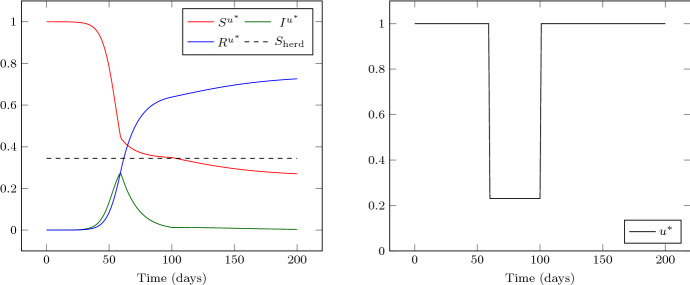
We first show in Figs. 3 and 4 the optimal solutions corresponding to the parameter choices $\alpha =0$ and ${\alpha }_{\mathrm{lock}}$, with $T=100$. To capture the full behavior of the trajectories, the computation window is [0, 200]. As expected the solutions are bang-bang. One also observes that the optimal value $S_{\infty ,\alpha ,T}^{\ast }$ is larger for smaller $\alpha$, as predicted in Theorem 2.2.

Fig. 3.

Solution of Problem ${\mathcal{P}}_{\alpha ,T}$ for $\alpha =0.0$ and $T=100$, displayed on the time interval [0, 200]. In this case $S_{\infty }^{\ast }=0.282$ and $T_0^{\ast }=61.9$

Fig. 4.

Solution of Problem ${\mathcal{P}}_{\alpha ,T}$ for $\alpha ={\alpha }_{\text{lock}}$ and $T=100$ displayed on the time interval [0, 200]. In this case $S_{\infty }^{\ast }=0.259$ and $T_0^{\ast }=59.2$

By using Lemma 4.2, it is easy to determine numerically the optimal value $S_{\infty ,\alpha ,T}^{\ast }$ by solving the equation

$$\begin{array}{c}\hfill S_{\infty ,\alpha ,T}^{\ast }-\frac{\gamma }{\beta }ln{S}_{\infty ,\alpha ,T}^{\ast }=S^{u^{\ast }}(T)+I^{u^{\ast }}(T)-\frac{\gamma }{\beta }ln{S}^{u^{\ast }}(T),\end{array}$$

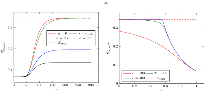
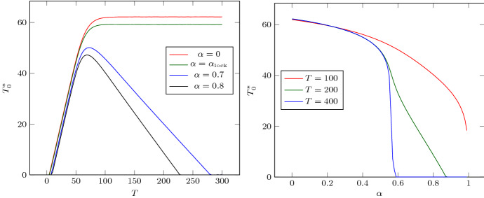
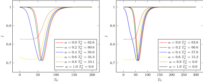
for $u^{\ast }$ solution of ${\mathcal{P}}_{\alpha ,T}$. This allows to investigate numerically in Figs. 5 and 6 the dependency of $S_{\infty ,\alpha ,T}^{\ast }$ and $T_0^{\ast }$ with respect to the parameters T and $\alpha$. As announced in Theorem 2.2, the optimal value $S_{\infty ,\alpha ,T}^{\ast }$ is nonincreasing with respect to $\alpha$ and nondecreasing with respect to T.

Fig. 5.

Graph of $S_{\infty ,\alpha ,T}^{\ast }$ for Problem ${\mathcal{P}}_{\alpha ,T}$ with respect to T for $\alpha \in \{0,{\alpha }_{\text{lock}},0.7,0.8\}$ (left) and with respect to $\alpha$ for $T\in \{100,200,400\}$ (right)

Fig. 6.

Graph of $T_0^{\ast }$ for Problem ${\mathcal{P}}_{\alpha ,T}$ with respect to T for $\alpha \in \{0.0,{\alpha }_{\text{lock}},0.7,0.8\}$ (left) and with respect to $\alpha$ for $T\in \{100,200,400\}$ (right)

In Fig. 5, for $T=400$, we observe numerically that the lower bound $\overline{\alpha }$ given in Theorem 2.1 and below which S can get as close as we want to $S_{\mathrm{herd}}$ over an infinite horizon, is optimal ($\overline{\alpha }\approx 0.56$). In particular, for lockdown conditions similar to the ones in effect in France between March and May 2020 ($\alpha \approx 0.231$), it appears that it is possible to come as close as desired to the optimal bound $S_{\mathrm{herd}}$ of inequality (4). Interestingly, we observe in Fig. 6-left that when $\alpha$ is too large, then $T_0=0$ for T large enough.

Another interesting feature can be observed in Fig. 6: the instant $T_0^{\ast }$ at which the optimal lockdown begins is almost independent of the level of the maximal lockdown $\alpha \in [0,0.8]$ for “small enough” duration T (say $T\le 60$ days). In other words, the optimal choice of this instant, and thus the optimal control itself, is robust with respect to the uncertainties on the lockdown duration and intensity, provided the former is not too long and the latter not too weak.

We also mention that Fig. 5-left gives the solution to the minimal time problem. Indeed, from Theorem 2.4, a control $u^{\ast }$ is optimal for ${\mathcal{P}}_{\alpha ,T}$ iff it is optimal for the minimal time problem. Then, given $\epsilon >0$ and $\alpha ⩽\overline{\alpha }$, the minimal time of action such that the final value of susceptible is at a distance $\epsilon$ of $S_{\mathrm{herd}}$ is obtained by computing the intersection of the curves in Fig. 5-left with the horizontal line $S_{\mathrm{herd}}-\epsilon$. As expected, when $\alpha$ is too large, i.e., when the lockdown is insufficient, the solution stays far away from $S_{\mathrm{herd}}$ (see Fig. 5-right).

We conclude this section by examining in Fig. 7 the influence of the initial data, $S_0$ and $I_0$, on the optimal intervention time. Let us mention that, in agreement with the conclusions of [15], the numerical simulation in this figure seems to indicate that the larger the quantity $I_0$, the earlier the optimal lockdown strategy should be applied.

Fig. 7.

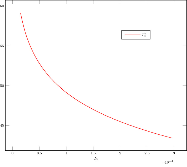
Numerical simulation of the SIR model with the numerical parameters $\beta$, $\gamma$, ${\alpha }_{\mathrm{lock}}$ and $R_0$ given in Table 2. The optimal time $T_0^{\ast }$ introduced in Theorem 2.3 is plotted with respect to $I_0\in [1.49\times {10}^{-5},2.95\times {10}^{-4}]$ (corresponding to an initial number of infected people between $1\times {10}^3$ and $2\times {10}^4$ for a total number of people of $6.7\times {10}^7$) and $S_0$ is chosen so that $S_0+I_0=6.7\times {10}^7$

Proofs of the Main Results

Preliminary Results

Before proving the main results, we provide some useful elementary properties of the state variables (S, I) solving (5) whose role in the sequel will be central. To this aim, it is convenient to introduce the function ${\Phi }_{\xi }$ defined for any $\xi >0$

$$\begin{array}{c}\hfill {\Phi }_{\xi }:{\mathbb{R}}_{+}^{\ast }\times {\mathbb{R}}_{+}\ni (S,I)⟼S+I-\frac{1}{\xi }lnS.\end{array}$$ 10

Let us start with a preliminary result regarding the values of ${\Phi }_{\xi }$ along the trajectories of System (5).

Lemma 4.1

For any $u\in L^{\infty }([0,+\infty ),[0,1])$ and $\xi \in \mathbb{R}$, one has

$$\begin{array}{c}\hfill \frac{d}{\mathit{dt}}\left[{\Phi }_{\xi },(S(t),I(t))\right]=\left(\frac{\beta }{\xi },u,(t),-,\gamma \right)I\end{array}$$ 11

along any trajectory of system (5). In particular, if u is constant on a nonempty, possibly unbounded, interval, then the function ${\Phi }_{{\mathcal{R}}_{0}u}(S(·),I(·))$ is constant on this interval along any trajectory of System (5).

Proof

The proof of (11) follows from straightforward computations. Indeed along every trajectory of (5), one has

$$\begin{array}{c}\hfill \frac{\mathrm{d}}{\mathrm{d}t}\left[{\Phi }_{\xi },(S(t),I(t))\right]=\frac{\mathrm{d}}{\mathrm{d}t}\left(S,+,I,-,\frac{1}{\xi },ln,S\right)=\left(1,-,\frac{1}{\xi S}\right)\dot{S}+\dot{I}=\left(\frac{\beta }{\xi },u,(t),-,\gamma \right)I.\end{array}$$

The second part of the statement is an obvious byproduct of this property, by setting $\xi ={\mathcal{R}}_{0}u$. $\square$

Lemma 4.1 allows to characterize the value of the limit of S at infinity, as now stated.

Lemma 4.2

Let $u\in {\mathcal{U}}_{\alpha ,T}$. For any trajectory of (5), the limit $S_{\infty }(u)$ of S(t) at infinity exists and is the unique solution in the interval $[0,1/{\mathcal{R}}_0]$ of the equation

$$\begin{array}{c}\hfill {\Phi }_{{\mathcal{R}}_0}\left(S_{\infty },,,0\right)={\Phi }_{{\mathcal{R}}_0}\left(S,(,T,),,,I,(,T,)\right),\end{array}$$ 12

where ${\Phi }_{{\mathcal{R}}_0}$ is given by (10).

Proof

Any input control u from ${\mathcal{U}}_{\alpha ,T}$ is equal to 1 on $[T,+\infty )$. Hence, applying Lemma 4.1 with $u=1$ on this interval yields (12), by continuity of ${\Phi }_{{\mathcal{R}}_0}$ and because of (2). Moreover, Eq. (12) has exactly two roots. Indeed, this follows by observing that the mapping $S\mapsto {\Phi }_{{\mathcal{R}}_0}(S,0)$ is first decreasing and then increasing on $(0,+\infty )$, with infinite limit at $0^{+}$ and $+\infty$, and minimal value at $S=1/{\mathcal{R}}_0=S_{\mathrm{herd}}$, equal to $\frac{1}{{\mathcal{R}}_0}(1+ln{\mathcal{R}}_0)$. We conclude by noting that the limit $S_{\infty }(u)$ cannot be larger than $S_{\mathrm{herd}}$: otherwise there would exist $\epsilon >0$ such that $\dot{I}>\epsilon >0$ and $\dot{S}<-\epsilon \beta S$ for T large enough, so that S would tend to zero at infinity, yielding a contradiction. It follows that the value of $S_{\infty }(u)$ is thus the smallest root of (12).

Remark 4.1

(On the control in infinite time) Notice that, in the quite unrealistic situation where one is able to act on System (5) up to an infinite horizon of time, then the optimal strategy to maximize $S_{\infty }(u)$ is to consider the constant control function $u_{\alpha }(·)=\alpha$ on $[0,+\infty )$. Indeed, according to Lemma 4.1,

$$\begin{array}{c}\hfill \frac{\mathrm{d}}{\mathrm{d}t}\left[{\Phi }_{\alpha {\mathcal{R}}_0},(S(t),I(t))\right]=\left(\frac{\beta }{\alpha {\mathcal{R}}_0},u,(t),-,\gamma \right)I(t)=\frac{\gamma }{\alpha }(u(t)-\alpha )I(t)⩾0,\end{array}$$

for all $t\in [0,T]$. Hence, ${\Phi }_{\alpha {\mathcal{R}}_0}(S_0,I_0)⩽{\Phi }_{\alpha {\mathcal{R}}_0}(S_{\infty }(u),0),$ with equality if, and only if $u=u_{\alpha }=\alpha$ a.e. on ${\mathbb{R}}_{+}$. Since $S_{\infty }(u)$ is maximal whenever ${\Phi }_{\alpha {\mathcal{R}}_0}(S_{\infty }(u),0)$ is minimal, we get that the optimal strategy in that case corresponds to the choice $u=u_{\alpha }=\alpha$ a.e. on ${\mathbb{R}}_{+}$. Moreover, it is notable that this maximal value $S_{\infty }(u_{\alpha })$ is computed by solving the nonlinear equation ${\Phi }_{\alpha {\mathcal{R}}_0}(S_{\infty },0)={\Phi }_{\alpha {\mathcal{R}}_0}(S_0,I_0)$. Therefore, an easy application of the implicit functions theorem yields that the mapping $\alpha \mapsto S_{\infty }(u_{\alpha })$ is decreasing.

Proof of Theorem 2.1

Let us start with (i). According to (5), one has $\dot{I}⩾-\gamma I$, thus $I(t)⩾I_0{e}^{-\gamma t}>0$ for all $t>0$. Then, $\dot{S}<0$ and S is decreasing. Assume by contradiction that, for all $t>0$, we have $S_{\mathrm{herd}}⩽S(t)$. Since I satisfies (5), it follows that $\dot{I}⩾0$ on $(T,+\infty )$ and then, $\dot{S}⩽-\beta I(T)S$ on $(T,+\infty )$. We thus infer that $S(t)⩽e^{-\beta I(T)(t-T)}S(T)$ for $t>T$, and thus $S(t)\to 0$ as $t\to +\infty$, which is a contradiction.

Let us now show (ii). For all $\alpha \in [0,1)$, we denote by $u_{\alpha }(·)$ the control equal to $\alpha$ on $(0,\infty )$. Thanks to the same argument by contradiction as above, one has $S_{\infty }(u_{\overline{\alpha }})⩽1/(\overline{\alpha }{\mathcal{R}}_0)$. Let us denote by $(S^{u_{\overline{\alpha }}},I^{u_{\overline{\alpha }}})$ the solution to System (5) associated to $u_{\overline{\alpha }}$. Lemma 4.1 shows that the function $t\mapsto {\Phi }_{\overline{\alpha }{\mathcal{R}}_0}(S^{u_{\overline{\alpha }}}(t),I^{u_{\overline{\alpha }}}(t))$ is conserved, and we infer that $S_{\infty }(u_{\overline{\alpha }})$ solves the equation

$$\begin{array}{c}\hfill {\Phi }_{\overline{\alpha }{\mathcal{R}}_0}\left(S_0,,,I_0\right)={\Phi }_{\overline{\alpha }{\mathcal{R}}_0}\left(S_{\infty },\left(u_{\overline{\alpha }}\right),,,0\right).\end{array}$$

Using the expression of $\overline{\alpha }$,

$$\begin{array}{c}\hfill {\Phi }_{\overline{\alpha }{\mathcal{R}}_0}\left(S_{\mathrm{herd}},,,0\right)={\Phi }_{\overline{\alpha }{\mathcal{R}}_0}\left(S_0,,,I_0\right)={\Phi }_{\overline{\alpha }{\mathcal{R}}_0}\left(S_{\infty },\left(u_{\overline{\alpha }}\right),,,0\right).\end{array}$$

Since $x\mapsto {\Phi }_{\overline{\alpha }{\mathcal{R}}_0}(x,0)$ is bijective on $(0,\frac{1}{\overline{\alpha }{\mathcal{R}}_0})$, we deduce that $S_{\infty }(u_{\overline{\alpha }})=S_{\mathrm{herd}}$. It follows that for $\eta >0$ small enough, there exists $T>0$ such that for each $t>T$, ${\dot{I}}^{u_{\overline{\alpha }}}(t)⩽(\beta \overline{\alpha }(1+\eta )\frac{\gamma }{\beta }-\gamma )I^{u_{\overline{\alpha }}}(t)<0$. By using a Gronwall lemma, one infers that $I^{u_{\overline{\alpha }}}(t)\to 0$ as $t\to +\infty$. Then, for all $k\in {\mathbb{N}}^{\ast }$, there exists $T_k>0$, such that $|S^{u_{\overline{\alpha }}}(T_k)-S_{\mathrm{herd}}|⩽1/k$ and $I^{u_{\overline{\alpha }}}(T_k)⩽1/k$. Consider $u_k:=\overline{\alpha }{\mathbb{1}}_{(0,T_k)}+{\mathbb{1}}_{(T_k,\infty )}$ and let us denote by $(S^{u_k},I^{u_k})$ the solution to System (5) associated to $u_k$. By continuity of ${\Phi }_{{\mathcal{R}}_0}$,

$$\begin{array}{c}\hfill {\Phi }_{{\mathcal{R}}_0}\left(S_{\infty },(u_k),,,0\right)={\Phi }_{{\mathcal{R}}_0}\left(S^{u_k},\left(T_k\right),,,I^{u_k},\left(T_k\right)\right)\underset{k\to \infty }{⟶}{\Phi }_{{\mathcal{R}}_0}\left(S_{\mathrm{herd}},,,0\right).\end{array}$$

Thus $S_{\infty }(u_k)\underset{k\to \infty }{⟶}{S}_{\mathrm{herd}}$.

Let us finally prove (iii). We show that $\alpha \mapsto S_{\infty }(u_{\alpha })$ is strictly decreasing. Let ${\alpha }_1,{\alpha }_2\in [0,1)$ such that ${\alpha }_1<{\alpha }_2$ and $(S^{u_{{\alpha }_1}},I^{u_{{\alpha }_1}})$ and $(S^{u_{{\alpha }_2}},I^{u_{{\alpha }_2}})$ the solutions to System (5) associated to $u_{{\alpha }_1}$ and $u_{{\alpha }_2}$, respectively. Using Lemma 4.1, $t\mapsto {\Phi }_{{\alpha }_1{\mathcal{R}}_0}(S^{u_{{\alpha }_2}}(t),I^{u_{{\alpha }_2}}(t))$ is strictly increasing, hence

$$\begin{array}{c}\hfill {\Phi }_{{\alpha }_1{\mathcal{R}}_0}\left(S_{\infty },(u_{{\alpha }_1}),,,0\right)={\Phi }_{{\alpha }_1{\mathcal{R}}_0}\left(S_0,,,I_0\right)<{\Phi }_{{\alpha }_1{\mathcal{R}}_0}\left(S_{\infty },\left(u_{{\alpha }_2}\right),,,0\right).\end{array}$$

Thanks to the equations satisfied by $(S^{u_{{\alpha }_1}},I^{u_{{\alpha }_1}})$ and $(S^{u_{{\alpha }_2}},I^{u_{{\alpha }_2}})$, one has $S_{\infty }(u_{{\alpha }_1})$, $S_{\infty }(u_{{\alpha }_2})⩽S_{\mathrm{herd}}/{\alpha }_1$. Since $x\mapsto {\Phi }_{{\alpha }_1{\mathcal{R}}_0}(x,0)$ in strictly decreasing on $(0,S_{\mathrm{herd}}/{\alpha }_1)$, we deduce that $S_{\infty }(u_{{\alpha }_2})<S_{\infty }(u_{{\alpha }_1})$. This concludes the proof since $S_{\infty }(u_{\overline{\alpha }})=S_{\mathrm{herd}}$.

Proof of Theorem 2.2

Solving ${\mathcal{P}}_{\alpha ,T}$ involves the resolution of an ODE system on an infinite horizon, and it is quite convenient to consider an equivalent version of this problem involving an ODE system on a bounded horizon. A key point for this is that, according to Lemma 4.2, $S_{\infty }$ solves Eq. (12). Furthermore, since the mapping $[0,1/{\mathcal{R}}_0]\ni S\mapsto {\Phi }_{{\mathcal{R}}_0}(S,0)$ is decreasing, maximizing $S_{\infty }$ is equivalent to minimize ${\Phi }_{{\mathcal{R}}_0}(S_{\infty },0)$. Combining all these observations yields that the optimal control problem is equivalent to the following problem, investigated hereafter: where

$$\begin{array}{c}\hfill J(u):={\Phi }_{{\mathcal{R}}_0}(S(T),I(T))\end{array}$$ 13

and (S, I) solves the controlled system (5) associated to the control $u(·)$.

Proof of Theorem 2.2

For better readability, the proof of Theorem 2.2 is decomposed into several steps.

Step 1: existence of an optimal control We will prove the existence of an optimal control for the equivalent problem ${\mathcal{P}}_{\alpha ,T}^{\Phi }$. Let ${(u_n)}_{n\in \mathbb{N}}$ be a maximizing sequence for Problem ${\mathcal{P}}_{\alpha ,T}^{\Phi }$. Since ${(u_n)}_{n\in \mathbb{N}}$ is uniformly bounded, we may extract a subsequence still denoted ${(u_n)}_{n\in \mathbb{N}}$ with a slight abuse of notation, converging toward $u^{\ast }$ for the weak-star topology of $L^{\infty }(0,T)$. It is moreover standard that ${\mathcal{U}}_{\alpha ,T}$ is closed for this topology and therefore, $u^{\ast }$ belongs to ${\mathcal{U}}_{\alpha ,T}$. For $n\in \mathbb{N}$, let us denote $(S_n,I_n)$ the solution to the SIR model (5) associated to $u=u_n$. A straightforward application of the Cauchy–Lipschitz theorem yields that ${({\dot{S}}_n,{\dot{I}}_n)}_{n\in \mathbb{N}}$ is uniformly bounded. By applying Ascoli’s theorem, we may extract a subsequence still denoted ${(S_n,I_n)}_n$ that converges toward $(S^{\ast },I^{\ast })$ in $C^0([0,T])$. As usually, we consider an equivalent formulation of System (5), where $(S_n,I_n)$ can be seen as the unique fixed point of an integral operator. We then pass to the limit and show that $(S^{\ast },I^{\ast })$ solves the same equation where u has been replaced by $u^{\ast }$. By combining all these facts with the continuity of ${\Phi }_{{\mathcal{R}}_0}$, we then infer that ${(J(u_n))}_{n\in \mathbb{N}}$ converges up to a subsequence to $J(u^{\ast })$, which gives the existence.

Step 2: optimality conditions and bang-bang property We will again establish these properties for the equivalent problem ${\mathcal{P}}_{\alpha ,T}^{\Phi }$. In what follows, for the sake of simplicity, we will consider and denote by u a solution to Problem ${\mathcal{P}}_{\alpha ,T}^{\Phi }$ and by (S, I), the associated pair solving System (5). Observe first that integrating (11) in Lemma 4.1, one has

$$\begin{array}{c}\hfill J(u)={\Phi }_{{\mathcal{R}}_0}(S(T),I(T))={\Phi }_{{\mathcal{R}}_0}(S_0,I_0)+\gamma {\int }_0^T(u(t)-1)I(t)dt.\end{array}$$

It is standard to write the first-order optimality conditions for such kind of optimal control problem. To this aim, we use the so-called Pontryagin maximum principle (see, e.g., [31]) and introduce the Hamiltonian $\mathcal{H}$ defined on ${\mathbb{R}}^4$ by

$$\begin{array}{cc}\hfill \mathcal{H}(S,I,p_S,p_I)=& \left[-,p_S,\beta ,u,S,+,p_I,(\beta uS-\gamma ),-,\gamma ,(u-1)\right]I\hfill \\ \hfill =& \gamma (1-p_I)I+\left(\beta ,\left(p_I,-,p_S\right),S,-,\gamma \right)Iu.\hfill \end{array}$$

There exists an absolutely continuous mapping $(p_S,p_I):[0,T]\to {\mathbb{R}}^2$ called adjoint vector such that the extremal $((S,I),(p_S,p_I),u)$ satisfies a.e. in [0, T]:

Adjoint equations and transversality conditions:

$$\begin{array}{cc}\hfill {\dot{p}}_S=& \beta uI\left(p_S,-,p_I\right),{\dot{p}}_I=\beta uS{p}_S-\left(\beta ,u,S,-,\gamma \right)p_I+\gamma (u-1),\hfill \end{array}$$ 14a

$$\begin{array}{cc}\hfill p_S(T)=& 0,p_I(T)=0.\hfill \end{array}$$ 14b

Maximization condition: for a.e. $t\in [0,T]$, u(t) solves the problem

$$\begin{array}{c}\hfill \underset{\alpha ⩽v⩽1}{max}\left(\beta ,\left(p_I,(t),-,p_S,(t)\right),S,(t),-,\gamma \right)I(t)v\end{array}$$

and therefore, by using that I is nonnegative on [0, T], one has

$$\begin{array}{c}\hfill w⩾-\frac{1}{{\mathcal{R}}_0}\text{on}\{u=\alpha \},w⩽-\frac{1}{{\mathcal{R}}_0}\text{on}\{u=1\},w=-\frac{1}{{\mathcal{R}}_0}\text{on}\{\alpha <u<1\},\end{array}$$ 15

where w denotes the Lipschitz-continuous switching function given by $w=S(p_S-p_I)$.

By using (5), one computes

$$\begin{array}{cc}\hfill \dot{w}=& -\beta uSI\left(p_S,-,p_I\right)+S\left(-,\beta ,u,I,\left(p_I,-,p_S\right)\right)\hfill \\ \hfill & \left(+,\beta ,u,S,\left(p_I,-,p_S\right),-,\gamma ,p_I,-,\gamma ,(u-1)\right)\hfill \\ \hfill =& -S\left(\beta ,u,w,+,\gamma ,(,p_I,+,u,-,1,)\right).\hfill \end{array}$$

We will now prove that the optimal control can be written as $u_{T_0}$ defined in (7), for some $T_0\in [0,T)$. From (14b), one has $p_S(T)=p_I(T)=0$, and thus $w(T)=0>-\frac{1}{{\mathcal{R}}_0}$. According to (15) and by continuity of w, this implies $u(·)=\alpha$ on a certain maximal interval $[T_0,T]$, for some $T_0\in (0,T)$, by continuity of w. By inserting the relation $w⩾-\frac{1}{{\mathcal{R}}_0}$ holding on $(T_0,T)$ in Eq. (14a) satisfied by $p_I$, we deduce that ${\dot{p}}_I⩾\gamma (p_I-1)$ on $(T_0,T)$. Since $p_I(T)=0$, the Gronwall lemma yields

$$\begin{array}{c}\hfill p_I(t)⩽1-e^{\gamma (t-T)},t\in [T_0,T].\end{array}$$ 16

Then, either $T_0=0$, in which case, $u=u_0=\alpha {\mathbb{1}}_{[0,T]}+{\mathbb{1}}_{[T,+\infty )}$ (see (7)) or $T_0>0$. Let us now address this latter case. Since the interval $(T_0,T)$ is maximal by assumption and w is continuous, one has necessarily $w(T_0)=-1/{\mathcal{R}}_0$. On the other hand, S and $p_I$ are continuous, with $p_I(T_0)<1$ according to (16). Consequently, for any $\epsilon$ in the nonempty open interval $(0,\gamma S(T_0)(1-p_I(T_0))$, there exists a neighborhood ${\mathcal{V}}_{T_0}$ of $T_0$ on which

$$\begin{array}{cc}\hfill \dot{w}=& -\beta uS\left(w,+,\frac{1}{{\mathcal{R}}_0}\right)+\gamma S\left(1,-,p_I\right)\hfill \\ \hfill \in & \left[\gamma ,S,\left(T_0\right),\left(1,-,p_I,\left(T_0\right)\right),-,\epsilon ,,,\gamma ,S,\left(T_0\right),\left(1,-,p_I,\left(T_0\right)\right),+,\epsilon \right]\text{a.e.}\hfill \end{array}$$

Since $\epsilon \in (0,\gamma S(T_0)(1-p_I(T_0))$, this implies that w is strictly increasing in ${\mathcal{V}}_{T_0}$. Therefore, there exists a maximal open interval $(T_1,T_0)$ with $T_1\in [0,T_0)$ on which $w<-\frac{1}{{\mathcal{R}}_0}$, and therefore on which $u=1$. As a consequence, the left derivative of w at $T_0$ exists and reads

$$\begin{array}{c}\hfill \dot{w}\left(T_0^{-}\right)=-\beta S\left(T_0\right)\left(w,\left(T_0\right),+,\frac{1}{{\mathcal{R}}_0},p_I,\left(T_0\right)\right)>0.\end{array}$$ 17

We will in fact show that $T_1=0$. In other words, the control u can be written as (7).

To this aim, let us assume by contradiction that there exists $T_1\in (0,T_0)$ such that $w(T_1)=-\frac{1}{{\mathcal{R}}_0}=w(T_0)$ and $w<-\frac{1}{{\mathcal{R}}_0}$ on $(T_1,T_0)$. Observing that w is differentiable on $(T_1,T_0)$ and using Rolle’s theorem yields the existence of $\tau \in (T_1,T_0)$ such that $\dot{w}(\tau )=0$.

Note that, according to (14a), one has $\dot{w}=-S{\dot{p}}_I$, a.e. in (0, T). Since $S(\tau )>0$, one has also ${\dot{p}}_I(\tau )=0$. Using the fact that $u=1$ on $(T_1,T_0)$, this means that the point $(p_I(\tau ),w(\tau ))$ is a steady-state of the system

$$\begin{array}{c}\hfill \dot{w}=-\beta Sw-\gamma S{p}_I,{\dot{p}}_I=\beta w+\gamma p_I.\end{array}$$

According to the Cauchy–Lipschitz theorem, we infer that $(p_I,w)$ is constant on $[\tau ,T_0]$ and therefore, ${\dot{p}}_I(T_0^{-})=\dot{w}(T_0^{-})=0$, which is in contradiction with (17). As a conclusion, $T_1=0$, and u can be written as (7).

Step 3: monotonicity of $S_{\infty ,\alpha ,T}^{\ast }$ Let $T>0$ and $0⩽\alpha ⩽\tilde{\alpha }<1$. It is straightforward that ${\mathcal{U}}_{\tilde{\alpha },T}\subset {\mathcal{U}}_{\alpha ,T}$, and then $S_{\infty ,\alpha ,T}^{\ast }⩾S_{\infty ,\tilde{\alpha },T}^{\ast }$. It follows that the map $[0,1)\ni \alpha \mapsto {max}_{u\in {\mathcal{U}}_{\alpha ,T}}{S}_{\infty }(u)$ is nonincreasing.

Let us show that the map $T\mapsto {max}_{u\in {\mathcal{U}}_{\alpha ,T}}{S}_{\infty }(u)$ is nondecreasing. Let $0<T⩽\tilde{T}$, $0⩽\alpha <1$, and denote by $u^{\ast }\in {\mathcal{U}}_{\alpha ,T}$ the control realizing the maximum $S_{\infty ,\alpha ,T}^{\ast }$. Since $u^{\ast }=1$ in $(T,\tilde{T})$, one has $u^{\ast }\in {\mathcal{U}}_{\alpha ,\tilde{T}}$. Thus

$$\begin{array}{c}\hfill S_{\infty ,\alpha ,\tilde{T}}^{\ast }⩾S_{\infty }\left(u^{\ast }\right)=S_{\infty ,\alpha ,T}^{\ast }.\end{array}$$

Step 4: uniqueness of the optimal control The demonstration of the uniqueness of the optimal control is achieved in the proof of Theorem 2.3 below, by demonstrating the uniqueness of the optimal switching point $T_0$. Except this point, the demonstration of Theorem 2.2 is now complete. $\square$

Proof of Theorem 2.3

The proof is decomposed into several steps. We assume first that $\alpha >0$, the case $\alpha =0$ is considered in the last step. In the whole proof, one deals with control functions $u_{T_0}$ as defined in formula (7).

Step 1: necessary first order optimality conditions on $T_0$ Let $u=u_{T_0}$ be an optimal control for problem ${\mathcal{P}}_{\alpha ,T}$, with $T_0$ be the associated optimal switching time. Let us introduce the criterion j given by

$$\begin{array}{c}\hfill j\left(T_0\right):={\Phi }_{{\mathcal{R}}_0}\left(S^{T_0},(T),,,I^{T_0},(T)\right)=I^{T_0}(T)+S^{T_0}(T)-\frac{\gamma }{\beta }ln{S}^{T_0}(T),\end{array}$$ 18

where $(S^{T_0},I^{T_0})$ is the solution corresponding to the control $u_{T_0}$, as previously defined. For the sake of simplicity, we omit these subscripts in the sequel. By Theorem 2.2, it is equivalent to minimize J defined in (13) and to minimize j. By using Lemma 4.2, one has

$$\begin{array}{c}\hfill \begin{array}{cc}I(t)+S(t)-\frac{\gamma }{\beta }lnS(t)=c_0\hfill & \text{in}\left[0,,,T_0\right],\hfill \\ I(t)+S(t)-\frac{\gamma }{\alpha \beta }lnS(t)=I\left(T_0\right)+S\left(T_0\right)-\frac{\gamma }{\alpha \beta }lnS\left(T_0\right)\hfill & \text{in}\left[T_0,,,T\right],\hfill \end{array}\end{array}$$ 19

where $c_0=I_0+S_0-\frac{\gamma }{\beta }ln{S}_0$. According to (19), we infer that S solves the system

$$\begin{array}{cc}\hfill \dot{S}& =-\beta S(c_0-S+\frac{\gamma }{\beta }lnS),\text{in}(0,T_0),\hfill \end{array}$$ 20a

$$\begin{array}{cc}\hfill \dot{S}& =-\alpha \beta S\left(c_0,+,\frac{\gamma }{\beta },\left(1,-,\frac{1}{\alpha }\right),ln,S,\left(T_0\right),-,S,+,\frac{\gamma }{\alpha \beta },ln,S\right),\text{in}\left(T_0,,,T\right),\hfill \end{array}$$ 20b

with the initial data $S(0)=S_0$. Using (19), one gets

$$\begin{array}{cc}\hfill j\left(T_0\right)=& I(T)+S(T)-\frac{\gamma }{\beta }lnS(T)\hfill \\ \hfill =& I\left(T_0\right)+S\left(T_0\right)-\frac{\gamma }{\alpha \beta }lnS\left(T_0\right)+\frac{\gamma }{\beta }\left(\frac{1}{\alpha },-,1\right)lnS(T)\hfill \\ \hfill =& c_0+\frac{\gamma }{\beta }lnS\left(T_0\right)-\frac{\gamma }{\alpha \beta }lnS\left(T_0\right)+\frac{\gamma }{\beta }\left(\frac{1}{\alpha },-,1\right)lnS(T),\hfill \end{array}$$

so that the cost function reads

$$\begin{array}{c}\hfill j\left(T_0\right)=c_0+\frac{\gamma }{\beta }\left(\frac{1}{\alpha },-,1\right)ln\left(\frac{S(T)}{S\left(T_0\right)}\right).\end{array}$$

The next lemma allows to compute the derivative of j with respect to $T_0$. For the sake of clarity, its proof is postponed to the end of this section.

Lemma 4.3

For all $t\in [T_0,T]$, the derivative3$\widehat{S}(t)$ and $\widehat{S(T_0)}$ of the function $S(·)$ and $S(T_0)$ with respect to $T_0$, in other words $\widehat{S}(t)=\frac{\partial S(t)}{\partial T_0}$ and $\widehat{S(T_0)}=\frac{\partial [S(T_0)]}{\partial T_0}$, are given by

$$\begin{array}{c}\hfill \widehat{S}(t)=(\alpha -1)\beta S(t)I(t)\left(1,+,\gamma ,I,\left(T_0\right),{\int }_{T_0}^t,\frac{\mathit{ds}}{I(s)}\right)\end{array}$$

and

$$\begin{array}{c}\hfill \widehat{S\left(T_0\right)}=-\beta S\left(T_0\right)I\left(T_0\right).\end{array}$$

Thanks to this result, we may compute

$$\begin{array}{cc}\hfill j^{\prime }\left(T_0\right)=& \frac{\gamma }{\beta }\left(\frac{1}{\alpha },-,1\right)\left(\frac{\widehat{S}(T)}{S(T)},-,\frac{\widehat{S\left(T_0\right)}}{S\left(T_0\right)}\right)\hfill \\ \hfill =& \gamma \left(\frac{1}{\alpha },-,1\right)\left((\alpha -1),I,(T),\left(1,+,\gamma ,I,\left(T_0\right),{\int }_{T_0}^T,\frac{\mathit{ds}}{I(s)}\right),+,I,\left(T_0\right)\right)\hfill \\ \hfill =& \gamma \left(\frac{1}{\alpha },-,1\right)I\left(T_0\right)(\alpha -1)\left(\frac{I(T)}{I\left(T_0\right)},+,\gamma ,{\int }_{T_0}^T,\frac{I(T)}{I(s)},d,s,-,\frac{1}{1-\alpha }\right).\hfill \end{array}$$

By noting that

$$\begin{array}{c}\hfill {\int }_{T_0}^T\frac{S(t)}{I(t)}dt=\&\frac{1}{\alpha \beta }{\int }_{T_0}^T\frac{\alpha \beta S(t)-\gamma +\gamma }{I(t)}dt=\frac{1}{\alpha \beta }{\int }_{T_0}^T\frac{\dot{I}(t)}{I{(t)}^2}dt+\frac{\gamma }{\alpha \beta }{\int }_{T_0}^T\frac{1}{I(t)}dt\\ \hfill =\&\frac{1}{\alpha \beta }\left(\frac{1}{I\left(T_0\right)},-,\frac{1}{I(T)},+,\gamma ,{\int }_{T_0}^T,\frac{1}{I(t)},,d,t\right),\end{array}$$

we have for the function $\psi$ defined in (8):

$$\begin{array}{c}\hfill \psi \left(T_0\right)=\left(\frac{1}{\alpha },-,1\right)\left(\frac{I(T)}{I\left(T_0\right)},+,\gamma ,{\int }_{T_0}^T,\frac{I(T)ds}{I(s)},-,\frac{1}{1-\alpha }\right).\end{array}$$ 21

We deduce that $j^{\prime }(T_0)=0$ is equivalent to

$$\begin{array}{c}\hfill \psi \left(T_0\right)=0.\end{array}$$ 22

Step 2: Zeros of $j^{\prime }$ and uniqueness of the optimal switching time According to (5), one has for any $t\in (T_0,T)$, $I(t)=I(T_0)exp\left({\int }_{T_0}^t,(\alpha \beta S(s)-\gamma ),,d,s\right)$. Then, using the expression of $\psi$ given in (21), it follows that

$$\begin{array}{c}\hfill \psi \left(T_0\right)=\&\left(\frac{1}{\alpha },-,1\right)exp\left({\int }_{T_0}^T,\left(\alpha ,\beta ,S,(,s,),-,\gamma \right),,d,s\right)\\ \hfill & +(\frac{1}{\alpha }-1)\gamma {\int }_{T_0}^{T}exp\left({\int }_t^T,\left(\alpha ,\beta ,S,(,s,),-,\gamma \right),,d,s\right)dt-\frac{1}{\alpha }.\hfill \end{array}$$

Introducing $\phi :[0,T]\to \mathbb{R}$ defined by $\phi (t)=exp\left({\int }_t^T,(\alpha \beta S(s)-\gamma ),,d,s\right)$, the last expression writes simply

$$\begin{array}{c}\hfill \psi \left(T_0\right)=\left(\frac{1}{\alpha },-,1\right)\phi \left(T_0\right)+\left(\frac{1}{\alpha },-,1\right)\gamma {\int }_{T_0}^T\phi (t)dt-\frac{1}{\alpha }.\end{array}$$

Differentiating this identity with respect to $T_0$ yields

$$\begin{array}{cc}\hfill {\psi }^{\prime }\left(T_0\right)=& \left(\frac{1}{\alpha },-,1\right)\left(-,\alpha ,\beta ,S,\left(T_0\right),+,\gamma ,+,{\int }_{T_0}^T,\alpha ,\beta ,\widehat{S},(s),,d,s\right)\phi \left(T_0\right)\hfill \\ \hfill & -\gamma \left(\frac{1}{\alpha },-,1\right)\phi \left(T_0\right)+\gamma (\frac{1}{\alpha }-1){\int }_{T_0}^T\left({\int }_t^T,\alpha ,\beta ,\widehat{S},(s),,d,s\right)\phi (t)dt\hfill \\ \hfill =& \left(\frac{1}{\alpha },-,1\right)\left(-,\alpha ,\beta ,S,\left(T_0\right),+,{\int }_{T_0}^T,\alpha ,\beta ,\widehat{S},(s),,d,s\right)\phi \left(T_0\right)\hfill \\ \hfill & +\gamma \left(\frac{1}{\alpha },-,1\right){\int }_{T_0}^T\left({\int }_t^T,\alpha ,\beta ,\widehat{S},(s),,d,s\right)\phi (t)dt.\hfill \end{array}$$

As a consequence of Lemma 4.3, both terms in the previous formula are negative, and ${\psi }^{\prime }(T_0)<0$. The function $\psi$ is thus decreasing on (0, T). Moreover, $\psi (T)=-1<0$. Therefore, if $\psi (0)<0$, then (22), or equivalently $j^{\prime }(T_0)=0$, has no solution, and thus $T_0^{\ast }=0$. Conversely, if $\psi (0)\ge 0$, then (22) admits a unique solution $T_0^{\ast }$ which is the unique critical point of j. In particular, in the case $\psi (0)=0$, one has $T_0^{\ast }=0$.

We also deduce that the function j is nonincreasing on $(0,T_0^{\ast })$ and increasing on $(T_0^{\ast },T)$.

Step 3: $S(0)⩽S_{\mathrm{herd}}$ implies $T_0^{\ast }=0$ We consider now the particular case where $S(0)⩽S_{\mathrm{herd}}$, and show that in this case $T_0^{\ast }=0$. As S is decreasing, one then has $S(t)⩽S_{\mathrm{herd}}$ for any $t⩾0$, whatever the input control. Thus, for any $t\in [0,T]$, one has $\phi (t)⩽{\int }_t^T(\alpha \beta S_{\mathrm{herd}}-\gamma )ds=\gamma (\alpha -1)(T-t)⩽0$, and

$$\begin{array}{c}\hfill \psi (0)=\left(\frac{1}{\alpha },-,1\right)\phi (0)+\left(\frac{1}{\alpha },-,1\right)\gamma {\int }_0^T\phi (t)dt-\frac{1}{\alpha }\end{array}$$

appears as a sum of three nonpositive terms. Therefore, $\psi (0)⩽0$, and we conclude that $T_0^{\ast }=0$ if $S(0)⩽S_{\mathrm{herd}}$.

Step 4: $T_0^{\ast }>0$ implies $S(T_0^{\ast })⩾S_{\mathrm{herd}}$, that is $T_0^{\ast }⩽{(S)}^{-1}(S_{\mathrm{herd}})$ To prove this estimate on $T_0^{\ast }$, consider an optimal trajectory for which the switching point verifies $T_0^{\ast }>0$ and $S(T_0^{\ast })<S_{\mathrm{herd}}$. By continuity, there exists a time instant $T_1\in (0,T_0^{\ast })$ such that $S(T_0^{\ast })<S(T_1)<S_{\mathrm{herd}}$. The point $(S(T_1),I(T_1))$ pertains to the optimal trajectory of the initial optimal control problem.

Consider now the optimal control problem defined by the same cost function, but with initial condition $(S(T_1),I(T_1))$ and on a time horizon of length $T-T_1$. The cost that is considered is the supremum of the limits of S among every admissible control inputs, so the optimal value for the second problem (on horizon $T-T_1$) is equal to the optimal value for the initial problem (on horizon T); and the optimal control for the former problem is indeed the restriction to $[T_1,T]$ of the optimal control for the latter problem. As a matter of case, if this was not the case, then concatenating the restriction to $[0,T_1]$ of the optimal solution of the problem on horizon T, with the optimal solution of the problem on horizon $T-T_1$, would lead to a larger limit of S at infinity.

Now observe that the optimal solution of the problem on $[0,T-T_1]$ takes on the value 1 on $[0,T_0^{\ast }-T_1]$, and then $\alpha$ on $[T_0^{\ast }-T_1,T-T_1]$. Therefore, it presents a commutation at time $T_0^{\ast }-T_1>0$, while the initial state value $(S(T_1),I(T_1))$ fulfills $S(T_1)<S_{\mathrm{herd}}$. But it was shown in Step 3 that such a situation is impossible. As a conclusion, if $T_0^{\ast }>0$, then $S(T_0^{\ast })⩾S_{\mathrm{herd}}$. The inequality on $T_0^{\ast }$ itself is deduced from the fact that S is decreasing.

Step 5: The case $\alpha =0$ Let us finally deal with the case $\alpha =0$. Using the fact that S is constant on $(T_0,T)$, we deduce that $p_S(t)=0$ and $p_I(t)=1-e^{\gamma (T_0-T)}$ for all $t\in (T_0,T)$. A commutation occurs at $T_0$ if, and only if,

$$\begin{array}{c}\hfill S_{\mathrm{herd}}=w\left(T_0\right)=S\left(T_0\right)\left(1,-,e^{\gamma \left(T_0,-,T\right)}\right).\end{array}$$ 23

The function S is nonincreasing, thus there exists $T_0>0$ satisfying this relation only if $S_0>\frac{S_{\mathrm{herd}}}{1-e^{-\gamma T}}$ which is equivalent to $T>\frac{1}{\gamma }ln\frac{S_0}{S_0-S_{\mathrm{herd}}}$. If this is the case, then, since $t\mapsto S(t)$ is nonincreasing and $T_0\mapsto \frac{S_{\mathrm{herd}}}{1-e^{\gamma (T_0-T)}}$ is increasing, there exists a unique $T_0$ satisfying the relation (23). We also remark that (23) is equivalent to (22).

To achieve the proof of Theorem 2.3, it now remains to prove Lemma 4.3.

Proof of Lemma 4.3

Using the notation $S^{T_0}$ previously defined, one has (see (20b)) on $(T_0,T)$

$$\begin{array}{c}\hfill {\dot{S}}^{T_0}=-\alpha \beta S^{T_0}\left(c_0,+,\frac{\gamma }{\beta },\left(1,-,\frac{1}{\alpha }\right),ln,\left(S^{T_0},\left(T_0\right)\right),-,S^{T_0},+,\frac{\gamma }{\alpha \beta },ln,S^{T_0}\right),\end{array}$$

and, at $T_0$, $S^{T_0}(T_0)$ is defined thanks to (20a) by

$$\begin{array}{c}\hfill {\int }_{S_0}^{S^{T_0}\left(T_0\right)}\frac{\mathit{dv}}{\beta v\left(c_0,-,v,+,\frac{\gamma }{\beta },ln,v\right)}=-T_0.\end{array}$$ 24

By differentiating (24) with respect to $T_0$, one infers

$$\begin{array}{c}\hfill \widehat{S^{T_0}\left(T_0\right)}=-\beta S^{T_0}\left(T_0\right)\left(c_0,-,S^{T_0},\left(T_0\right),+,\frac{\gamma }{\beta },ln,(S^{T_0}\left(T_0\right))\right)=-\beta S^{T_0}\left(T_0\right)I^{T_0}\left(T_0\right),\end{array}$$

which is the second identity in Lemma 4.3.

Furthermore, using (20b), one has

$$\begin{array}{cc}& {\int }_{S^{T_0}\left(T_0\right)}^{S^{T_0}(t)}\frac{\mathit{dv}}{v\left(c_0,+,\frac{\gamma }{\beta },\left(1,-,\frac{1}{\alpha }\right),ln,\left(S^{T_0},\left(T_0\right)\right),-,v,+,\frac{\gamma }{\alpha \beta },ln,v\right)}\hfill \\ \hfill & =\alpha \beta \left(T_0,-,t\right),t\in \left[T_0,,,T\right].\hfill \end{array}$$

Differentiating this relation with respect to $T_0$ yields for all $t\in (T_0,T]$

$$\begin{array}{cc}\hfill \alpha \beta =& \frac{\widehat{S^{T_0}}(t)}{S^{T_0}(t)\left(c_0,+,\frac{\gamma }{\beta },\left(1,-,\frac{1}{\alpha }\right),ln,S^{T_0},\left(T_0\right),-,S^{T_0},(t),+,\frac{\gamma }{\alpha \beta },ln,S^{T_0},(t)\right)}\hfill \\ \hfill & -\frac{\widehat{S^{T_0}\left(T_0\right)}}{S^{T_0}\left(T_0\right)\left(c_0,+,\frac{\gamma }{\beta },ln,S^{T_0},\left(T_0\right),-,S^{T_0},\left(T_0\right)\right)}\hfill \\ \hfill & -\frac{\gamma }{\beta }\left(1,-,\frac{1}{\alpha }\right)\frac{\widehat{S^{T_0}\left(T_0\right)}}{S^{T_0}\left(T_0\right)}{\int }_{S^{T_0}\left(T_0\right)}^{S^{T_0}(t)}\frac{\mathit{dv}}{v{\left(c_0,+,\frac{\gamma }{\beta },\left(1,-,\frac{1}{\alpha }\right),ln,S^{T_0},\left(T_0\right),-,v,+,\frac{\gamma }{\alpha \beta },ln,v\right)}^2}.\hfill \end{array}$$

Let us simplify this latter identity. Observe first that, because of (19), one has for all $t\in (T_0,T]$

$$\begin{array}{cc}\hfill c_0+\frac{\gamma }{\beta }\left(1,-,\frac{1}{\alpha }\right)ln{S}^{T_0}\left(T_0\right)& =I^{T_0}(t)+S^{T_0}(t)-\frac{\gamma }{\alpha \beta }ln{S}^{T_0}(t).\hfill \end{array}$$

By using at the same time the change of variable $v=S(t)$ and the identity $c_0+\frac{\gamma }{\beta }\left(1,-,\frac{1}{\alpha }\right)lnS(T_0)-S(t)+\frac{\gamma }{\alpha \beta }lnS(t)=I(t),$ holding true for any $t\in (T_0,T]$, we infer that

$$\begin{array}{cc}& {\int }_{S^{T_0}\left(T_0\right)}^{S^{T_0}(t)}\frac{\mathit{dv}}{\beta v{\left(c_0,+,\frac{\gamma }{\beta },\left(1,-,\frac{1}{\alpha }\right),ln,S^{T_0},\left(T_0\right),-,v,+,\frac{\gamma }{\alpha \beta },ln,v\right)}^2}\hfill \\ \hfill & ={\int }_{T_0}^t\frac{1}{\beta S^{T_0}(s){(I^{T_0}(s))}^2}{\dot{S}}^{T_0}(s)ds={\int }_{T_0}^t\frac{-\alpha S^{T_0}(s)I^{T_0}(s)}{S^{T_0}(s){(I^{T_0}(s))}^2}ds\hfill \\ \hfill & =-\alpha {\int }_{T_0}^t\frac{\mathit{ds}}{I^{T_0}(s)}.\hfill \end{array}$$

Combining all these facts leads to, for all $t\in (T_0,T]$,

$$\begin{array}{c}\hfill \alpha \beta =\frac{\widehat{S^{T_0}}(t)}{S^{T_0}(t)I^{T_0}(t)}+\beta -\gamma (1-\alpha )\beta I^{T_0}\left(T_0\right){\int }_{T_0}^t\frac{\mathit{ds}}{I^{T_0}(s)}.\end{array}$$

Therefore, we arrive at, for all $t\in (T_0,T]$,

$$\begin{array}{c}\hfill \widehat{S^{T_0}}(t)=(\alpha -1)\beta S^{T_0}(t)I^{T_0}(t)\left(1,+,\gamma ,I^{T_0},\left(T_0\right),{\int }_{T_0}^t,\frac{\mathit{ds}}{I^{T_0}(s)}\right),\end{array}$$

which is the first identity of the statement. This achieves the proof of Lemma 4.3, and consequently of Theorem 2.3. $\square$

Proof of Theorem 2.4

Let $T^{\ast }$ be the minimal time associated to the Minimal time problem. Let $u_{\alpha ,T^{\ast }}^{\ast }$ be the unique solution of Problem ${\mathcal{P}}_{\alpha ,T}$ associated to $T=T^{\ast }$. Assume by contradiction that $u_{\alpha ,T^{\ast }}^{\ast }$ does not solve the minimal time problem, i.e., $S_{\infty }(u_{\alpha ,T^{\ast }}^{\ast })<S_{\mathrm{herd}}-\epsilon$. Then for each $u\in {\mathcal{U}}_{\alpha ,T^{\ast }}$ one has

$$\begin{array}{c}\hfill S_{\infty }(u)⩽S_{\infty }\left(u_{\alpha ,T^{\ast }}^{\ast }\right)<S_{\mathrm{herd}}-\epsilon ,\end{array}$$

which is in contradiction with the fact that $T^{\ast }$ solves the minimal time problem.

Conversely, let $T>0$ and $u^{\ast }$ realizing the maximum of ${\mathcal{P}}_{\alpha ,T}$, i.e., $S_{\infty }(u^{\ast })=S_{\infty ,\alpha ,T}^{\ast }$. Let $T^{\ast }$ be the minimal time of intervention such that $S_{\infty }(u)⩾S_{\infty ,\alpha ,T}^{\ast }$ for some $u\in {\mathcal{U}}_{\alpha ,T^{\ast }}$. Since $S_{\infty }(u^{\ast })=S_{\infty ,\alpha ,T}^{\ast }$, we necessarily have $T^{\ast }⩽T$. By definition of $T^{\ast }$, there exists $u\in {\mathcal{U}}_{\alpha ,T^{\ast }}$ such that $S_{\infty }(u)⩾S_{\infty ,\alpha ,T}^{\ast }$. Consider $v:=u{\mathbb{1}}_{(0,T^{\ast })}+{\mathbb{1}}_{(T^{\ast },T)}$. One has $v\in {\mathcal{U}}_{\alpha ,T}$ and

$$\begin{array}{c}\hfill S_{\infty }(v)=S_{\infty }(u)⩾S_{\infty ,\alpha ,T}^{\ast }.\end{array}$$

Hence, by definition of $S_{\infty ,\alpha ,T}^{\ast }$, one has $v=u^{\ast }$. But v does not have the form of the minimal solution in Theorem 2.2, unless $T^{\ast }=T$.

Conclusion

Optimal reduction of epidemic final size by social distancing of given maximal duration and intensity has been considered in this paper. This issue amounts to stopping the disease as close as possible after crossing the herd immunity threshold. We first established that stopping arbitrarily close to this value through long enough intervention is possible only if the social distancing intensity is sufficiently intense. We also established the existence and uniqueness for the solution of the considered optimal control problem, which is bang-bang with a unique commutation from the nominal value to the minimal allowed value of the transmission rate. This property gives rise to an efficient numerical algorithm to solve the optimization problem, which is exemplified in the text. As a last result, it has been shown that this problem may be interpreted as equivalent to reaching a given distance to the herd immunity level by minimal intervention time. To the best of our knowledge, these contributions did not appear before.

We stress once again that the optimal control problem considered here is mainly a prototypal one, not aimed at describing exhaustively human epidemics. Ignoring many important features, it provides baseline to consider real situations, thanks to its reduced complexity. In particular, it is certainly not relevant to ignore the limitation of the hospital capacity. In first approximation, the occupancy of hospital beds is proportional to the number of infected individuals, so this effect may be introduced as a constraint. This will be the main topic of future work.

Appendix A-Implementation Issues

We provide here an insight of the numerical methods used in Sect. 3. The codes are available on:

https://github.com/michelduprez/optimal-immunity-control.git.

A.1. Solving Problem ${\mathcal{P}}_{\alpha ,T}$ by a Direct Approach

In order to check the consistency of the results of Theorem 2.3, we solved directly the optimal control problem ${\mathcal{P}}_{\alpha ,T}$. Our approach rests upon the use of gradient like algorithms, which necessitates the computation of the differential of $S_{\infty }$ in an admissible direction4h. According to the proof of Theorem 2.2 (see Sect. 4.3), this differential reads

$$\begin{array}{c}\hfill D{S}_{\infty }(u)·h={\int }_0^T\left(\gamma ,-,\beta ,S,\left(p_I,-,p_S\right)\right)Ihdt,\end{array}$$

where $(p_S,p_I)$ denotes the adjoint state, solving the backward adjoint system (14a)–(14b). Thanks to this expression of $D{S}_{\infty }(u)·h$, we deduce a simple projected gradient algorithm to solve numerically the optimal control problem ${\mathcal{P}}_{\alpha ,T}^{\Phi }$, then ${\mathcal{P}}_{\alpha ,T}$. The algorithm is described in Algorithm 1. The projection operator ${\mathbb{P}}_{{\mathcal{U}}_{\alpha ,T}}$ is given by

$$\begin{array}{c}\hfill {\mathbb{P}}_{{\mathcal{U}}_{\alpha ,T}}u(t)=min\left\{max,\{,u,(,t,),,,\alpha ,\},,,1\right\},\text{for a.e.}t\in [0,T].\end{array}$$

A.2. Solving Problem ${\mathcal{P}}_{\alpha ,T}$ Thanks to the Theoretical Results

Taking advantage of the theoretical results given in Theorem 2.3, we then considered a simpler algorithm, based on the solution of Problem ${\tilde{\mathcal{P}}}_{\alpha ,T}$ by bisection method. This method is described in Algorithm 2.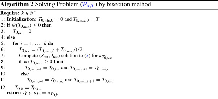

All computations shown in Sect. 3 indicate, as expected, that the optimal trajectories computed by the two methods do coincide.

For illustrative purpose, we provide in Fig. 8 the graph of the cost $j(T_0)$ defined in (18) that corresponds to the one-dimensional optimization Problem ${\tilde{\mathcal{P}}}_{\alpha ,T}$. As can be seen, the cost is not convex.

Fig. 8.

Graph of the cost value j with respect to $T_0$ for $T=200$ (left) and $T=300$ (right)

References

- 1.Abakuks A. An optimal isolation policy for an epidemic. J. Appl. Probab. 1973;10(2):247–262. doi: 10.2307/3212343. [DOI] [Google Scholar]
- 2.Abakuks A. Optimal immunisation policies for epidemics. Adv. Appl. Probab. 1974;6(3):494–511. doi: 10.2307/1426230. [DOI] [Google Scholar]
- 3.Ainseba B, Iannelli M. Optimal screening in structured SIR epidemics. Math. Modell. Nat. Phenom. 2012;7(3):12–27. doi: 10.1051/mmnp/20127302. [DOI] [Google Scholar]
- 4.Alkama M, Elhia M, Rachik Z, Rachik M, Labriji EH. Free terminal time optimal control problem of an SIR epidemic model with vaccination. Int. J. Sci. Res. 2014;3:227. [Google Scholar]
- 5.Greenhalgh, D.: Some results on optimal control applied to epidemics. Math. Biosci. 88(2), 125–158 (1988)
- 6.Andreasen V. The final size of an epidemic and its relation to the basic reproduction number. Bull. Math. Biol. 2011;73(10):2305–2321. doi: 10.1007/s11538-010-9623-3. [DOI] [PMC free article] [PubMed] [Google Scholar]
- 7.Gaff, H., Schaefer, E.: Optimal control applied to vaccination and treatment strategies for various epidemiological models. Math. Biosci. Eng. 6(3), 469 (2009) [DOI] [PubMed]
- 8.Behncke H. Optimal control of deterministic epidemics. Optim. Control Appl. Methods. 2000;21(6):269–285. doi: 10.1002/oca.678. [DOI] [Google Scholar]
- 9.Bliman PA, Duprez M. How best can finite-time social distancing reduce epidemic final size? J. Theor. Biol. 2020;511:110557. doi: 10.1016/j.jtbi.2020.110557. [DOI] [PMC free article] [PubMed] [Google Scholar]
- 10.Bolzoni L, Bonacini E, Soresina C, Groppi M. Time-optimal control strategies in SIR epidemic models. Math. Biosci. 2017;292:86–96. doi: 10.1016/j.mbs.2017.07.011. [DOI] [PMC free article] [PubMed] [Google Scholar]
- 11.Bolzoni L, Bonacini E, Marca RD, Groppi M. Optimal control of epidemic size and duration with limited resources. Math. Biosci. 2019;315:108232. doi: 10.1016/j.mbs.2019.108232. [DOI] [PubMed] [Google Scholar]
- 12.Buonomo B, Manfredi P, d’Onofrio A. Optimal time-profiles of public health intervention to shape voluntary vaccination for childhood diseases. J. Math. Biol. 2019;78(4):1089–1113. doi: 10.1007/s00285-018-1303-1. [DOI] [PubMed] [Google Scholar]
- 13.Buonomo B, Della Marca R, d’Onofrio A. Optimal public health intervention in a behavioural vaccination model: the interplay between seasonality, behaviour and latency period. Math. Med. Biol. A J. IMA. 2019;36(3):297–324. doi: 10.1093/imammb/dqy011. [DOI] [PubMed] [Google Scholar]
- 14.Di Blasio G. A synthesis problem for the optimal control of epidemics. Numer. Funct. Anal. Optim. 1980;2(5):347–359. doi: 10.1080/01630568008816063. [DOI] [Google Scholar]
- 15.Shim, E.: Optimal dengue vaccination strategies of seropositive individuals. Math. Biosci. Eng. 16(3), 1171–1189 (2019) [DOI] [PubMed]
- 16.Gaff H, Schaefer E. Optimal control applied to vaccination and treatment strategies for various epidemiological models. Math. Biosci. Eng. 2009;6(3):469. doi: 10.3934/mbe.2009.6.469. [DOI] [PubMed] [Google Scholar]
- 17.Greenhalgh D. Some results on optimal control applied to epidemics. Math. Biosci. 1988;88(2):125–158. doi: 10.1016/0025-5564(88)90040-5. [DOI] [Google Scholar]
- 18.Hansen E, Day T. Optimal control of epidemics with limited resources. J. Math. Biol. 2011;62(3):423–451. doi: 10.1007/s00285-010-0341-0. [DOI] [PubMed] [Google Scholar]
- 19.Hollingsworth TD, Klinkenberg D, Heesterbeek H, Anderson RM. Mitigation strategies for pandemic influenza A: balancing conflicting policy objectives. PLoS Comput. Biol. 2011;7(2):e1001076. doi: 10.1371/journal.pcbi.1001076. [DOI] [PMC free article] [PubMed] [Google Scholar]
- 20.Hu Q, Zou X. Optimal vaccination strategies for an influenza epidemic model. J. Biol. Syst. 2013;21(04):1340006. doi: 10.1142/S0218339013400068. [DOI] [Google Scholar]
- 21.Morris, D.H., Rossine, F.W., Plotkin, J.B., Levin, S.A.: Optimal, near-optimal, and robust epidemic control. arXiv preprint arXiv:2004.02209 (2020)
- 22.Jaberi-Douraki M, Moghadas SM. Optimality of a time-dependent treatment profile during an epidemic. J. Biol. Dyn. 2013;7(1):133–147. doi: 10.1080/17513758.2013.816377. [DOI] [PMC free article] [PubMed] [Google Scholar]
- 23.Jaberi-Douraki M, Heffernan JM, Wu J, Moghadas SM. Optimal treatment profile during an influenza epidemic. Differ. Equ. Dyn. Syst. 2013;21(3):237–252. doi: 10.1007/s12591-012-0149-z. [DOI] [Google Scholar]
- 24.Katriel G. The size of epidemics in populations with heterogeneous susceptibility. J. Math. Biol. 2012;65(2):237–262. doi: 10.1007/s00285-011-0460-2. [DOI] [PubMed] [Google Scholar]
- 25.Kermack WO, McKendrick AG. Contributions to the mathematical theory of epidemics-I. Proc. R. Soc. 1927;115A:700–721. doi: 10.1007/BF02464423. [DOI] [PubMed] [Google Scholar]
- 26.Jaberi-Douraki, M., Moghadas, S.M.: Optimality of a time-dependent treatment profile during an epidemic. J. Biol. Dyn. 7(1), 133–147 (2013) [DOI] [PMC free article] [PubMed]
- 27.Jaberi-Douraki, M., Heffernan, J.M., Wu, J., Moghadas, S.M.: Optimal treatment profile during an influenza epidemic. Differ. Equ. Dyn. Syst. 21(3), 237–252 (2013)
- 28.Kolesin ID, Zhitkova EM. Optimization of immunocorrection of collective immunity. Autom. Remote Control. 2016;77(6):1031–1040. doi: 10.1134/S0005117916060072. [DOI] [Google Scholar]
- 29.Kolesin, I.D., Zhitkova, E.M.: Optimization of immunocorrection of collective immunity. Autom. Remote Control 77(6), 1031–1040 (2016)
- 30.Laguzet L, Turinici G. Globally optimal vaccination policies in the SIR model: smoothness of the value function and uniqueness of the optimal strategies. Math. Biosci. 2015;263:180–197. doi: 10.1016/j.mbs.2015.03.002. [DOI] [PubMed] [Google Scholar]
- 31.Lee EB, Markus L. Foundations of Optimal Control Theory. New York: Wiley; 1967. [Google Scholar]
- 32.Ma J, Earn DJ. Generality of the final size formula for an epidemic of a newly invading infectious disease. Bull. Math. Biol. 2006;68(3):679–702. doi: 10.1007/s11538-005-9047-7. [DOI] [PMC free article] [PubMed] [Google Scholar]
- 33.Manfredi P, D’Onofrio A. Modeling the Interplay Between Human Behavior and the Spread of Infectious Diseases. Berlin: Springer; 2013. [Google Scholar]
- 34.Angulo, M.T., Castaños, F., Velasco-Hernandez, J.X., Moreno, J.A.: A simple criterion to design optimal nonpharmaceutical interventions for epidemic outbreaks. medRxiv (2020) [DOI] [PMC free article] [PubMed]
- 35.Miller JC. A note on the derivation of epidemic final sizes. Bull. Math. Biol. 2012;74(9):2125–2141. doi: 10.1007/s11538-012-9749-6. [DOI] [PMC free article] [PubMed] [Google Scholar]
- 36.Kermack, W.O., McKendrick, A.G.: Contributions to the mathematical theory of epidemics-I. Proc. R. Soc. 115A, 700–721 (1927) [DOI] [PubMed]
- 37.Morton R, Wickwire KH. On the optimal control of a deterministic epidemic. Adv. Appl. Probab. 1974;6(4):622–635. doi: 10.2307/1426183. [DOI] [Google Scholar]
- 38.Piguillem F, Shi L. The optimal COVID-19 quarantine and testing policies. Einaudi Institute for Economics and Finance (EIEF): Tech. Rep; 2020. [Google Scholar]
- 39.Salje, H., Kiem, C.T., Lefrancq, N., Courtejoie, N., Bosetti, P., Paireau, J., Andronico, A., Hozé, N., Richet, J., Dubost, C.L., et al.: Estimating the burden of SARS-CoV-2 in France. Science (2020) [DOI] [PMC free article] [PubMed]
- 40.Shim E. Optimal dengue vaccination strategies of seropositive individuals. Math. Biosci. Eng. 2019;16(3):1171–1189. doi: 10.3934/mbe.2019056. [DOI] [PubMed] [Google Scholar]
- 41.Wickwire KH. Optimal isolation policies for deterministic and stochastic epidemics. Math. Biosci. 1975;26(3–4):325–346. doi: 10.1016/0025-5564(75)90020-6. [DOI] [Google Scholar]
- 42.Wickwire K. Optimal immunization rules for an epidemic with recovery. J. Optim. Theory Appl. 1979;27(4):549–570. doi: 10.1007/BF00933440. [DOI] [Google Scholar]
- 43.Yang, K., Wang, E., Zhou, Y., Zhou, K.: Optimal vaccination policy and cost analysis for epidemic control in resource-limited settings. Kybernetes (2015)
- 44.Zhou Y, Wu J, Wu M. Optimal isolation strategies of emerging infectious diseases with limited resources. Math. Biosci. Eng. MBE. 2013;10:1691–1701. doi: 10.3934/mbe.2013.10.1691. [DOI] [PubMed] [Google Scholar]