

Abstract
We developed a mathematical model to describe the new coronavirus transmission in São Paulo State, Brazil. The model divided a community into subpopulations composed of young and elder persons considering a higher risk of fatality among elder persons with severe CoViD-19. From the data collected in São Paulo State, we estimated the transmission and additional mortality rates. Based on the estimated model parameters, we calculated the basic reproduction number  , and we retrieved the number of deaths due to CoViD-19, which was three times lower than those found in the literature. Considering isolation as a control mechanism, we varied the isolation rates in the young and elder subpopulations to assess the epidemiological impacts. The epidemiological scenarios focused mainly on evaluating the reduction in the number of severe CoViD-19 cases and deaths due to this disease when isolation is introduced in a population.
Keywords: mathematical model, numerical simulations, SARS-CoV-2/CoViD-19, quarantine/relaxation, epidemiological scenarios
1. Introduction
Coronavirus disease 2019 (CoViD-19) is caused by the severe acute respiratory syndrome coronavirus 2 (SARS-CoV-2, a strain of the SARS-CoV-1 pandemic in 2002/2003) originated in Wuhan, China, in December 2019, and spread out worldwide. The World Health Organization (WHO) declared CoViD-19 pandemic on March 11, 2020, based on its definition: ‘A pandemic is the worldwide spread of a new disease. An influenza pandemic occurs when a new influenza virus emerges and spreads around the world, and most people do not have immunity’.
SARS-CoV-2 (new coronavirus), an RNA virus, can be transmitted by droplets that escape lungs through coughing or sneezing and infects humans (direct transmission) or is deposited in surfaces and infects humans when in contact with this contaminated surface (indirect transmission). This virus enters into a susceptible person through the nose, mouth or eyes, infects cells in the respiratory tract and releases millions of new viruses. In severe cases, immune cells overreact and attack lung cells causing acute respiratory disease syndrome and possibly death. In general, the fatality rate in elder patients (60 years or more) is much higher than in young patients, and under 40 years seems to be around  (WHO, 2020). There is no vaccine, neither efficient treatment, even many drugs (chloroquine, for instance) are under clinical trial. Like all RNA-based viruses, coronavirus tends to mutate faster than DNA viruses but slower than influenza viruses.
Many mathematical and computational models are being used to describe the current new coronavirus pandemic. In mathematical modeling, there is a threshold (see Anderson & May, 1991) called the basic reproduction number denoted by  , which is the secondary cases produced by one case introduced in a completely susceptible population. When a control mechanism is introduced, this number decreases and is called the reduced reproduction number
  . Ferguson et al. (2020) proposed a model to investigate the effects on the CoViD-19 epidemic when susceptible persons are isolated. They analysed two scenarios called mitigation and suppression. Roughly, mitigation decreases the reduced reproduction number
  , but not lower than one (
 ), while suppression decreases the reduced reproduction number lower than one (
 ). They predicted the numbers of severe cases and deaths due to CoViD-19 without control measure and compared them with those numbers when isolation (mitigation and suppression) is introduced as control measures. Li et al. discussed the role of undocumented infections (Li et al., 2020).
In this paper, we formulate a mathematical model based on ordinary differential equations to understand the new coronavirus transmission dynamics and, using the data from São Paulo State, Brazil, to estimate the model parameters. These estimated parameters allow us to study potential scenarios of isolation as a control mechanism.
The paper is structured as follows. In Section 2, we introduce a model, which is numerically studied in Section 3. Discussions are presented in Section 4, and conclusions in Section 5.
2. Material and methods
In a community where the new coronavirus is circulating, the risk of infection is more significant in the elder than in young persons, as well as elder persons are under an increased probability of being symptomatic with higher CoViD-19 induced mortality. Hence, we divide a community into two groups: young (under 60 years old, denoted by subscript  ) and elder (above 60 years old, denoted by subscript
  ) subpopulations. We describe the community’s vital dynamic by the per-capita birth (
 ) and death (
 ) rates.
Each subpopulation  (
( ) is divided into eight classes: susceptible
  , susceptible persons who are isolated
  , exposed (infected but not infectious)
  , asymptomatic
  , asymptomatic caught by test and then isolated
  , pre-diseased (pre-symptomatic, before the onset of CoViD-19)
  , symptomatic but presenting mild CoViD-19 (or non-hospitalized)
  and symptomatic with severe CoViD-19 (hospitalized)
  . Pre-diseased persons caught by test are isolated and, for simplicity, they are transferred to non-transmitting class
  . However, young and elder persons enter into the same immune class
  after experiencing the infection. Table 1 summarizes the model variables.
Table 1.
Summary of the model variables ( ).
).
| Symbol | Meaning | |
|---|---|---|

|
Susceptible persons | |

|
Isolated among susceptible persons | |

|
Exposed (infected but not infectious) persons | |

|
Asymptomatic persons | |

|
Isolated among asymptomatic persons caught by test | |

|
Presymptomatic (pre-diseased) persons | |

|
Isolated among pre-diseased persons caught by test | |

|
Symptomatic (diseased) persons | |

|
Immune (recovered) persons |
We describe the natural history of the new coronavirus infection for the young ( ) and elder (
 ) subpopulations. We assume that only persons in asymptomatic (
 ) and pre-diseased (
 ) classes are transmitting the virus, and other infected classes (
 ,
,  and
and  ) are under voluntary or forced isolation. The susceptible persons in contact with the virus released by asymptomatic and pre-diseased persons can be infected at a rate
  (known as mass action law; Anderson & May, 1991) and enter into class
  , where
  is the per-capita incidence rate (or force of infection) defined by
  , with
  being
being
 |
(1) |
where  is the Kronecker delta, with
  if
if  , and
, and  , if
, if  ; and
; and  and
and  are the transmission rates, i.e. the rates at which virus encounters susceptible person and infects him/her.
Susceptible persons are infected at a rate  and enter into class
  . After an average period
  in class
  , where
  is the incubation rate, exposed persons enter into asymptomatic
  (with probability
  ) or pre-diseased
  (with probability
  ) classes. After an average period
  in class
  , where
  is the infection rate of asymptomatic persons, symptomatic persons acquire immunity and enter into immune (recovered) class
  . Another route of exit from class
  is being caught by test at a rate
  and entering into class
  , and, then, after a period
  , entering into class
  . With very low intensity, asymptomatic persons are in voluntary isolation, described by the voluntary isolation rate
  . For the pre-symptomatic persons, after an average period
  in class
  , where
  is the infection rate of pre-diseased persons, they enter into non-hospitalized
  (with probability
  ) or hospitalized
  (with probability
  ) classes. The pre-symptomatic persons can also be caught by test at a rate
  and enter into class
  . Hospitalized persons acquire immunity after a period
  , where
  is the recovery rate of severe CoViD-19, and enter into immune class
  , or die under disease-induced (additional) mortality rate
  . The severe CoViD-19 cases are also treated at a rate
  and enter into immune class
  . After an average period
  in class
  , non-hospitalized persons acquire immunity and enter into immune class
  , or enter into class
  at a relapsing rate
  .
.
For the control of the CoViD-19 epidemic, we consider continuous isolation and release of persons. We assume that susceptible young and elder persons are removed from susceptible class  at the isolation rate
  , and released from class
  at the release rate
  , with
  .
.
Figure 1 shows the flowchart of the new coronavirus transmission model.
Fig. 1.
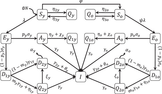
The flowchart of the new coronavirus transmission model with variables and parameters. In all classes, the arrow corresponding to the natural mortality rate  is not shown.
Based on the above descriptions summarized in Fig. 1, the new coronavirus transmission model is described by a system of ordinary differential equations, with  . The equations for susceptible persons are
 |
(2) |
for susceptible persons in isolation  and infected persons are
 |
(3) |
and for immune persons is
 |
(4) |
with  obeying, with
  ,
,
 |
(5) |
where the initial number of population at  is
is  . The initial conditions (at
  ) supplied to equations (2), (3 ) and (4) are
 |
where  is a non-negative number. For instance,
  describes the absence of exposed persons at the beginning of the epidemic.
Table 2 summarizes the model parameters and values (those for elder classes are between parentheses).
Table 2.
Summary of the model parameters ( ) and values (rates in
  , time in
  and proportions are dimensionless). Some values are calculated (
 ), or varied (
 ), or assumed (
 ), or estimated (
 ) or not available (
 ).
).
| Symbol | Meaning | Value | ||
|---|---|---|---|---|

|
Natural mortality rate |
 SEADE–Fundação Sistema Estadual (2020)
|
||

|
Birth rate |
|
||

|
Aging rate |
|
||

|
Incubation rate |
 WHO (2020)
|
||

|
Infection rate of asymptomatic persons |
 WHO (2020)
|
||

|
Infection rate of pre-diseased persons |
 WHO (2020)
|
||

|
Recovery rate of severe CoViD-19 |
 WHO (2020)
|
||

|
Relapsing rate of pre-diseased persons |
|
||

|
Additional mortality rate |
|
||

|
Testing rate among asymptomatic persons |

|
||

|
Voluntary isolation rate of asymptomatic persons |

|
||

|
Testing rate among pre-diseased persons |

|
||

|
Isolation rate of susceptible persons |

|
||

|
Releasing rate of isolated persons |

|
||

|
Treatment rate |

|
||

|
Transmission rate due to asymptomatic persons |

|
||

|
Transmission rate due to pre-diseased persons |
|
||

|
Scaling factor of transmission among elder persons |

|
||

|
Proportion of asymptomatic persons |

|
||

|
Proportion of mild (non-hospitalized) CoViD-19 |
 Boletim Epidemiológico 08 (2020)
|
The isolation of persons deserves some words. In the modeling, we know the number of isolated susceptible persons exactly when introducing the new coronavirus,  . However, as time passes, susceptible persons are infected and acquire immunity, and, due to asymptomatic persons, susceptible and immunized persons are indistinguishable (except when hospitalized or caught by test). For this reason, if isolation of persons is not implemented at the time of the introduction of the virus, this virus should probably be circulating among the isolated population, but at a lower transmission rate (virus spreads restricted among household and neighborhood persons), which is not considered in the model.
From the system of equations (2), (3) and (4), we can derive some epidemiological parameters: new cases, severe CoViD-19 cases, number of deaths due to CoViD-19 and isolated persons.
The numbers of persons infected with the new coronavirus are given by  for young subpopulation, and
  for elder subpopulation. The incidence rates are
 |
(6) |
where the per-capita incidence rate  is given by equation (1), and the numbers of new cases
  and
and  are
are
 |
with  and
and  . The daily numbers of new cases
  and
and  are
are
 |
which are entering into classes  and
and  , where
  ,
, 
 , for
, for  , with
  .
.
The numbers of accumulated severe (hospitalized) CoViD-19 cases  and
and  are given by those exiting from
  ,
,  ,
,  and
and  , i.e.
 |
(7) |
with  and
and  , and the daily numbers of hospitalized cases
  and
and  are
are
 |
which are entering into classes  and
and  .
.
We can calculate the number of accumulated deaths caused by severe CoViD-19 cases  from hospitalized patients and is
 |
(8) |
with  . The daily number of dead persons
  is
is
 |
where  and
and  are the daily numbers of deaths in young and elder subpopulations.
We obtain the number of susceptible persons in isolation in the absence of release  from
from
 |
(9) |
where  and
and  are the numbers of isolated young and elder persons.
The system of equations (2), (3) and (4) is non-autonomous. Nevertheless, the fractions of persons in each compartment approach to a steady state (see Appendix A), hence, by using equations (A.11) and (A.12), the reduced reproduction number  is approximated by
 |
(10) |
where  and
and  are substituted by
  and
and  .
.
Given  and
and  , let us evaluate roughly the threshold number of susceptible persons to trigger and maintain an epidemic, assuming that all model parameters for young and elder subpopulations and all transmission rates are equal. In this special case,
  and
and  , using approximated
  given by equation (A.16). Letting
  , the critical number of susceptible persons
  at equilibrium is
 |
(11) |
If  , epidemic occurs and persists (
 , the non-trivial equilibrium point
  ), and the fraction of susceptible individuals is
  , where
  ; but if
  , epidemic occurs but fades out (
 , the trivial equilibrium point
  ), and the fractions of susceptible individuals
  and
and  at equilibrium are given by equation (A.4) or (A.13) in the absence of controls.
Let us now evaluate roughly the critical isolation rate of susceptible persons  assuming that all model parameters for young and elder subpopulations and all transmission rates are equal. In this particular case,
  , where
  , and letting
  , we obtain
 |
(12) |
If  , the epidemic occurs and persists (
 , the non-trivial equilibrium point
  ); but if
  , the epidemic fades out (
 , the trivial equilibrium point
  ).
).
We apply the above results to study the introduction and establishment of the new coronavirus in São Paulo State, Brazil. From the data collected in São Paulo State from March 14, 2020, until April 5, 2020, we estimate the transmission and additional mortality rates, and, then, we study the potential scenarios introducing isolation as a control mechanism.
3. Results
The results obtained in the preceding section are applied to describe the new coronavirus infection in São Paulo State. The first confirmed case of CoViD-19, on February 26, 2020, was from a traveler returning from Italy on February 21 and being hospitalized on February 24. The first death due to CoViD-19 was a 62 years old male with comorbidity who never traveled abroad, hence considered an autochthonous transmission. He manifested his early symptoms on March 10, was hospitalized on March 14 and died on March 16. On March 24, the São Paulo State authorities ordered the isolation of persons acting in non-essential activities and students of all levels until April 6, which was extended to April 22.
Let us determine the initial conditions. In São Paulo State, the number of inhabitants is  according to SEADE (SEADE–Fundação Sistema Estadual, 2020). We calculate the value of parameter
  given in Table 1 using equation (A.13), i.e.
  , where
  is the proportion of elder persons. Using
  in São Paulo State (SEADE–Fundação Sistema Estadual, 2020), we obtained
 , hence,
  (
( ) and
) and  (
( ). The initial conditions for susceptible persons are let to be
  and
and  . For other variables, using
  and
and  from Table 2, the ratios asymptomatic:symptomatic and mild:severe (non-hospitalized:hospitalized) CoViD-19 are 4:1. To set up initial conditions, we may use as an approximation these same ratios for elder persons, even though
  and
and  are slightly different. Hence, if we assume that there is one person in
  (the first confirmed case in the elder subpopulation), then there are four persons in
  . The sum 5 is the number of persons in class
  , implying that there are 20 in class
  ; hence, the sum 25 is the number of persons in class
  . Finally, we suppose that no one is isolated or tested and also immunized. We assume that the young subpopulation’s initial conditions are equal to those assigned to the elder subpopulation. (Probably the first confirmed CoViD-19 person transmitted the virus (since February 21 when returned infected from Italy), as well as other asymptomatic travelers returning from abroad, and, perhaps, a young person with severe CoViD-19 was wrongly diagnosed as SARS.)
Therefore, the initial conditions supplied to the dynamic system (2), (3) and (4) are
 |
where the initial simulation time  corresponds to the calendar time February 26, 2020, when the first case was confirmed. This system is evaluated numerically using fourth-order Runge–Kutta method.
In this section, we present the estimation of the model parameters and the natural epidemic scenario (section 3.1), the epidemiological scenarios with isolation (section 3.2) and the epidemiological scenarios of relaxation (section 3.3).
3.1 Parameters estimation and the natural epidemic
Here we present parameters estimation and epidemiological scenario of the natural epidemic, i.e. the transmission of the new coronavirus without any control. For simplicity, we assume that all transmission rates in the young subpopulation are equal, as well as in the elder subpopulation, i.e. we assume that
 |
hence the forces of infection are  and
and  .
.
Currently, the number of kits to detect the infection by the new coronavirus is insufficient. For this reason, only hospitalized persons and those who died manifesting symptoms of CoViD-19 are tested to confirm the infection by SARS-CoV-2. Hence, we have only observed data of hospitalized persons ( and
and  ) and those who died (
 and
and  ). Taking into account hospitalized persons with CoViD-19, we estimate the transmission rates, and from persons who died due to CoViD-19, we estimate the additional mortality rates, which are estimated by applying the least square method (see Raimundo et al., 2002).
The effects of quarantine at  , corresponding to calendar time on March 24, are expected to appear later. Hence, we will estimate the parameters taking into account the confirmed cases and deaths from February 26 (
 ) to April 5 (
 ),1 hence
  observations. We expect that at around simulation time
  (April 10), the effects of isolation will appear (the sum of the incubation and recovery periods (see Table 2) is around 16 days).
To estimate the transmission rates  and
and  , we let
  and the system of equations (2), (3) and (4) is evaluated, and we calculate
 |
(13) |
where  stands for the minimum value,
  is the number of observations,
  is
is  -th observation time,
  and
and  are given by equation (7) and
  and
and  are the observed number of accumulated CoViD-19 cases.
To estimate the mortality rates  and
and  , we fix previously estimated transmission rates
  and
and  and the system of equations (2), (3) and (4) is evaluated, and we calculate
 |
(14) |
where  stands for minimum value,
  is the number of observations,
  is
is  -th observation time,
  and
and  are given by equation (8) and
  and
and  are the observed number of dead persons.
3.1.1 Estimation of the transmission and additional mortality rates
Firstly, letting the additional mortality rates equal to zero ( ), we estimate a unique
  , with
  , against hospitalized CoViD-19 cases (
 ) collected from São Paulo State. The estimated value is
 , resulting, for the basic reproduction number,
  (partials
  and
and  ) using equation (A.14). Around this value, we vary
  and
and  and choose the better-fitted values comparing the curve of
  with the observed data. The estimated values are
  and
and  (
( ), where
  , resulting in the basic reproduction number
  (partials
  and
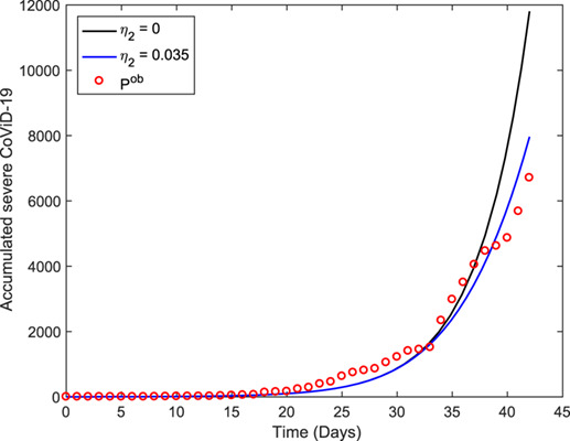
and  ). Figure 2 shows the estimated curve of
  and the observed data. This estimated curve is quite the same as the curve fitted using a unique
  .
.
Fig. 2.
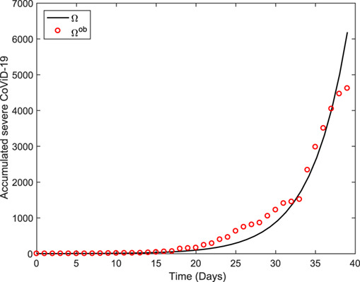
The estimated accumulated severe CoViD-19 cases  and the observed data. The estimated transmission parameters are
  and
and  (
( ).
).
We fix the transmission rates  and
and  (both
(both  ), and we estimate the additional mortality rates
  and
and  . We vary
  and
and  and choose the better-fitted values comparing the curve of deaths due to CoViD-19
  with the observed data. By the fact that lethality in the young subpopulation is much lower than in the elder subpopulation, we let
  (WHO, 2020) and fit only one variable
  . The estimated rates are
  and
and  (
( ). Figure 3 shows the estimated curve of
  and the observed data. We call this the first estimation method.
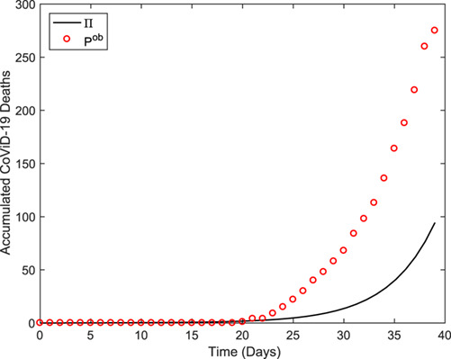
Fig. 3.
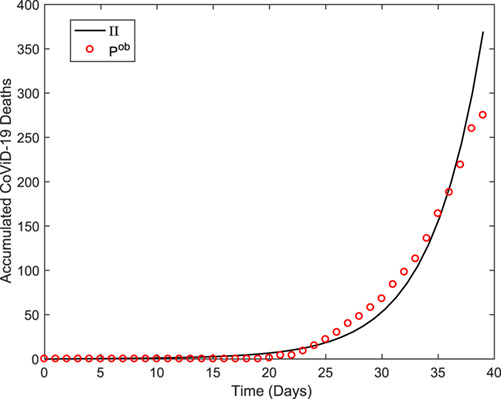
The estimated curve of the accumulated deaths due to CoViD-19  and the observed data. The estimated additional mortality rates are
  and
and  (
( ) for the first estimation method.
The first estimation method used only one information: the risk of death is higher in the elder than young subpopulation (we used  ). However, the lethality among hospitalized elder persons is
  (Boletim Epidemiológico 08, 2020). Combining both findings, we assume that the numbers of deaths in the young and elder subpopulations are, respectively,
  and
and  of the accumulated cases when
  and
and  approach plateaus (see Fig. 5 below). This procedure is called the second estimation method, which considers the second information besides that used in the first estimation method. In this procedure, the estimated rates are
  and
and  (
( ). Figure 4 shows the estimated curve
  and the observed data, which fits the initial phase of the epidemic very badly, but estimates reasonably the number of deaths at the end of the epidemic (see Fig. 6 below).
Fig. 5.
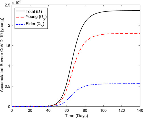
The estimated curves of the accumulated number of severe CoViD-19 ( ,
,  and
and  ) during the first wave of the epidemic.
Fig. 4.
The estimated curve of the accumulated deaths due to CoViD-19  and the observed data. The estimated additional mortality rates are
  and
and  (
( ) for the second estimation method.
Fig. 6.
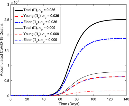
The estimated curves of the accumulated number of CoViD-19 deaths ( ,
,  and
and  ) during the first wave of the epidemic, for the first (thick curves, labeled
  ) and the second (thin curves, labeled
  ) methods of estimation.
Reliable estimations of both transmission and additional mortality rates are crucial for predicting new cases (to adequate the number of beds in hospitals and ICUs, for instance) and deaths. When the estimation is based on a small number of data, i.e. at the beginning of the epidemic, we must take some cautions because the rates may be over or underestimated. At the very beginning phase of the epidemic, the spreading out of infection and deaths increase exponentially. Remember that the estimated parameters, especially the additional mortality rates, were based only on 40 observed data. It is worth stressing that further data will be influenced by the isolation implemented in São Paulo State, and the epidemic curve will follow a decreased trend departing from the natural epidemic.
The fitted parameters  ,
,  ,
,  and
and  are fixed, and the control variables
  and
and  are varied, aiming to obtain the epidemiological scenarios. In general, the epidemic period of infection by viruses is around 2 years, and depending on the value of
  , a second epidemic occurs after elapsed many years (Yang, 1998). For this reason, we study the epidemiological scenarios of CoViD-19 restricted during the first wave of the epidemic, which is around
  days.
days.
Remembering that human population is varying due to the additional mortality (fatality) of severe CoViD-19, we have, at  (calendar time, February 26),
  ,
,  and
and  , and at
  days (calendar time, August 24),
  (
( ),
),  (
( ) and
) and  (
( ) for the first estimation method, and
  (
( ),
),  (
( ) and
) and  (
( ) for the second estimation method. The percentage of deaths (
 ) is given between parentheses.
3.1.2 Natural epidemiological scenario
To describe the entire first wave of the natural epidemic of CoViD-19, we extend the estimated curves until  days, when the epidemic attains low values. We refer to the severe CoViD-19
  as the epidemic curve (notice that the epidemic curve can be defined in several ways, for instance, the sum of those manifesting CoViD-19
  ).
).
Figure 5 shows the extended curves of the accumulated number of severe CoViD-19 ( ,
,  and
and  ) shown in Fig. 2, using equation (7). At
  days (calendar time, July 15),
  approached an asymptote (or a plateau), which can be understood as the time when the first wave of the epidemic ends. Instead of
  days, the curves
  ,
,  and
and  attain values at
  days, respectively,
  ,
,  and
and  .
.
Figure 6 shows the extended curves of the accumulated number of CoViD-19 deaths ( ,
,  and
and  ) shown in Figs 3 and 4, using equation (8). At
  days,
days,  approached a plateau. The values of
  ,
,  and
and  at
at  days for the first method of estimation (thick curves, labeled
  ) are, respectively,
  (
( ),
),  (
( ) and
) and  (
( ), and for the second method of estimation (thin curves, labeled
  ), respectively,
  (
( ),
),  (
( ) and
) and  (
( ). The percentage between parentheses is the ratio
  .
.
By comparing the percentages of fatalities due to CoViD-19 ( ), the first method predicted a higher number of deaths than that predicted by the second method. The second method predicted deaths in
  of the severe CoViD-19, three times lower than
  predicted by the first method, especially in the elder subpopulation. Hence, the second estimation is more credible than the first one, and we adopt hereafter the values provided by the second estimation method for additional mortality rates,
  and
and  (
( ), except when explicitly cited. Remember that the additional mortality rates are considered constant at all times.
Based on the estimated transmission and additional mortality rates, we solve numerically the system of equations (2), (3) and (4) to obtain the natural epidemiological scenario.
Figure 7 shows the estimated natural epidemic curves of CoViD-19 ( ,
,  and
and  ). We observe that the peaks of severe CoViD-19 for elder, young and entire populations are, respectively,
  ,
,  , and
, and  , which co-occur at
  days, which corresponds to calendar time May 8.
Fig. 7.
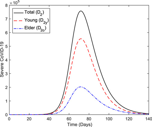
The estimated epidemic curves ( ,
,  and
and  ) during the first wave of the epidemic.
Figure 8 shows the curves of the number of susceptible persons ( ,
,  and
and  ). At
). At  , the numbers of
  ,
,  and
and  are, respectively,
  ,
,  and
and  , which diminish to lower values at
  days due to the infection. Notice that, after the first wave of the epidemic, very few numbers of susceptible persons are left behind, which are
  (
( ),
),  (
( ) and
) and  (
( ), for young, elder and entire populations, respectively. The percentage between parentheses is the ratio
  .
.
Fig. 8.
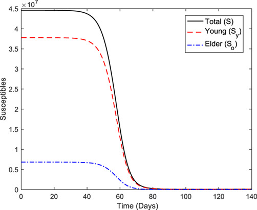
The curves of the number of susceptible persons ( ,
,  and
and  ) during the first wave of the epidemic.
Figure 9 shows the curves of the number of immune persons ( ,
,  and
and  ). The number of immune persons
  ,
,  and
and  increase from zero (
 ) to, respectively,
  (
( ),
),  (
( ) and
) and  (
( ) at
) at  days. The percentage between parentheses is the ratio
  .
.
Fig. 9.
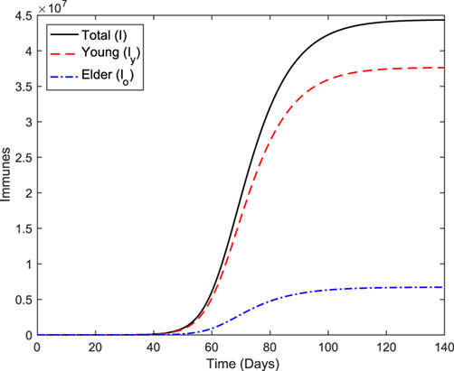
The curves of the number of immune persons ( ,
,  and
and  ) during the first wave of the epidemic.
From Figs 8 and 9, the difference between percentages of  and
and  is the percentage of all persons who harbor the new coronavirus. Hence, the second wave of the epidemic will be triggered after elapsed a very long period of waiting for the accumulation of susceptible persons to surpass its critical number (Yang, 1998, 2001). Simulating the system of equations (2), (3) and (4) for a very long time (figures not shown), the trajectories reach the equilibrium fractions, and for susceptible persons we have
  ,
,  and
and  .
.
Let us estimate roughly the critical number of susceptible persons  from equation (11). For
  , we have
  . Hence, for São Paulo State, isolating
  million (
 ) or above persons is necessary to avoid the epidemic’s outbreak. The number of young persons is
  million, less than the threshold number of isolated persons to guarantee the eradication of the CoViD-19 epidemic. Another rough estimation is for the isolation rate of susceptible person
  , letting
  in equation (12), resulting in
 , for
, for  . Hence, for
  the new coronavirus transmission fades out.
In the next sections, we compare the effects of isolation and relaxation with the natural epidemic of CoViD-19. In the following epidemiological scenarios of isolation and relaxation, we fix the estimated transmission rates,  and
and  (
( ), and the additional mortality rates,
  and
and  (
( ). At the beginning of the CoViD-19 epidemic, only hospitalized persons are tested because the number of testing kits is minimal; hence we let
  , with
  . We neglect the voluntary isolation of asymptomatic persons allowing
  . Also, a vaccine is not available as well as effective treatments, so
  .
.
Using the estimated transmission and additional mortality rates and the values for the model parameters given in Table 2, we solve the system of equations (2), (3) and (4) numerically considering only one control mechanism, i.e. the isolation. Initially, we study the isolation without the subsequent release of isolated persons. After that, we study the relaxation of isolation (release of the isolated persons). By varying isolation parameters  and
and  , and release parameters
  and
and  , we present some epidemiological scenarios. In all scenarios,
  is the simulation time instead of calendar time.
3.2 Epidemiological scenarios of isolation without relaxation ( )
)
At  (February 26), the first case of severe CoViD-19 was confirmed, and at
  (March 24), São Paulo State introduced the isolation as a mechanism of control (described by
  and
and  ) until April 22. We analyse two cases. Initially, there is indiscriminate isolation of young and elder persons, and we assume that the same rates of isolation are applied to young and elder subpopulations, i.e.
  . Further, we deal with a discriminated (preferential) isolation of young or elder persons, then we assume
  .
.
3.2.1 Regime 1–Equal isolation in young and elder subpopulations ( )
)
In regime 1, we consider an equal rate of isolation in the young and elder subpopulations. Notice that  and
and  are per-capita rates, then young and elder persons are isolated proportionally when
  , but the actual number of isolation is higher in the young subpopulation.
We choose seven different values for the isolation rate  (
( ) applied to young and elder subpopulations:
  (
( ),
),  (
( ),
),  (
( ),
),  (
( ),
),  (
( ),
),  (
( ) and
) and  (
( ). The reduced reproduction number
  is calculated using equation (10). For
  , the reduced reproduction number in comparison with the basic reproduction number is decreased to
  . In all figures, the case
  (
( ) is also shown (see Fig. 7).
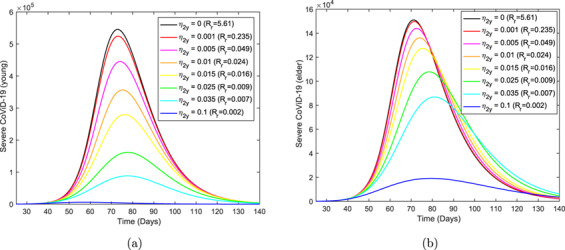
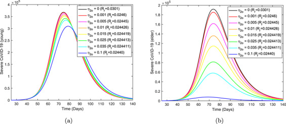
Figure 10 shows the epidemic curves  , for young (a) and elder (b) subpopulations, without and with isolation for different values of
  . Notice that the first two curves obtained with
  and
and  practically coincide, and the latter is slightly lower than the roughly estimated
 . We present the value of the epidemic peak for three values of
  . For
. For  , the peak of the epidemic in the young (first coordinate) and elder (second coordinate) subpopulations are (
 ,
, ), for
  we have (
 ,
, ), and for
  , (
, ( ,
, ). The time (in
  ) at which the peak of the epidemic occurs in the young (first coordinate) and elder (second coordinate) subpopulations for
  ,
,  , and
, and  are, respectively, (
 ,
, ), (
), ( ,
,  ) and (
 ,
, ). For
  in comparison with
  , the epidemic peaks are reduced to
  and
and  , respectively, for young and elder subpopulations. For
  , the peaks are reduced to
  and
and  .
.
Fig. 10.
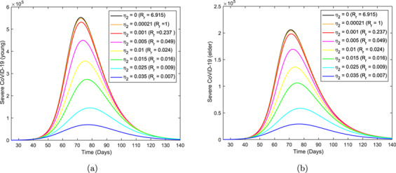
The epidemic curves  ,
,  , without and with isolation for different values of
  . Curves from top to bottom correspond to the increasing
  .
.
As the isolation parameter  increases, the diminished peaks of the curves
  and
and  displace initially to the right (higher times), but at
  , they change the direction and move leftward. However, all curves remain inside the curve without isolation (
 ). The values at which the peaks change direction are
 (
( ) and
) and 
 (
( ). In order to understand this phenomenon, we recall an age-structured model describing the rubella infection (Yang, 1999a,b). As the vaccination rate increases, the peaks of the age-depending force of infection initially move to the right and, then, move leftward.
At  days, isolation began in São Paulo State. For this reason, in the system of equations (2), (3) and (4), we let
  for
for  , and
, and  for
for  . Figure 11 shows the accumulated curves of severe CoViD-19 cases
  without (
 ) and with (
 ) isolation introduced at
  days. The epidemic curve under the isolation bifurcates from the natural epidemic and situates below this curve. It seems that the effects of isolation (in the observed data) appear at around
  (April 5), 11 days after its implementation. The transition from without to with isolation is under very complex dynamics, and, for this reason, we cannot assure that
 is a good estimation (there are so few data). Hence, one of the curves shown in Fig. 10 may correspond to the isolation applied to São Paulo State.
Fig. 11.
The curve of an isolation scheme described by 
 introduced at
  days, and the curve without isolation.
The curve corresponding to 
 in Fig. 10 can be considered as a failure of isolation (
 ) and, for this reason, this curve is removed in all following figures.
Figure 12 shows the curves of accumulated cases of severe CoViD-19  , for young (a) and elder (b) subpopulations, without and with isolation for different values of
  . As the isolation rate
  increases, the accumulated number of severe CoViD-19 cases
  decreases. For instance, at
  days, for
  , the accumulated numbers of patients in the young (first coordinate) and elder (second coordinate) subpopulations are (
 ,
, ), for
  we have (
 ,
, ), and for
  , (
, ( ,
, ). For
  in comparison with
  , the numbers of severe CoViD-19 cases are reduced to
  and
and  , respectively, for young and elder subpopulations. For
  , severe CoViD-19 cases are reduced to
  and
and  .
.
Fig. 12.
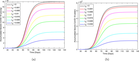
The curves of the accumulated number of severe CoViD-19  ,
,  , without and with isolation for different values of
  . Curves from top to bottom correspond to the increasing
  . The beginning of the isolation occurs at
  days.
days.
Figure 13 shows the curves of accumulated deaths due to CoViD-19  , for young (a) and elder (b) subpopulations, without and with isolation for different values of
  . At
. At  days, for
  , the accumulated numbers of deaths in the young (first coordinate) and elder (second coordinate) subpopulations are (
 ,
, ), for
  we have (
 ,
, ), and for
  , (
, ( ,
, ). For
  , in comparison with
  , the numbers of fatalities due to CoViD-19 are reduced to
  and
and  , respectively, for young and elder subpopulations. For
  , deaths due to CoViD-19 cases are reduced to
  and
and  .
.
Fig. 13.
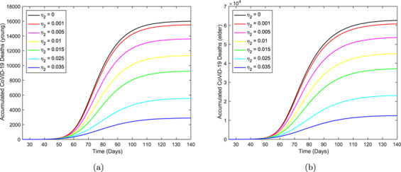
The curves of the accumulated number of CoViD-19 deaths  ,
,  , without and with isolation for different values of
  . Curves from top to bottom correspond to the increasing
  . The beginning of the isolation occurs at
  days.
days.
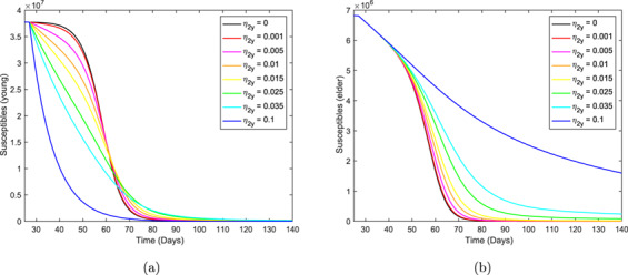
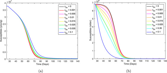
Figure 14 shows the curves of the number of susceptible persons  , for young (a) and elder (b) subpopulations, without and with isolation for different values of
  . At
. At  days, for
  , the numbers of susceptible young (first coordinate) and elder (second coordinate) persons are (
 ,
, ), for
  we have (
 ,
, ), and for
  , (
, ( ,
, ). For
  in comparison with
  , the susceptible persons are decreased to
  and increased to
  , respectively, for young and elder subpopulations. For
  , the susceptible persons are decreased to
  and increased to
  , respectively, for young and elder subpopulations.
Fig. 14.
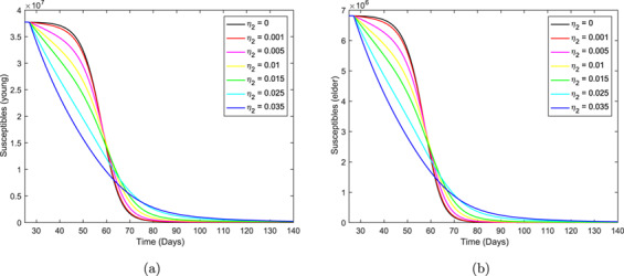
The curves of the number of susceptible persons  ,
,  , without and with isolation for different values of
  . Curves from top to bottom correspond to the increasing
  . The beginning of the isolation occurs at
  days.
days.
As the isolation parameter  increases, the number of susceptible persons decreases according to a sigmoid shape, but they follow exponential decay at a sufficiently higher value. Again, this phenomenon is understood recalling the rubella transmission model (Yang, 2001). As the vaccination rate increases, the fraction of susceptible persons decreases following damped oscillations when
  , attaining the non-trivial equilibrium point. However, for
  , the trivial equilibrium point is an attractor, and the trajectories follow two patterns: (a) if
  is not so low, the fraction of susceptible persons decreases to lower values than the trivial equilibrium point and takes increasing trend to attain the equilibrium value, but not surpassing it (then there is not damped oscillations); and (b) if
  is low, the fraction of susceptible persons decays exponentially and tends to the equilibrium point.
Figure 15 shows the curves of the number of isolated susceptible persons  , for young (a) and elder (b) subpopulations, for different values of
  , from equation (9). At
  days, for
  , there are not isolated persons, for
  , the numbers of isolated young (first coordinate) and elder (second coordinate) persons are (
 ,
, ), and for
  , (
, ( ,
, ). For
  , compared with all persons
  (at
(at  ), isolated susceptible persons are
  and
and  of
of  , respectively, for young and elder persons. For
  , isolated susceptible persons are
  and
and  .
.
Fig. 15.
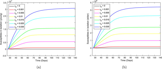
The curves of the number of isolated susceptible persons  ,
,  , with isolation for different values of
  . Curves from top to bottom correspond to the increasing
  . The beginning of the isolation occurs at
  days.
days.
Figure 16 shows the curves of the number of immune persons  , for young (a) and elder (b) subpopulations, without and with isolation for different values of
  . At
. At  days, for
  , the numbers of immune in the young (first coordinate) and elder (second coordinate) subpopulations are (
 ,
, ), for
  we have (
 ,
, ), and for
  , (
, ( ,
, ). For
  , in comparison with
  , the immune persons are reduced to
  and
and  , respectively, for young and elder subpopulations, very close to the reductions observed in the number of deaths due to CoViD-19. For
  , immune persons are reduced to
  and
and  .
.
Fig. 16.
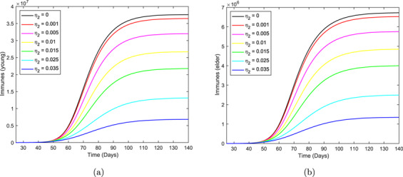
The curves of the number of immunized persons  ,
,  , without and with isolation for different values of
  . Curves from top to bottom correspond to the increasing
  . The beginning of the isolation occurs at
  days.
days.
Epidemiological parameters (peak of  ,
,  ,
,  and
and  ) are reduced quite similarly for
 , i.e. between
  times (
 ) and
) and  times (
 ); however, the number of susceptible persons left behind at the end of the first wave increases less, i.e. two times (young) and three times (elder).
3.2.2 Regime 2–Different isolation in young and elder subpopulations ( )
)
In regime 2, we consider the different rates of isolation in young and elder subpopulations. We fix the isolation rate in the elder subpopulation and vary the young subpopulation’s isolation rate, and vice versa.
Firstly, we choose the isolation rate in the elder subpopulation 
 and vary
  (
( ),
),  (
( ),
),  (
( ),
),  (
( ),
),  (
( ),
),  (
( ) and
) and  (
( ). The reduced reproduction number
  is calculated using equation (10 ).
Figure 17 shows the epidemic curves  , for young (a) and elder (b) subpopulations, fixing
 and varying
  . The decreasing pattern in curve
  follows that observed in regime 1. Still, in the pattern of the curve
  , as
, as  increases, the epidemic peaks displace faster to the right. The curves become more asymmetric (increased skewness) and spread beyond the curve without isolation.
Fig. 17.
The epidemic curves  ,
,  , varying
  , but fixing
 . Curves from top to bottom correspond to the increasing
  . The beginning of the isolation occurs at
  days.
days.
Figure 18 shows the curves of the number of susceptible persons  , for young (a) and elder (b) subpopulations, varying
  , fixing
 . The decreasing pattern of
  follows that observed in regime 1 (sigmoid shape followed by exponential decay). Still, the decreasing sigmoid shaped curves of
  , as
, as  increases, move from bottom to top, which is an opposite pattern to that observed in regime 1. As the isolation in the young subpopulation increases, the number of susceptible young persons decreases, but the number of susceptible elder persons increases. However, from Fig. 17, severe CoViD-19 cases drop for both subpopulations. This can be explained by the decrease in the number of immunized persons: young immune persons decrease
  times when
  decreases from
  to
to  , while elder persons decrease
  times (see Table 3). When
  , the susceptible elder persons approach an asymptote at
  days (calendar time, July 10, 2021).
Fig. 18.
The curves of the number of susceptible persons  ,
,  , varying
  , but fixing
 . Curves from top to bottom correspond to the decreasing
  . The beginning of the isolation occurs at
  days.
days.
Table 3.
Values and percentages of  ,
,  ,
,  and
and  at time
 fixing
 and varying
  ,
,  and
and  (
( ).
).  ,
,  and
and  stand for, respectively, young, elder and total persons.

|

|

|
|||||||
|---|---|---|---|---|---|---|---|---|---|

|

|

|

|

|

|

|

|

|
|

|

|

|

|

|

|

|

|

|

|

|

|

|

|

|

|

|

|

|

|

|

|

|

|

|

|

|

|

|

|

|

|

|

|

|

|

|

|

|

|

|

|

|

|

|

|

|

|

|

|

|

|

|

|

|

|

|

|

|

|

|

|

|

|

|

|

|

|

|

|

|

|

|

|

|

|

|

|

|

|

|

|

|

|

|

|

|

|

|

|

|

|

|

|

|

|

|

|

|

|
The curves of the accumulated number of severe CoViD-19  , the accumulated number of CoViD-19 deaths
  , the number of isolated susceptible person
  and the number of immune persons
  are similar to those shown in the preceding section. For this reason, we present in Table 3 (
 fixed) their values at
  days for young, elder and entire populations, letting
  ,
,  and
and  (
( ). For
  , we have, from the preceding section,
  ,
,  and
and  ;
;  ,
,  and
and  ;
;  ,
,  and
and  ; and
; and  ,
,  and
and  . The percentages are calculated as the ratio between epidemiological parameter evaluated with (
 ) and without (
 ) isolation, at
  . The number of isolated susceptible persons is
  in the absence of the isolation, and the percentage is calculated as the ratio between
  at
at  and
and  .
.
Figures 17 and 18 and Table 3 portray variable isolation in the young subpopulation but maintaining elder persons isolated at a fixed level. Hence, the increase in  protects young persons, but elder persons are also benefited.
Now, we choose the isolation rate in the young subpopulation 
 and vary the isolation rate in the elder subpopulation
  (
( ) for seven different values:
  (
( ),
),  (
( ),
),  (
( ),
),  (
( ),
),  (
( ),
),  (
( ) and
) and  (
( ).
).
Figure 19 shows the epidemic curves  , for young (a) and elder (b) subpopulations, varying
  , but fixing
 . The pattern is similar to that observed in Fig. 7, but changing the pattern of
  by
by  , and vice versa, and more smooth.
Fig. 19.
The epidemic curves  ,
,  , varying
  , but fixing
 . Curves from top to bottom correspond to the increasing
  . The beginning of the isolation occurs at
  days.
days.
Figure 20 shows the curves of the number of susceptible persons  , for young (a) and elder (b) subpopulations, varying
  , but fixing
 . The pattern is similar to that observed in Fig. 18, but changing the pattern of
  by
by  , and vice versa.
Fig. 20.
The curves of the number of susceptible persons  ,
,  , varying
  , but fixing
 . Curves from top to bottom correspond to decreasing
  . The beginning of the isolation occurs at
  days.
days.
The curves of the accumulated number of severe CoViD-19  , the accumulated number of CoViD-19 deaths
  , the number of isolated susceptible person
  and the number of immunized persons
  are similar to those shown in the preceding section. For this reason, we present in Table 4 (
 fixed) their values at
  days for young, elder and entire populations, letting
  ,
,  and
and  (
( ). Values for
  ,
,  ,
,  and
and  , for
, for  , are those used in Table 3, as well as the definitions of the percentages.
Table 4.
Values and percentages of  ,
,  ,
,  and
and  at time
 fixing
 and varying
  ,
,  and
and  (
( ).
).  ,
,  and
and  stand for, respectively, young, elder and total persons.

|

|

|
|||||||
|---|---|---|---|---|---|---|---|---|---|

|

|

|

|

|

|

|

|

|
|

|

|

|

|

|

|

|

|

|

|

|

|

|

|

|

|

|

|

|

|

|

|

|

|

|

|

|

|

|

|

|

|

|

|

|

|

|

|

|

|

|

|

|

|

|

|

|

|

|

|

|

|

|

|

|

|

|

|

|

|

|

|

|

|

|

|

|

|

|

|

|

|

|

|

|

|

|

|

|

|

|

|

|

|

|

|

|

|

|

|

|

|

|

|

|

|

|

|

|

|
Figures 19 and 20 and Table 4 portray variable isolation in the elder subpopulation but maintaining young persons isolated at a fixed level. Hence, the increase in  of course protects elder persons, but young persons are also benefited.
Tables 3 and 4 allow us to choose a suitable isolation scheme aiming at two different goals. If the objective is diminishing the accumulated number of severe CoViD-19 cases  , the best strategy is isolating more young than elder persons. However, if the goal is to reduce the fatality cases
  , the best strategy is isolating more elders than young persons. But, when very intense isolation is possible (
 ), then isolating more young persons is recommended. Notice that only the strategies
  and
and  attain the number of isolated susceptible persons above the threshold
  .
.
The peak of the epidemic in the absence of isolation in São Paulo State occurs around May 8. However, depending on the intensity of the isolation, the peak is displaced at most 8 days later.
3.3 Epidemiological scenarios of relaxation
When the relaxation (release of the isolated persons) begins, equation (9) is not valid anymore to evaluated the accumulated number of isolated susceptible persons. Hence, we use  ,
,  and
and  for the numbers of isolated susceptible, respectively, young, elder and entire populations.
  and
and  are solutions of the system of equations (2), (3) and (4).
At  , the first case of severe CoViD-19 was confirmed, and at
  , São Paulo State introduced the isolation as a mechanism of control (described by
  and
and  ) until April 22.2 Hence, the beginning of the relaxation of isolated persons will occur at the simulation time
  (calendar time, April 22).3 We assume that the same rates of the release are applied to young and elder subpopulations, i.e.
  , and we consider regime 1-type isolation, i.e.
  . Hence, from time
  to
to  , we have
  (without isolation), followed by regime 1-type isolation from
  to
to  with
with  , and since after time
  , we have the isolation and relaxation with the value of
  depending on
  .
.
In order to assess the epidemiological scenarios when isolated persons are released, we fix  (
( ), and vary
  (
( ),
),  (
( ),
),  (
( ),
),  (
( ),
),  (
( ),
),  (
( ) and
) and  (
( ). The reduced reproduction number
  is calculated using equation (10).
Figure 21 shows the epidemic curves  , for young (a) and elder (b) subpopulations, fixing
 , and varying
  . The beginning of release occurs at
  days, the date proposed by the São Paulo State authorities. The epidemic peaks when
 , for young and elder subpopulations are, respectively,
  and
and  , which occur at
  (calendar time, June 4) and
  days.
days.
Fig. 21.
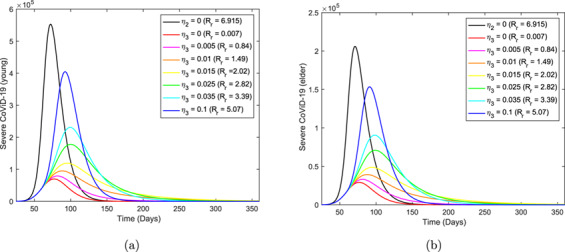
The epidemic curves  ,
,  , fixing
 , and varying
  . Curves from top to bottom correspond to the decreasing
  . The beginning of the release occurs at
  days.
days.
The curves of the accumulated number of severe CoViD-19  , the accumulated number of CoViD-19 deaths
  , the number of isolated susceptible person
  and the number of immune persons
  are similar to those shown in the preceding section. For this reason, we present in Table 5 (
 fixed) their values at
  (calendar time, February 20, 2021) for young, elder and entire populations, letting
  ,
,  and
and  (
( ). For
  , the values of
  ,
,  ,
,  and
and  are those used in Table 3, as well as the definitions of the percentages.
Table 5.
Values and percentages of  ,
,  ,
,  and
and  at time
 fixing
 and varying
  ,
,  and
and  (
( ).
).  ,
,  and
and  stand for, respectively, young, elder and total persons. Releasing initiates at
  .
.

|
|

|
|||||||
|---|---|---|---|---|---|---|---|---|---|

|

|

|

|

|

|

|

|

|
|

|

|

|

|

|

|

|

|

|

|

|

|

|

|

|

|

|

|

|

|

|

|

|

|

|

|

|

|

|

|

|

|

|

|

|

|

|

|

|

|

|

|

|

|

|

|

|

|

|

|

|

|

|

|

|

|

|

|

|

|

|

|

|

|

|

|

|

|

|

|

|

|

|

|

|

|

|

|

|

|

|

|

|

|

|

|

|

|

|

|

|

|

|

|

|

|

|

|

|

|
Figure 22 shows the epidemic curves  , for young (a) and elder (b) subpopulations, fixing
 , and varying
  . The beginning of release is at
  , a week earlier. The epidemic peaks when
 , for young and elder subpopulations are, respectively,
  and
and  , which occur at
  and
and  . In comparison with Fig. 21, the epidemic peaks are increased for young and elder subpopulations by, respectively,
  and
and  , which are anticipated in
  days.
days.
Fig. 22.
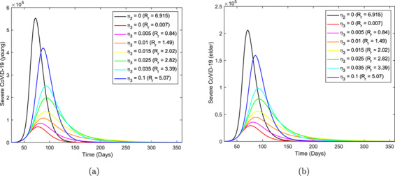
The epidemic curves  ,
,  , fixing
 , and varying
  . Curves from top to bottom correspond to the decreasing
  . The beginning of the release occurs at
  days.
days.
The curves of the accumulated number of severe CoViD-19  , the accumulated number of CoViD-19 deaths
  , the number of isolated susceptible person
  and the number of immune persons
  are similar to those shown in the preceding section. For this reason, we present in Table 6 (
 fixed) their values at
  for young, elder and entire populations, letting
  ,
,  and
and  (
( ). For
  , the values of
  ,
,  ,
,  and
and  are those used in Table 3, as well as the definitions of the percentages.
Table 6.
Values and percentages of  ,
,  ,
,  and
and  at time
 fixing
 and varying
  ,
,  and
and  (
( ).
).  ,
,  and
and  stand for, respectively, young, elder and total persons. Releasing initiates at
  .
.

|

|

|
|||||||
|---|---|---|---|---|---|---|---|---|---|

|

|

|

|

|

|

|

|

|
|

|

|

|

|

|

|

|

|

|

|

|

|

|

|

|

|

|

|

|

|

|

|

|

|

|

|

|

|

|

|

|

|

|

|

|

|

|

|

|

|

|

|

|

|

|

|

|

|

|

|

|

|

|

|

|

|

|

|

|

|

|

|

|

|

|

|

|

|

|

|

|

|

|

|

|

|

|

|

|

|

|

|

|

|

|

|

|

|

|

|

|

|

|

|

|

|

|

|

|

|
Figure 23 shows the epidemic curves  , for young (a) and elder (b) subpopulations, fixing
 , and varying
  . The beginning of release is at
  , a week later. The epidemic peaks when
 are for young and elder subpopulations, respectively,
  and
and  , which occur at
  (calendar time, June 13) and
  . In comparison with Fig. 21, the epidemic peaks are decreased for young and elder subpopulations by, respectively,
  and
and  , which are delayed in
  days.
days.
Fig. 23.
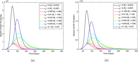
The epidemic curves  ,
,  , fixing
 , and varying
  . Curves from top to bottom correspond to the decreasing
  . The beginning of the release occurs at
  days.
days.
The curves of the accumulated number of severe CoViD-19  , the accumulated number of CoViD-19 deaths
  , the number of isolated susceptible person
  and the number of immune persons
  are similar to those shown in the preceding section. For this reason, we present in Table 7 (
 fixed) their values at
  for young, elder and entire populations, letting
  ,
,  and
and  (
( ). For
  , the values of
  ,
,  ,
,  and
and  are those used in Table 3, as well as the definitions of the percentages.
Table 7.
Values and percentages of  ,
,  ,
,  and
and  at time
 fixing
 and varying
  ,
,  and
and  (
( ).
).  ,
,  and
and  stand for, respectively, young, elder and total persons. Releasing initiates at
  .
.
|

|

|
|||||||
|---|---|---|---|---|---|---|---|---|---|

|

|

|

|

|

|

|

|

|
|

|

|

|

|

|

|

|

|

|

|

|

|

|

|

|

|

|

|

|

|

|

|

|

|

|

|

|

|

|

|

|

|

|

|

|

|

|

|

|

|

|

|

|

|

|

|

|

|

|

|

|

|

|

|

|

|

|

|

|

|

|

|

|

|

|

|

|

|

|

|

|

|

|

|

|

|

|

|

|

|

|

|

|

|

|

|

|

|

|

|

|

|

|

|

|

|

|

|

|

|
From Figs 21, 22 and 23, the epidemic peaks are increased by  and anticipated in
  days if isolation is relaxed
  days earlier, while the epidemic peaks are decreased by
  and delayed in
  days if isolation is relaxed
  days later. From Tables 5, 6 and 7, the increase in the accumulated numbers of severe coViD-19 cases and deaths due to CoViD-19 by anticipating the release by
  days are
  ,
,  and
and  for, respectively,
  ,
,  and
and  (
( ); while delaying in
  days, they are decreased by
  ,
,  and
and  for, respectively,
  ,
,  and
and  (
( ). However,
  represents the deaths of
  precious lives.
4. Discussion
Systems of equations (2), (3) and (4) were simulated to provide epidemiological scenarios. These scenarios are more reliable if based on credible values assigned to the model parameters. In many viruses, the ratio asymptomatic:symptomatic is higher than 4:1, but for the new coronavirus, this ratio is unknown. Even so, we used 4:1 for the ratios of asymptomatic:symptomatic and mild:severe (non-hospitalized:hospitalized) CoViD-19 (Boletim Epidemiológico 08, 2020). When mass testing against the new coronavirus could be available, this ratio can be estimated.
Let us consider the estimation of the transmission and mortality rates based on a few data. From Figs 7 and 8, it is expected, at the end of the first wave of the epidemic,  million severe (hospitalized) CoViD-19 cases and
  thousand deaths due to this disease in São Paulo State. If we consider a
  times higher inhabitants than São Paulo State,
  million severe (hospitalized) CoViD-19 cases and
  thousand deaths are expected. Approximately these numbers of cases and deaths of CoViD-19 were projected to Brazil by Ferguson et al. (2020). However, the second method of estimation for fatality rates resulted in
  thousand deaths in São Paulo State, but the number of severe cases is the same. Hence, extrapolating to Brazil, the number is
  thousand deaths.
We address the discrepancy in providing the number of deaths during the first wave of the epidemic. When the estimation of the parameters is based on the computational (agent-based model, for instance) models, and the observed data are in the collection process, these models must be fed continuously with new data, and the model parameters must be reestimated. As the number of data increases, their estimations become more and more reliable. Hence, initial estimates and forecasting could be terrible, and, perhaps, they become dangerous when predicting catastrophic scenarios. In many cases, such predictions can lead to the formulation of mistaken public health policies.
When models are structured based on the empirical data, besides the need for continuous calibration of model parameters as new data are being incorporated, the main flaw is the lack of evaluating their suitability to explain dynamics behind data. The reason is that the model ‘learns’ and explains data at the expense of new calibrations. However, models based on biological phenomena (in our case, the transmission of the new coronavirus based on the natural history of the disease) have an extraordinary advantage: models can be assessed whether they are suitable or not to explain the biological phenomena, and model’s predictions can be compared with further data aiming the acceptance or rejection of a model.
For the isolation of susceptible persons, we can formulate different strategies depending on the target. If the goal is to decrease the number of CoViD-19 cases to adequate the capacity of hospitals and ICUs, a better strategy is isolating more young than elder persons. However, if death due to CoViD-19 is the primary goal, a better strategy is isolating more elder than young persons.
We also studied relaxation strategies. We compared the release that will be initiated on April 22 with that when the release occurs one week earlier (April 19) and one week later (April 29). Briefly, there is a variation of  in the number of severe CoViD-19 cases and deaths due to this disease if the relaxation is anticipated or delayed in one week.
The estimated basic reproduction number and its partial values were  (partials
  and
and  ), and the asymptotic fraction of susceptible persons and its partial fractions provided by the Runge–Kutta method were, respectively,
  ,
,  and
and  . Using equation (A.15), we obtain
  . Clearly,
  is not the inverse of the basic reproduction number
  , and
, and  in equation (A.15) is not
  , neither
  . The analysis of the non-trivial equilibrium point to find
  is left to further work. To understand this question, we suppose that the new coronavirus is circulating in non-communicating young and elder subpopulations, then young and elder subpopulations approach to
  and
and  at steady state (non-trivial equilibrium point
  ). But, the new coronavirus is circulating in homogeneously mixed young and elder subpopulations (this is an assumption of the model). Using equation (1), we calculate the forces of infection
  (contribution due to infectious young persons),
  (elder persons) and
  (both classes). These forces of infection are shown in Fig. 24 (
 is the force of infection acting on young persons, and for elder persons, it is enough multiplying by the factor
  ).
).
Fig. 24.
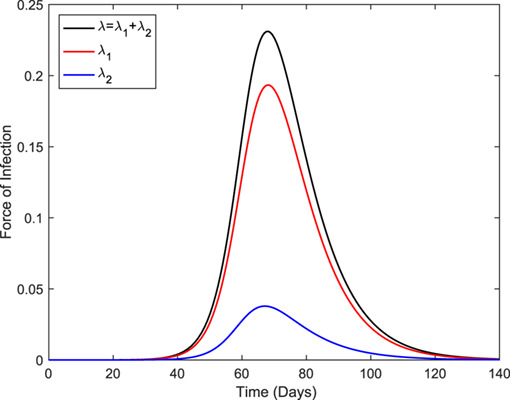
The forces of infection  (young subpopulation),
  (elder subpopulation), and
  (entire population).
The peaks of the force of infection for  ,
,  and
and  are, respectively,
  ,
,  , and
, and  , which occur at the simulation times
  ,
,  , and
, and  (days), and the contributions of
  and
and  with respect to
  are
are  and
and  . The ratio between peaks
  :
: is
is  :
: , which is close to the ratio between the numbers of young:elder
  :
: . When the virus circulates in mixed subpopulations, young and elder persons are infected additionally by, respectively, elder (
 ) and young (
 ) persons. This fact is the reason for the actual equilibrium values being bigger (
 and
and  ), but among elder persons, the increase (
 times) is enormous (
 , relatively big, acts on relatively small population
  ). For this reason, contacts between elder and young persons must be avoided.
Finally, let us discriminate the circulation of the new coronavirus in a community without any control. Figure 25 shows all persons harboring this virus ( ,
,  ,
,  ,
,  and
and  ), for young (a) and elder (b) subpopulations. Notice that the exposed (
 ) and pre-diseased (
 ) persons are relatively higher in the young subpopulation.
Fig. 25.
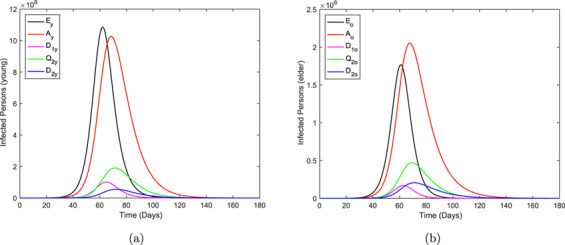
The curves of all persons harboring the new coronavirus ( ,
,  ,
,  ,
,  and
and  ),
),  , for the young and elder subpopulations.
In Fig. 26, we show the ratio hidden:apparent based on Fig. 25. Those who harbor the new coronavirus as exposed and those who do not manifest symptoms are classified in the hidden category, and in the apparent category, we include those who manifest symptoms. Hence the ratio is calculated as  . At
. At  , the ratio is
  for young and elder persons due to initial conditions.
Fig. 26.
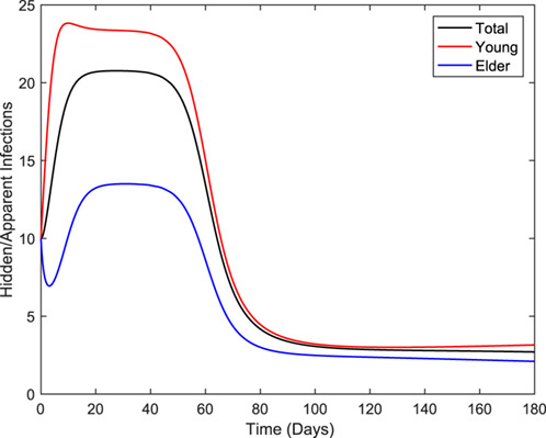
The curves of the ratio hidden:apparent for young, elder and total persons.
Comparing Figs 25 and 26, as the epidemic evolves, the ratio increases quickly at the beginning, reaches a plateau during the increasing phase and decreases quickly during the declining phase, and finally reaches another plateau after the ending phase of the first wave. In the first plateau, the ratios are 14:1, 23:1 and 21:1 for, respectively, elder, young and entire persons. The second plateau (3:1) is reached when the first wave of the epidemic is ending. Therefore, there are much more hidden than apparent persons during the epidemic, which indicates that the control of CoViD-19 by isolation must be accompanied by mass testing to find infected persons.
5. Conclusion
We formulated a mathematical model considering two subpopulations comppsed of young and elder subpopulations to study CoViD-19 in São Paulo State, Brazil. The model considered continuous but constant rates of isolation and relaxation. We change the rates describing the isolation and release by proportions of susceptible persons being isolated or released in future work.4 The reason behind this is the difficulty of establishing a relationship between rates and proportions.
Our model estimated quite the same number of severe CoViD-19 cases predicted by Ferguson et al. (2020) for Brazil, as well as the number of deaths due to CoViD-19. However, the second estimation method provided  times lower for fatalities due to CoViD-19, hence the difference relays mainly in the estimation method for the additional mortality rates.5
Suppose the currently adopted lockdown is indeed based on the goal of decreasing hospitalized CoViD-19 cases. In that case, our model agrees since it predicts that a higher number of young and elder persons must be isolated to achieve this objective. However, if the goal is to reduce the number of deaths due to CoViD-19, elder persons must be isolated in a higher number than young persons. Remember that in mixed young and elder subpopulations, the infection is much harmful in the elder than in young persons, which is a reason to avoid contact between them. Optimal rates of isolation in young and elder subpopulations to reduce both CoViD-19 cases and deaths can be obtained by optimal control theory (Thomé et al., 2009).
If vaccine and efficient treatments are available, the new coronavirus epidemic should not be considered a threat to public health. However, currently, there is no vaccine neither efficient treatment.6 For this reason, the adoption of the isolation or lockdown is the best-recommended strategy, which can be less hardly implemented if there is enough kit to test against the new coronavirus. Remember that all isolation strategies considered in our model assumed the identification of the susceptible persons. Finally, the isolation as a control mechanism delayed the peak of the epidemic, which may avoid the overloading in hospitals and ICUs, besides providing an additional time to seek a cure (medicine) and or development of a vaccine.
Acknowledgements
We thank the anonymous referee for providing comments and suggestions, which contributed to improving this paper.
Financial support
This research received no specific grant from any funding agency, commercial or not-for-profit sectors.
Declaration of interest
Declarations of interest: None.
A. The trivial equilibrium point and its stability
By the fact that  is varying, the system of equations (2), (3) and (4) in the main text is non-autonomous non-linear differential equations. To obtain an autonomous system of equations, we use the fractions of individuals in each compartment, defined by, with
  and
and  ,
,
 |
resulting in
 |
using equation (5) for  . Hence, equations (2), (3) and (4) in terms of the fractions become autonomous non-linear system of equations, with equations for susceptible persons,
 |
(A.1) |
for susceptible persons in isolation  and for infected persons,
 |
(A.2) |
and for immune persons,
 |
(A.3) |
where  is the force of infection given by equation (1) re-written as
 |
and
 |
We remember that all classes vary with time; however, their fractions attain a steady-state (the sum of all classes’ derivatives is zero). This system of equations is not easy to determine the non-trivial (endemic) equilibrium point  . Hence, we restrict our analysis to the trivial (disease-free) equilibrium point.
The trivial or disease-free equilibrium point  is given by
 |
for  and
and  , where
 |
(A.4) |
with  .
.
Due to the high number of equations, we do not deal with characteristic equation corresponding to the Jacobian matrix evaluated at  , but we apply the next-generation matrix theory (Diekmann et al., 2010). The next-generation matrix, evaluated at the trivial equilibrium point
  , is obtained considering the vector of variables
  . Instead of calculating the spectral radius corresponding to the next generation matrix, we apply the method proposed in Yang (2014) and proved in Yang (2017). Notice that control mechanisms are considered, hence we are obtaining the reduced reproduction number
  .
.
A.1 Local stability of 
The next generation matrix is constructed considering a subsystem of equations (2), (3) and (4) taking into account the state-at-infection ( ) and the states-of-infectiousness (
 ,
, ) (Diekmann et al., 2010), resulting in
  . In a matrix form, the subsystem is written as
 |
where the vectors  and
and  are defined below, with the partial derivatives of
  and
and  evaluated at
  being given by
 |
(A.5) |
Depending on the choice of vectors  and
and  , we can obtain the reduced reproduction number or the fraction of susceptible persons at endemic level (Yang, 2014).
A.1.1 The reduced reproduction number
In order to obtain the reduced reproduction number  , diagonal matrix
  is considered (Yang, 2014). Hence, the vectors
  and
and  are
are
 |
(A.6) |
and
 |
(A.7) |
where the superscript  stands for the transposition of a matrix, from which we obtain the matrices
  and
and  using equation (A.5) evaluated at the trivial equilibrium
  . The matrix
  is given by
 |
(A.8) |
and the matrix  is given by
 |
(A.9) |
where  and
and  . The next generation matrix
  is, then,
 |
and the characteristic equation corresponding to  , obtained from
  , with
  being the
  identity matrix, is
 |
(A.10) |
where the reduced reproduction number  is
is
 |
(A.11) |
and  and
and  are the partial reproduction numbers defined by
 |
(A.12) |
Instead of calculating the spectral radius ( ) of the characteristic equation (A.10), we apply procedure in Yang (2014) (the sum of coefficients of characteristic equation), resulting in the threshold
  . Hence, the trivial equilibrium point
  is locally asymptotically stable (LAS) if
  .
.
When a protection mechanism is introduced in a population, the basic reproduction number  is decreased to
  , the reduced reproduction number. The safety of susceptible persons is done by a vaccine (not yet available) or isolation (or quarantine). The isolation was described by the isolation rate of susceptible persons
  , with
  . When
  , the fraction of young persons and elders are, from equation (A.4),
 |
(A.13) |
with  . The basic reproduction number
  is retrieved letting
  , with
  , in equation (A.12), resulting in
 |
(A.14) |
with  and
and  being the partial reproduction numbers given by
 |
The partial reproduction number  (or
(or  ) is the secondary cases produced by one case of asymptomatic individual (or pre-diseased individual) in a completely susceptible young subpopulation without control. The partial basic reproduction number
  (or
(or  ) is the secondary cases produced by one case of asymptomatic individual (or pre-diseased individual) in a completely susceptible elder subpopulation without control. If all parameters are equal, and
  , then
 |
where  and
and  are the partial reproduction numbers due to the asymptomatic and pre-diseased persons.
A.1.2 The fraction of susceptible persons
To obtain the fraction of susceptible individuals,  must be the most straightforward (matrix with the least number of non-zero elements) (Yang, 2014). Hence, the vectors
  and
and  are
are
 |
and
 |
from which we obtain the matrices  and
and  using equation (A.5) evaluated at the trivial equilibrium
  . The matrix
  is given by
 |
and the matrix  is given by
 |
where  and
and  . The next generation matrix
  is
is
 |
and the characteristic equation corresponding to  is
is
 |
The spectral radius is  given by equation (A.11). Hence, the trivial equilibrium point
  is LAS if
  .
.
Both procedures resulted in the same threshold, hence, according to Yang & Greenhalgh (2015), the inverse of the reduced reproduction number  given by equation (A.11) is a function of the fraction of susceptible individuals at endemic equilibrium
  through
 |
(A.15) |
where  (see Yang et al., 2016; Yang & Greenhalgh, 2015). For this reason, the effective reproduction number
  (Yang, 2020), which varies with time, cannot be defined by
  , or
, or  . The function
  is determined by calculating the coordinates of the non-trivial equilibrium point
  . For instance, for dengue transmission model,
  , where
  and
and  are the fractions at equilibrium of, respectively, humans and mosquitoes (Yang et al., 2016). For tuberculosis model considering drug-sensitive and resistant strains, there is not
  , but
, but  is solution of a second degree polynomial (Yang & Greenhalgh, 2015).
From equation (A.15), let us use as an approximation that  . Then, we can define the effective reproduction number
  as
as
 |
(A.16) |
which depends on time, and when attains steady state ( ), we have
  .
.
A.2 Global stability of 
The global stability of  follows the method proposed in Shuai & Driessche (2013). Let the vector of variables be
  , vectors
  and
and  given by equations (A.6) and (A.7) and matrices
  and
and  given by equations (A.8) and (A.9). The vector
  , constructed as
 |
is
 |
where  if
if  ,
,  and
and  .
.
Let  be the left eigenvector satisfying the equation
  , where
  is the spectral radius of the characteristic equation (A.10), and
 |
We must solve the system of equations
 |
and the vector-solution is given by
 |
A Lyapunov function  can be constructed as
  , resulting in
 |
which is always positive or zero ( ), and
 |
which is negative or zero ( ) only if
  ,
,  ,
,  and
and  (conditions to have
  ).
).
Hence, the method proposed in Shuai & Driessche (2013) is valid only for  , in which case
  is globally stable if
  ,
,  and
and  .
.
Footnotes
Simulations were done on April 6.
On April 6 the isolation was extended until April 22.
Simulations were done on April 10.
The model proposed here can easily be modified to consider the Dirac delta function to describe the isolation and releases, i.e. isolation and releases are supplied to the dynamical system as pulses. For instance, the isolation can be introduced in the model changing  by
by  , where
  is the proportion in isolation,
  is the time at which isolation was implemented, and
  is the Dirac delta function. The model presented here and the modified model using the Dirac function estimate well the transmission rates and parameters related to isolation when incorporating more observed data.
If we use the fact that the time of registration  of deaths
  must be related to the deaths of new cases
  times ago, i.e.
  , then the observed accumulated number of deaths due to CoViD-19 is nicely fitted, and its fitting at the ending phase of the epidemic is quite similar than that provided by the second method.
Additional protective measures adopted by the population are the use of a face mask, washing hands with alcohol and gel, and social distancing. This kind of control aiming at the reduction in the transmission can be incorporated in the model introducing a reduction parameter  in the force of the infection, i.e. changing
  by
by  , with
  .
.
References
- Anderson, R. M. & May, R. M. (1991) Infectious Diseases of Human. Dynamics and Control. Oxford, New York, Tokyo: Oxford University Press. [Google Scholar]
- Boletim Epidemiológico 08 (2020), https://www.saude.gov.br/images/pdf/2020/April/09/be-covid-08-final-2.pdf.
- Diekmann, O., Heesterbeek, J. A. P. & Roberts, M. G. (2010) The construction of next-generation matrices for compartmental epidemic models. J. R. Soc. Interface, 7, 873–885. [DOI] [PMC free article] [PubMed] [Google Scholar]
- Ferguson, N. M., et al. (2020) Impact of Non-Pharmaceutical Interventions (NPIs) to Reduce COVID-19 Mortality and Healthcare Demand. Imperial College COVID-19 Response Team. [DOI] [PMC free article] [PubMed] [Google Scholar]
- Li, R.Y., et al. . (2020) Substantial undocumented infection facilitates the rapid dissemination of novel coronavirus (SARS-CoV2). Science, eabb3221. [DOI] [PMC free article] [PubMed]
- Raimundo, S. M., Yang, H. M., Bassanezi, R. C. & Ferreira, M. A. C. (2002) The attracting basins and the assessment of the transmission coefficients for HIV and M. tuberculosis infections among women inmates. J. Biol. Syst., 10, 61–83. [Google Scholar]
- SEADE–Fundação Sistema Estadual (2020) https://www.seade.gov.br.
- Shuai, Z. & van den Driessche, P. (2013) Global stability of infectious disease model using Lyapunov functions. SIAM J. Appl. Math., 73, 1513–1532. [Google Scholar]
- Thomé, R. C. A., Yang, H. M. & Eesteva, L. (2009) Optimal control of Aedes aegypti mosquitoes by the sterile insect eechnique and insecticide. Math. Biosci., 223, 12–23. [DOI] [PubMed] [Google Scholar]
- WHO (2020) Report of the WHO-China Joint Mission on Coronavirus Disease 2019 (COVID-19), 16–24 February 2020.
- Yang, H. M. (1998) Modelling vaccination strategy against directly transmitted diseases using a series of pulses. J. Biol. Syst., 6, 187–212. [Google Scholar]
- Yang, H. M. (1999a) Directly transmitted infections modeling considering age-structured contact rate—epidemiological analysis. Math. Comput. Model., 29, 11–30. [Google Scholar]
- Yang, H. M. (1999b) Directly transmitted infections modeling considering age-structured contact rate. Math. Comput. Model., 29, 39–48. [Google Scholar]
- Yang, H. M. (2001) Modeling directly transmitted infections in a routinely caccinated population—the force of infection described by Volterra integral equation. Appl. Math. Comput., 122, 27–58. [Google Scholar]
- Yang, H. M. (2014) The basic reproduction number obtained from Jacobian and next generation matrices—a case study of dengue transmission modelling. BioSystems, 126, 52–75. [DOI] [PubMed] [Google Scholar]
- Yang, H. M. (2017) The transovarial transmission un the dynamics of dengue infection: epidemiological implications and thresholds. Math. Biosc., 286, 1–15. [DOI] [PubMed] [Google Scholar]
- Yang, H. M. (2020) Are the beginning and ending phases of epidemics provided by next generation matrices?—Revisiting drug sensitive and resistant tuberculosis model. J. Biol. Syst. (in press). [Google Scholar]
- Yang, H. M., Boldrini, J. L., Fassoni, A. C., Lima, K. K. B., Freitas, L. S. F., Gomez, M. C., Andrade, V. F. & Freitas, A. R. R. (2016) Fitting the incidence data from the City of Campinas, Brazil, based on dengue transmission modellings considering time-dependent entomological parameters. PLoS One, 11, 1–41. [DOI] [PMC free article] [PubMed] [Google Scholar]
- Yang, H. M. & Greenhalgh, D. (2015) Proof of conjecture in: the basic reproduction number obtained from Jacobian and next generation matrices—a case study of dengue transmission modelling. Appl. Math. Comput., 265, 103–107. [DOI] [PubMed] [Google Scholar]