Mathematical analysis and simulation of a stochastic COVID-19 Lévy jump model with isolation strategy

Abstract

This paper investigates the dynamics of a COVID-19 stochastic model with isolation strategy. The white noise as well as the Lévy jump perturbations are incorporated in all compartments of the suggested model. First, the existence and uniqueness of a global positive solution are proven. Next, the stochastic dynamic properties of the stochastic solution around the deterministic model equilibria are investigated. Finally, the theoretical results are reinforced by some numerical simulations.

Introduction

Infectious diseases modeling has captivated the interest of many research works during the last recent years [1], [6], [2], [3], [4], [5], [7]. The basic SIR model representing the dynamics behavior of the three main populations that represent the susceptible $\left(S\right)$, the infected $\left(I\right)$ and the recovered $\left(R\right)$, was firstly proposed in 1927 by Kermack and Mc Kendricks [8]; the suggested model has played an important role in starting different research works in disease dynamics field. Understanding the interaction dynamics between the different infection components becomes then an important issue to prevent many serious infectious disease outbreaks. For instance, several mathematical models have been used to better understand the behavior of various viral infections, such as the hepatitis B virus (HBV) [6], [10], [9], [11], [12] human immunodeficiency virus (HIV) [1], [14], [2], [13], [15], [3], [4] or hepatitis C virus (HCV) [16], [19], [18], [17].

COVID-19 is a recent pandemic disease that was behind a great disaster worldwide. Since there is still no efficient vaccine against COVID-19, substantial number of researches are undertaken in order to understand the disease mechanism, reduce the disease spread and find some solutions to this serious infection. As it was established, COVID-19 is the recent form of coronavirus infection induced by the already known severe acute respiratory syndrome SARS-CoV-2 [20], [21], [22], [23]. This recently discovered disease can be transmitted from an infected to any close unprotected person; likewise the susceptible can become an infected individual when touching any contaminated area [24]. Hence, isolating infected persons from the other susceptible population becomes more and more an important mean to reduce and overcome COVID-19 propagation.

Recently, different models have been investigated to study COVID-19. For instance, the risk estimation, the infection evolution and the prediction of COVD-19 infection is studied [25], [26], [27], [28]; the authors concludes that for ensuring a quick ending of the epidemic, the interventions strategy and self-protection measures should always be maintained. The meteorological role and policy measures on COVD-19 spread were studied in [29], [30]; it was concluded that the policy strategy has reduced the infection and the meteorological role can be considered as an important factor in controlling COVID-19. The effect of quarantine on coronavirus was discussed in [31]; the results confirm the importance of reducing contact between the infected and other individuals.

Since the isolation strategy is an important tool to reduce the infection, adding another component representing the isolated individuals $\left(\mathcal{Q}\right)$ to the classical SIR model becomes primordial; and the new epidemiological model will be under SIQR abbreviation [32].

To investigate the dynamics of COVID-19 in this paper, we subdivide the total population into four different epidemiological classes in which their descriptions are defined later. The parameters used in the co-infection model are summarized in Table 1, Table 2 , and the schematic diagram of the compartmental COVID model is shown in Fig. 1 .

Table 1.

The sensitivity indices of $R_0$.

Parameters	Sensitivity index
$\lambda$	1
$\beta$	1
$\zeta$	$-2.39$
$\upsilon$	$0.921$
$\kappa$	$0.514$
d	$0.334$

Table 2.

The used parameters for the numerical simulations.

Parameters	Fig. 2	Fig. 3	references
$\lambda$	$1785.205$	$1785.205$	[43]
$\zeta$	$0.35$	$0.49$	–
$\beta$	$0.13$	$0.13$	[43]
$\upsilon$	$2.7\times {10}^{-4}$	$0.03$	–
$\kappa$	$0.15$	$0.35$	[43]
d	$0.038$	$0.038$	[43]
${\sigma }_1$	${10}^{-4}$	${10}^{-5}$	–
${\sigma }_2$	$2\times {10}^{-4}$	$2\times {10}^{-4}$	–
${\sigma }_3$	$2\times {10}^{-4}$	$2\times {10}^{-3}$	–
${\sigma }_4$	$2\times {10}^{-4}$	$2\times {10}^{-4}$	–
${\mathcal{q}}_1\left(u\right)$	$-0.04$	$-0.04$	–
${\mathcal{q}}_2\left(u\right)$	$-0.006$	$-0.006$	–
${\mathcal{q}}_3\left(u\right)$	$-0.008$	$-0.008$	–
${\mathcal{q}}_4\left(u\right)$	$-0.009$	$0.009$	–

Fig. 1.

The transfer diagram for the SIQR model.

The SIQR deterministic system of equations may take the following form:

$$\left\{\begin{array}{cc}\frac{d\mathcal{S}}{\mathit{dt}}\left(t\right)=\hfill & \lambda -\zeta \mathcal{S}\left(t\right)-\beta \mathcal{S}\left(t\right)\mathcal{I}\left(t\right),\hfill \\ \hfill \\ \frac{d\mathcal{I}}{\mathit{dt}}\left(t\right)=\hfill & \beta \mathcal{S}\left(t\right)\mathcal{I}\left(t\right)-(\zeta +\upsilon )\mathcal{I}\left(t\right),\hfill \\ \hfill \\ \frac{d\mathcal{Q}}{\mathit{dt}}\left(t\right)=\hfill & \upsilon \mathcal{I}\left(t\right)-(\zeta +\kappa +d)\mathcal{Q}\left(t\right),\hfill \\ \hfill \\ \frac{d\mathcal{R}}{\mathit{dt}}\left(t\right)=\hfill & \kappa \mathcal{Q}\left(t\right)-\zeta \mathcal{R}\left(t\right),\hfill \end{array}\right)$$ (1)

where $\lambda$ is the birth average of the susceptibles, their mortality rate is denoted by $\zeta \mathcal{S}$. The susceptible become infected at a rate $\beta \mathcal{SI}$, the death rate of infected population is denoted by $\zeta \mathcal{I}$; the infected become isolated at rate $\upsilon \mathcal{I}$. The death rate of the isolated individuals due to the infection is represented $d\mathcal{Q}$ and due to others means is $\zeta \mathcal{Q}$. Finally, the isolated become recovered at rate $\kappa \mathcal{Q}$; the death rate of the recovered is denoted by $\zeta \mathcal{R}$.

On the hand, stochastic quantification of several real life phenomena have been much helpful in understanding the random nature of their incidence or occurrence. This also helped in finding solutions to such problems arising from them either in form of minimization of their undesirability or maximizing their rewards. Besides, the infectious diseases are exposed to randomness and uncertainty in terms of normal infection progress. Therefore, the stochastic modeling are more appropriate comparing to the deterministic models; considering the fact that the stochastic systems do not take into account only the variable mean but also the standard deviation behavior surround it. Moreover, the deterministic systems generate similar results for initial fixed values, but the stochastic ones can give different predicted results. Several stochastic infectious models describe the effect of white noise on viral dynamics have been deployed [33], [7], [34]. Recently and in the same context, a stochastic SIQR model is studied in [35], the authors introduce the Brownian perturbation to the four components of the model and study the different conditions of extinction and persistence of the infection. Both of white and telegraph noises were taken into consideration to study SIQR model [36], sufficient different conditions to establish persistence in mean were studied.

In addition to the cited random noises, Lévy jumps present an important tool to model many real dynamical phenomena [37], [38]. Indeed, because of the unpredictable stochastic properties of the disease progression, infection dynamical model may know sudden significant perturbations in the disease process [39]. Then, it will be more reasonable to illustrate those sudden fluctuations through an introduction of the Lévy jump behavior into the infection model. For instance, Berrhazi et al. [40] studied, recently, a stochastic SIRS model under Lévy jumps fluctuations and considering bilinear function describing the infection. The uniqueness of global solution was established, also through suitable Lyapunov functions, it was demonstrated that the stochastic stability of steady states depends on some sufficient conditions for persistence or extinction of the studied infection. Motivated by the previous works, we will consider in this paper the following stochastic SIQR model driven by Lévy noise:

$$\left\{\begin{array}{cc}d\mathcal{S}\left(t\right)=\hfill & \left(\lambda -\zeta \mathcal{S}\left(t\right)-\beta \mathcal{S}\left(t\right)\mathcal{I}\left(t\right)\right)\mathit{dt}+{\sigma }_1\mathcal{S}\left(t\right){\mathit{dW}}_1\left(t\right)+{\int }_U{\mathcal{q}}_1\left(u\right)\mathcal{S}(t-)\tilde{N}(\mathit{dt},\mathit{du}),\hfill \\ d\mathcal{I}\left(t\right)=\hfill & \left(\beta \mathcal{S}\left(t\right)\mathcal{I}\left(t\right)-(\zeta +\upsilon )\mathcal{I}\left(t\right)\right)\mathit{dt}+{\sigma }_2\mathcal{I}\left(t\right){\mathit{dW}}_2\left(t\right)+{\int }_U{\mathcal{q}}_2\left(u\right)\mathcal{I}(t-)\tilde{N}(\mathit{dt},\mathit{du}),\hfill \\ d\mathcal{Q}\left(t\right)=\hfill & \left(\upsilon \mathcal{I}\left(t\right)-(\zeta +\kappa +d)\mathcal{Q}\left(t\right)\right)\mathit{dt}+{\sigma }_3\mathcal{Q}\left(t\right){\mathit{dW}}_3\left(t\right)+{\int }_U{\mathcal{q}}_3\left(u\right)\mathcal{Q}(t-)\tilde{N}(\mathit{dt},\mathit{du}),\hfill \\ d\mathcal{R}\left(t\right)=\hfill & \left(\kappa \mathcal{Q}\left(t\right)-\zeta \mathcal{R}\left(t\right)\right)\mathit{dt}+{\sigma }_4\mathcal{R}\left(t\right){\mathit{dW}}_4\left(t\right)+{\int }_U{\mathcal{q}}_4\left(u\right)\mathcal{R}(t-)\tilde{N}(\mathit{dt},\mathit{du}),\hfill \end{array}\right)$$ (2)

where $W_i\left(t\right)$ is a standard Brownian motion defined on a complete probability space $\left(\mathrm{\Omega },\mathcal{F},{\left({\mathcal{F}}_t\right)}_{t⩾0},\mathbb{P}\right)$ with the filtration ${\left({\mathcal{F}}_t\right)}_{t⩾0}$ satisfying the usual conditions. We denote by $\mathcal{S}(t-),\mathcal{I}(t-)$ , $\mathcal{Q}(t-)$ and $\mathcal{R}(t-)$ the left limits of $\mathcal{S}\left(t\right),\mathcal{I}\left(t\right),\mathcal{Q}\left(t\right)$ and $\mathcal{R}\left(t\right)$ respectively. $N(\mathit{dt},\mathit{du})$ is a Poisson counting measure with the stationary compensator $\nu \left(\mathit{du}\right)\mathit{dt},\tilde{N}(\mathit{dt},\mathit{du})=N(\mathit{dt},\mathit{du})-\nu \left(\mathit{du}\right)\mathit{dt}$ with $\nu \left(U\right)<\infty$ and ${\sigma }_i$ is the intensity of $W_i\left(t\right)$. The jumps intensities are represented by ${\mathcal{q}}_i\left(u\right)$ with $i=1,\dots ,4$.

The present work will be organized as follows. The next section is devoted to establish the existence and uniqueness of the global positive solution to the studied model (2). We calculate the basic reproduction number and the different problem equilibria in Section “The basic reproduction number and equilibria”. The stochastic behavior of the solution of the disease-free equilibrium is studied in Section “The stochastic property around the free-infection equilibrium”. The dynamics of the solution of the endemic equilibrium is studied in Section “The stochastic property around the endemic equilibrium”. The sensitivity analysis is presented in Section “Sensitivity analysis”. The final part of this paper is dedicated to some numerical results in order to support the theoretical findings.

The existence and uniqueness of global positive solution

The existence and uniqueness of the problem (2) global positive solution is guaranteed by the next following theorem.

Theorem 1

For any initial condition in${\mathbb{R}}_{+}^4$, the model(2)has a unique global solution$\left(\mathcal{S}\left(t\right),\mathcal{I}\left(t\right),\mathcal{Q}\left(t\right),\mathcal{R}\left(t\right)\right)\in {\mathbb{R}}_{+}^4$almost surely.

Proof

First, we know that the diffusion and the drift are locally Lipschitz functions, therefore for any initial condition $\left(\mathcal{S}\left(0\right),\mathcal{I}\left(0\right),\mathcal{Q}\left(0\right),\mathcal{R}\left(0\right)\right)\in {\mathbb{R}}_{+}^4$, we have the existence of a unique local solution $\left(\mathcal{S}\left(t\right),\mathcal{I}\left(t\right),\mathcal{Q}\left(t\right),\mathcal{R}\left(t\right)\right)$ for $t\in [0,t_e)$, where $t_e$ is the time of explosion.

In order to demonstrate that this solution is globally defined, we need to check that $t_e=\infty$ a.s. Firstly, we will demonstrate that $\left(\mathcal{S}\left(t\right),\mathcal{I}\left(t\right),\mathcal{Q}\left(t\right),\mathcal{R}\left(t\right)\right)$ do not tend to infinity for a bounded time. Let $m_0>0$, be sufficiently a large number, in such manner that $\left(\mathcal{S}\left(0\right),\mathcal{I}\left(0\right),\mathcal{Q}\left(0\right),\mathcal{R}\left(0\right)\right)$ be within the interval $[\frac{1}{m_0},m_0]$. We define, for each integer $m⩾m_0$, the stopping time

$$t_m=\inf \{t\in [0,t_e)/\mathcal{S}(t)\notin (\frac{1}{m},m\left)\mathrm{or}\mathcal{I}\right(t)\notin (\frac{1}{m},m\left)\mathrm{or}\mathcal{Q}\right(t)\notin (\frac{1}{m},m\left)\mathrm{or}\mathcal{R}\right(t)\notin (\frac{1}{m},m\left)\right\},$$

where $t_m$ is an increasing number when $m\uparrow \infty$. Let $t_{\infty }={\lim }_{m\to \infty }{t}_m$, where $t_{\infty }⩽t_e$ a.s. We need to show that $t_{\infty }=\infty$ which means that $t_e=\infty$ and $\left(\mathcal{S}\left(t\right),\mathcal{I}\left(t\right),\mathcal{Q}\left(t\right),\mathcal{R}\left(t\right)\right)\in {\mathbb{R}}_{+}^4$ a.s. Assume the opposite case is verified, i.e. $t_{\infty }<\infty$ a.s. Therefore, there exist two constants $0<∊<1$ and $T>0$ such that $\mathbb{P}(t_{\infty }⩽T)⩾∊$.

Therefore, there exists an integer $m_1⩾m_0$ such that $\mathbb{P}(t_m⩽T)⩾∊\mathrm{forall}m⩾m_1$.

Let’s now consider the following functional

$$\begin{array}{c}\hfill \mathcal{V}\left(\mathcal{S}\left(t\right),\mathcal{I}\left(t\right),\mathcal{Q}\left(t\right),\mathcal{R}\left(t\right)\right)=\left(\mathcal{S}-a-a\log \left(\frac{\mathcal{S}}{a}\right)\right)+\left(,\mathcal{I}-1-\log \left(,\mathcal{I}\right)\right)\\ \hfill +\left(\mathcal{Q}-1-\log \left(\mathcal{Q}\right)\right)+\left(\mathcal{R}-1-\log \left(\mathcal{R}\right)\right),\end{array}$$

with a is a positive constant.

Let $m⩾m_0$ and $T>0$ be arbitrary. For any $0⩽t⩽t_m\wedge T=\mathit{min}(t_m,T)$. From Itô’s formula, we will have

$$\begin{array}{cc}d\mathcal{V}\left(\mathcal{S},\mathcal{I},\mathcal{Q},\mathcal{R}\right)=\hfill & \mathit{LV}\mathit{dt}+{\sigma }_1(\mathcal{S}-a){\mathit{dW}}_1+{\sigma }_2(\mathcal{I}-1){\mathit{dW}}_2+{\sigma }_3(\mathcal{Q}-1){\mathit{dW}}_3+{\sigma }_4(\mathcal{R}-1){\mathit{dW}}_4\hfill \\ \hfill & +{\int }_U\left[{\mathcal{q}}_1\left(u\right)\mathcal{S}-a\log \left(1+{\mathcal{q}}_1\left(u\right)\right)\right]\tilde{N}(\mathit{dt},\mathit{du})\hfill \\ \hfill & +{\int }_U\left[{\mathcal{q}}_2\left(u\right)\mathcal{I}-\log \left(1+{\mathcal{q}}_2\left(u\right)\right)\right]\tilde{N}(\mathit{dt},\mathit{du})\hfill \\ \hfill & +{\int }_U\left[{\mathcal{q}}_3\left(u\right)\mathcal{Q}-\log \left(1+{\mathcal{q}}_3\left(u\right)\right)\right]\tilde{N}(\mathit{dt},\mathit{du})\hfill \\ \hfill & +{\int }_U\left[{\mathcal{q}}_4\left(u\right)\mathcal{R}-\log \left(1+{\mathcal{q}}_4\left(u\right)\right)\right]\tilde{N}(\mathit{dt},\mathit{du}),\hfill \end{array}$$ (3)

where

$$\begin{array}{c}\hfill L\mathcal{V}=\left(1-\frac{a}{\mathcal{S}}\right)\left(\lambda -\zeta \mathcal{S}\left(t\right)-\beta \mathcal{S}\left(t\right)\mathcal{I}\left(t\right)\right)+\frac{a{\sigma }_1^2}{2}\\ \hfill +\left(1-\frac{1}{\mathcal{I}}\right)\left(\beta \mathcal{S}\left(t\right)\mathcal{I}\left(t\right)-(\zeta +\upsilon )\mathcal{I}\left(t\right)\right)+\frac{{\sigma }_2^2}{2}\\ \hfill +\left(1-\frac{1}{\mathcal{Q}}\right)\left(\upsilon \mathcal{I}\left(t\right)-(\zeta +\kappa )\mathcal{Q}\left(t\right)\right)+\frac{{\sigma }_3^2}{2}\\ \hfill +\left(1-\frac{1}{\mathcal{R}}\right)\left(\kappa \mathcal{Q}\left(t\right)-\zeta \mathcal{R}\right)+\frac{{\sigma }_4^2}{2}\\ \hfill +{\int }_U\left[{\mathcal{q}}_1\left(u\right)-\log \left(1+{\mathcal{q}}_1\left(u\right)\right)\right]\nu \left(\mathit{du}\right)\\ \hfill +{\int }_U\left[{\mathcal{q}}_2\left(u\right)-\log \left(1+{\mathcal{q}}_2\left(u\right)\right)\right]\nu \left(\mathit{du}\right)\\ \hfill +{\int }_U\left[{\mathcal{q}}_3\left(u\right)-\log \left(1+{\mathcal{q}}_3\left(u\right)\right)\right]\nu \left(\mathit{du}\right)\\ \hfill +{\int }_U\left[{\mathcal{q}}_4\left(u\right)-\log \left(1+{\mathcal{q}}_4\left(u\right)\right)\right]\nu \left(\mathit{du}\right),\end{array}$$

therefore, we will have

$$\begin{array}{c}\hfill L\mathcal{V}⩽\lambda +\zeta +a\zeta +\left(a\beta -\zeta \right)\mathcal{I}+\left(\zeta +\upsilon \right)+(\zeta +\kappa )\\ \hfill +\frac{a{\sigma }_1^2}{2}+\frac{{\sigma }_2^2}{2}+\frac{{\sigma }_3^2}{2}+\frac{{\sigma }_4^2}{2}\\ \hfill +{\int }_U\left(a{\mathcal{q}}_1\left(u\right)-a\log \left(1+{\mathcal{q}}_1\left(u\right)\right)\right)\nu \left(\mathit{du}\right)\\ \hfill +{\int }_U\left({\mathcal{q}}_2\left(u\right)-\log \left(1+{\mathcal{q}}_2\left(u\right)\right)\right)\nu \left(\mathit{du}\right)\\ \hfill +{\int }_U\left({\mathcal{q}}_3\left(u\right)-\log \left(1+{\mathcal{q}}_3\left(u\right)\right)\right)\nu \left(\mathit{du}\right)\\ \hfill +{\int }_U\left({\mathcal{q}}_4\left(u\right)-\log \left(1+{\mathcal{q}}_4\left(u\right)\right)\right)\nu \left(\mathit{du}\right),\end{array}$$

by choosing $a=\frac{\zeta }{\beta }$, we will get

$$\begin{array}{c}\hfill L\mathcal{V}⩽\lambda +\zeta +\frac{{\zeta }^2}{\beta }+\left(\zeta +\upsilon \right)+(\zeta +\kappa )\\ \hfill +\frac{\zeta {\sigma }_1^2}{2\beta }+\frac{{\sigma }_2^2}{2}+\frac{{\sigma }_3^2}{2}+4M\prime =M,\end{array}$$

where

$$\begin{array}{c}\hfill M\prime =\max \left\{{\int }_U\frac{\zeta }{\beta }\left({\mathcal{q}}_1\left(u\right)-\log \left(1+{\mathcal{q}}_1\left(u\right)\right)\right)\nu \left(\mathit{du}\right),{\int }_U\left({\mathcal{q}}_2\left(u\right)-\log \left(1+{\mathcal{q}}_2\left(u\right)\right)\right)\nu \left(\mathit{du}\right),\right)\\ \hfill \left({\int }_U\left({\mathcal{q}}_3\left(u\right)-\log \left(1+{\mathcal{q}}_3\left(u\right)\right)\right)\nu \left(\mathit{du}\right),{\int }_U\left({\mathcal{q}}_4\left(u\right)-\log \left(1+{\mathcal{q}}_4\left(u\right)\right)\right)\nu \left(\mathit{du}\right)\right\}\text{.}\end{array}$$

Integrating both sides of the Eq. (3) between 0 and $t_m\wedge T$, we get

$$\begin{array}{c}\hfill {\int }_0^{t_m\wedge T}d\mathcal{V}\left(\mathcal{S}\left(t\right),\mathcal{I}\left(t\right),\mathcal{Q}\left(t\right),\mathcal{R}\left(t\right)\right)\mathit{dt}⩽{\int }_0^{t_m\wedge T}M\mathit{dt}+{\sigma }_1{\int }_0^{t_m\wedge T}(\mathcal{S}-\frac{\zeta }{\beta }){\mathit{dW}}_1\left(t\right)+{\sigma }_2{\int }_0^{t_m\wedge T}(\mathcal{I}-1){\mathit{dW}}_2\left(t\right)\\ \hfill +{\sigma }_3{\int }_0^{t_m\wedge T}(\mathcal{Q}-1){\mathit{dW}}_3\left(t\right)+{\sigma }_4{\int }_0^{t_m\wedge T}(\mathcal{R}-1){\mathit{dW}}_4\left(t\right)\\ \hfill +{\int }_0^{t_m\wedge T}{\int }_U\left[{\mathcal{q}}_1\left(u\right)\mathcal{S}-\frac{\zeta }{\beta }\log \left(1+{\mathcal{q}}_1\left(u\right)\right)\right]\tilde{N}(\mathit{dt},\mathit{du})\mathit{dt}\\ \hfill +{\int }_0^{t_m\wedge T}{\int }_U\left[{\mathcal{q}}_2\left(u\right)\mathcal{I}-\log \left(1+{\mathcal{q}}_2\left(u\right)\right)\right]\tilde{N}(\mathit{dt},\mathit{du})\mathit{dt}\\ \hfill +{\int }_0^{t_m\wedge T}{\int }_U\left[{\mathcal{q}}_3\left(u\right)\mathcal{Q}-\log \left(1+{\mathcal{q}}_3\left(u\right)\right)\right]\tilde{N}(\mathit{dt},\mathit{du})\mathit{dt}\\ \hfill +{\int }_0^{t_m\wedge T}{\int }_U\left[{\mathcal{q}}_4\left(u\right)\mathcal{R}-\log \left(1+{\mathcal{q}}_4\left(u\right)\right)\right]\tilde{N}(\mathit{dt},\mathit{du})\mathit{dt}\text{.}\end{array}$$

This leads to

$$\begin{array}{cc}0\hfill & ⩽\mathbb{E}\left(\mathcal{V}\left(\mathcal{S}(t_m\wedge T),\mathcal{I}(t_m\wedge T),\mathcal{Q}(t_m\wedge T),\mathcal{R}(t_m\wedge T)\right)\right)\hfill \\ \hfill & ⩽\mathcal{V}\left(\mathcal{S}\left(0\right),\mathcal{I}\left(0\right),\mathcal{Q}\left(0\right),\mathcal{R}\left(0\right)\right)+M\mathbb{E}[t_m\wedge T]\hfill \\ \hfill & ⩽\mathcal{V}\left(\mathcal{S}\left(0\right),\mathcal{I}\left(0\right),\mathcal{Q}\left(0\right),\mathcal{R}\left(0\right)\right)+\mathit{MT}\text{.}\hfill \end{array}$$ (4)

Set ${\mathrm{\Omega }}_m=t_m⩽T$ for $m⩾m_1$. From (3), we obtain $\mathbb{P}\left({\mathrm{\Omega }}_m\right)⩾∊$. Noting that for every $\omega \in {\mathrm{\Omega }}_m$, there exists $S(t_m,\omega )$ or $I(t_m,\omega )$ or $Q(t_m,\omega )$ or $R(t_m,\omega )$ equals to either m or $1/m$,

$\mathcal{V}\left(\mathcal{S}(t_m,\omega ),\mathcal{I}(t_m,\omega ),\mathcal{Q}(t_m,\omega ),\mathcal{R}(t_m,\omega )\right)$ is not less than either

$$m-1-\log \left(m\right)\mathrm{or}\frac{1}{m}-1+\log \left(m\right)\text{.}$$

This fact implies that,

$$\mathcal{V}\left(\mathcal{S}(t_m,\omega ),\mathcal{I}(t_m,\omega ),\mathcal{Q}(t_m,\omega ),\mathcal{R}(t_m,\omega )\right)⩾\left(m-1-\log \left(m\right)\right)\wedge \left(\frac{1}{m}-1+\log \left(m\right)\right)\text{.}$$

It follows from (4) that

$$\begin{array}{c}\hfill \mathcal{V}\left(\mathcal{S}\left(0\right),\mathcal{I}\left(0\right),\mathcal{Q}\left(0\right),\mathcal{R}\left(0\right)\right)+\mathit{MT}⩾\mathbb{E}\left(I_{{\mathrm{\Omega }}_m}\left(\omega \right)\mathcal{V}\left(\mathcal{S}(t_m,\omega ),\mathcal{I}(t_m,\omega ),\mathcal{Q}(t_m,\omega ),\mathcal{R}(t_m,\omega )\right)\right)\\ \hfill ⩾\mathbb{P}(t_m⩽T)\left[\left(m-1-\log \left(m\right)\right)\wedge \left(\frac{1}{m}-1+\log \left(m\right)\right)\right],\end{array}$$

where $I_{{\mathrm{\Omega }}_m}$ denotes the indicator function of ${\mathrm{\Omega }}_m$, letting $m\to \infty$, we will have

$${\displaystyle \underset{m\to \infty }{\lim }}\mathbb{P}(t_m⩽T)=0\text{.}$$

Since $T>0$ is arbitrary, then

$$\mathbb{P}(t_{\infty }<\infty )=0\text{.}$$

So,

$$\mathbb{P}(t_{\infty }=\infty )=1\text{.}$$

Therefore, the model has a unique global solution $\left(\mathcal{S}\left(t\right),\mathcal{I}\left(t\right),\mathcal{Q}\left(t\right),\mathcal{R}\left(t\right)\right)$ a.s. □

The basic reproduction number and equilibria

The model basic reproduction number (1) is given by $R_0=\frac{\lambda \beta \upsilon }{\zeta (\zeta +\upsilon )(\zeta +d+\kappa )}$. Its biological meaning stands for the average number of secondary infected individuals generated by only one infected person at the start of the infection process. The problem (1) has a unique free-infection equilibrium ${\mathcal{E}}_f=\left(\frac{\lambda }{\zeta },0,0,0\right)$ and an endemic equilibrium ${\mathcal{E}}^{\ast }=\left({\mathcal{S}}^{\ast },{\mathcal{I}}^{\ast },{\mathcal{Q}}^{\ast },{\mathcal{R}}^{\ast }\right)$ given as follows

$$\begin{array}{c}\hfill {\mathcal{S}}^{\ast }=\frac{\upsilon +\zeta }{\beta },\\ \hfill {\mathcal{I}}^{\ast }=\frac{\lambda \beta -\zeta (\upsilon +\zeta )}{\beta (\upsilon +\zeta )},\\ \hfill {\mathcal{Q}}^{\ast }=\frac{\zeta R_0}{{\beta }^2\lambda }\left(\beta \lambda -\zeta (\upsilon +\zeta )\right),\\ \hfill {\mathcal{R}}^{\ast }=\frac{\zeta \kappa R_0}{\upsilon {\beta }^2\lambda }\left(\beta \lambda -\zeta (\upsilon +\zeta )\right)\text{.}\end{array}$$

Following the same reasoning as in [41], [32] concerning the equilibria stability of the deterministic SIQR model, we can establish that ${\mathcal{E}}_f$ is globally asymptotically stable when $R_0⩽1$. Besides, when $R_0>1,{\mathcal{E}}_f$ losses it stability and the other equilibrium ${\mathcal{E}}^{\ast }$ becomes stable.

The stochastic property around the free-infection equilibrium

Around the free-infection equilibrium ${\mathcal{E}}_f$, we have the following stochastic property.

Theorem 2

If$R_0⩽1$and

$$l_1=2\zeta -2{\sigma }_1^2-6{\int }_U{\mathcal{q}}_1^2\left(u\right)\nu \left(\mathit{du}\right)⩾0,$$

$$l_2=2\zeta -2{\sigma }_2^2-3{\int }_U{\mathcal{q}}_1^2\left(u\right)\nu \left(\mathit{du}\right)⩾0,$$

$$l_3=2\zeta -2{\sigma }_3^2-3{\int }_U{\mathcal{q}}_1^2\left(u\right)\nu \left(\mathit{du}\right)⩾0,$$

$$l_4=\frac{\lambda \zeta (16\upsilon -(\zeta +\kappa +d)}{4\upsilon \kappa }⩾0,$$

then,

$${\displaystyle \underset{t\to +\infty }{\lim }}\sup \frac{1}{t}\mathbb{E}\left\{{\int }_0^t\left({\left(\mathcal{S}\left(\eta \right)-\frac{\lambda }{\zeta }\right)}^2+{\mathcal{I}}^2\left(\eta \right)+{\mathcal{Q}}^2\left(\eta \right)+\mathcal{R}\left(\eta \right)\right)d\eta \right\}⩽\frac{M_1}{{\rho }_1},$$

where

$$M_1=\left({\sigma }_1^2+6{\int }_U{\mathcal{q}}_1^2\left(u\right)\nu \left(\mathit{du}\right)\right){\left(\frac{\lambda }{\zeta }\right)}^2$$

and

$${\rho }_1=\min \{l_1,l_2,l_3,l_4\}\text{.}$$

Proof

We set $\mathcal{X}\left(t\right)=\mathcal{S}\left(t\right)-\frac{\lambda }{\zeta },\mathcal{Y}\left(t\right)=\mathcal{I}\left(t\right),\mathcal{V}\left(t\right)=\mathcal{Q}\left(t\right)$ and $\mathcal{R}\left(t\right)=\mathcal{Z}\left(t\right)$, then the model (2) becomes

$$\left\{\begin{array}{cc}d\mathcal{X}\left(t\right)=\hfill & \left(-\zeta \mathcal{X}\left(t\right)-\beta \mathcal{X}\left(t\right)\mathcal{Y}\left(t\right)-\beta \frac{\lambda }{\zeta }\mathcal{Y}\left(t\right)\right)\mathit{dt}+{\sigma }_1\left(\mathcal{X}\left(t\right)+\frac{\lambda }{\zeta }\right){\mathit{dW}}_1\left(t\right)\hfill \\ \hfill & +{\int }_U{\mathcal{q}}_1\left(u\right)\left(\mathcal{X}(t-)+\frac{\lambda }{\zeta }\right)\tilde{N}(\mathit{dt},\mathit{du}),\hfill \\ d\mathcal{Y}\left(t\right)=\hfill & \left(\beta \mathcal{X}\left(t\right)\mathcal{Y}\left(t\right)+\beta \frac{\lambda }{\zeta }\mathcal{Y}\left(t\right)-(\zeta +\upsilon )\mathcal{Y}\left(t\right)\right)\mathit{dt}+{\sigma }_2\mathcal{Y}\left(t\right){\mathit{dW}}_2\left(t\right)+{\int }_U{\mathcal{q}}_2\left(u\right)\mathcal{Y}(t-)\tilde{N}(\mathit{dt},\mathit{du}),\hfill \\ d\mathcal{V}\left(t\right)=\hfill & \left(\upsilon \mathcal{Y}\left(t\right)-(\zeta +\kappa +d)\mathcal{V}\left(t\right)\right)\mathit{dt}+{\sigma }_3\mathcal{V}\left(t\right){\mathit{dW}}_3\left(t\right)+{\int }_U{\mathcal{q}}_3\left(u\right)\mathcal{V}(t-)\tilde{N}(\mathit{dt},\mathit{du}),\hfill \\ d\mathcal{Z}\left(t\right)=\hfill & \left(\kappa \mathcal{V}\left(t\right)-\zeta \mathcal{Z}\left(t\right)\right)\mathit{dt}+{\sigma }_4\mathcal{Z}\left(t\right){\mathit{dW}}_4\left(t\right)+{\int }_U{\mathcal{q}}_4\left(u\right)\mathcal{Z}(t-)\tilde{N}(\mathit{dt},\mathit{du})\text{.}\hfill \end{array}\right)$$

We consider the following functional

$$F(\mathcal{X},\mathcal{Y},\mathcal{V},\mathcal{Z})={\left(\mathcal{X}+\mathcal{Y}+\mathcal{V}\right)}^2+c_1\mathcal{Y}+c_2\mathcal{V}+c_3\mathcal{Z},$$

where $c_1,c_2$ and $c_3$ are three constants that will be determined later.

By using Itô’s formula, we have

$$\begin{array}{cc}\mathit{dF}=\hfill & \mathit{LF}\mathit{dt}+2\left(\mathcal{X}+\mathcal{Y}+\mathcal{V}\right)\left({\sigma }_1\left(\mathcal{X}+\frac{\lambda }{\zeta }\right){\mathit{dW}}_1+{\sigma }_2\mathcal{Y}{\mathit{dW}}_2+{\sigma }_3\mathcal{V}{\mathit{dW}}_3\right)+c_1{\sigma }_2\mathcal{Y}{\mathit{dW}}_2\hfill \\ \hfill & +c_2{\sigma }_3\mathcal{V}{\mathit{dW}}_3+c_3{\sigma }_4\mathcal{Z}{\mathit{dW}}_4+{\int }_U{\left({\mathcal{q}}_1\left(u\right)\left(\mathcal{X}+\frac{\lambda }{\zeta }\right)+{\mathcal{q}}_2\left(u\right)\mathcal{Y}+{\mathcal{q}}_3\left(u\right)\mathcal{V}\right)}^2\tilde{N}(\mathit{dt},\mathit{du})\hfill \\ \hfill & +2\left(\mathcal{X}+\mathcal{Y}+\mathcal{V}\right){\int }_U{\mathcal{q}}_1\left(u\right)\left(\mathcal{X}+\frac{\lambda }{\zeta }\right)\tilde{N}(\mathit{dt},\mathit{du})+c_1{\int }_U{\mathcal{q}}_2\left(u\right)\tilde{N}(\mathit{dt},\mathit{du})\hfill \\ \hfill & +c_2{\int }_U{\mathcal{q}}_3\left(u\right)\tilde{N}(\mathit{dt},\mathit{du})+c_3{\int }_U{\mathcal{q}}_4\left(u\right)\tilde{N}(\mathit{dt},\mathit{du}),\hfill \end{array}$$ (5)

where

$$\begin{array}{c}\hfill \mathit{LF}=2\left(\mathcal{X}+\mathcal{Y}+\mathcal{V}\right)\left(-\zeta \mathcal{X}-\zeta \mathcal{Y}-(\zeta +\kappa +d)\mathcal{V}\right)+{\sigma }_1^2{\left(\mathcal{X}+\frac{\lambda }{\zeta }\right)}^2\\ \hfill +c_1\left(\beta \mathcal{X}+\beta \frac{\lambda }{\zeta }-(\zeta +\upsilon )\right)\mathcal{Y}+{\sigma }_2^2{\mathcal{Y}}^2\\ \hfill +c_2\left(\upsilon \mathcal{Y}-(\zeta +\kappa +d)\mathcal{V}\right)+{\sigma }_3^2{\mathcal{V}}^2+c_3\left(\kappa \mathcal{V}-\zeta \mathcal{Z}\right)\\ \hfill +{\int }_U{\left({\mathcal{q}}_1\left(u\right)\left(\mathcal{X}+\frac{\lambda }{\zeta }\right)+{\mathcal{q}}_2\left(u\right)\mathcal{Y}+{\mathcal{q}}_3\left(u\right)\mathcal{V}\right)}^2\nu \left(\mathit{du}\right)\\ \hfill =-2\zeta {\mathcal{X}}^2-2\zeta {\mathcal{Y}}^2-2(\zeta +\kappa +d){\mathcal{V}}^2+(c_1\beta -4\zeta )\mathcal{XY}-(4\zeta +\kappa +d)(\mathcal{XV}+\mathcal{YV})\\ \hfill +\left(c_2\upsilon -c_1(\zeta +\upsilon -\beta \frac{\lambda }{\zeta })\right)+\left(c_3\kappa -c_2(\zeta +\kappa +d)\right)\mathcal{V}-c_3\zeta \mathcal{Z}+{\sigma }_1^2{\left(\mathcal{X}+\frac{\lambda }{\zeta }\right)}^2\\ \hfill +{\sigma }_2^2{\mathcal{Y}}^2+{\sigma }_3^2{\mathcal{V}}^2+{\int }_U{\left({\mathcal{q}}_1\left(u\right)\left(\mathcal{X}+\frac{\lambda }{\zeta }\right)+{\mathcal{q}}_2\left(u\right)\mathcal{Y}+{\mathcal{q}}_3\left(u\right)\mathcal{V}\right)}^2\nu \left(\mathit{du}\right)\text{.}\end{array}$$

Now, we choose $c_1=\frac{4\zeta }{\beta }$ and $c_2=\frac{\lambda (16\upsilon -(\zeta +\kappa +d)}{4\upsilon (\zeta +\kappa +d)}$ and $c_3=\frac{\lambda (16\upsilon -(\zeta +\kappa +d)}{4\upsilon \kappa }$, we get $c_1\beta -4\zeta =0$, $c_2\upsilon -c_1(\zeta +\upsilon -\beta \frac{\lambda }{\zeta })=\frac{4\zeta (\zeta +\upsilon )}{\beta }(R_0-1)$ and $c_3\kappa -c_2(\zeta +\kappa +d)=0$, since $R_0⩽1$ , $2\mathit{ab}⩽a^2+b^2$ and ${(a+b+c)}^2⩽3a^2+3b^2+3c^2$. We will obtain

$$\begin{array}{c}\hfill \mathit{LF}⩽-\left(2\zeta -2{\sigma }_1^2-6{\int }_U{\mathcal{q}}_1^2\left(u\right)\nu \left(\mathit{du}\right)\right){\mathcal{X}}^2-\left(2\zeta -2{\sigma }_2^2-3{\int }_U{\mathcal{q}}_2^2\left(u\right)\nu \left(\mathit{du}\right)\right){\mathcal{Y}}^2\\ \hfill -\left(2\zeta -2{\sigma }_3^2-3{\int }_U{\mathcal{q}}_3^2\left(u\right)\nu \left(\mathit{du}\right)\right){\mathcal{V}}^2-\frac{\lambda \zeta (16\upsilon -(\zeta +\kappa +d)}{4\upsilon \kappa }\mathcal{Z}\\ \hfill +\left({\sigma }_1^2+6{\int }_U{\mathcal{q}}_1^2\left(u\right)\nu \left(\mathit{du}\right)\right){\left(\frac{\lambda }{\zeta }\right)}^2\text{.}\end{array}$$

Therefore

$$\mathit{LF}⩽-l_1{\mathcal{X}}^2-l_2{\mathcal{Y}}^2-l_3{\mathcal{V}}^2-l_4\mathcal{Z}+M_1,$$

where

$$M_1=\left({\sigma }_1^2+6{\int }_U{\mathcal{q}}_1^2\left(u\right)\nu \left(\mathit{du}\right)\right){\left(\frac{\lambda }{\zeta }\right)}^2\text{.}$$

Integrating both sides of the Eq. (5) between 0 and t and taking into account expectation, we have

$$\begin{array}{c}\hfill 0⩽\mathbb{E}\left(F\left(\mathcal{X}\left(t\right),\mathcal{Y}\left(t\right),\mathcal{V}\left(t\right),\mathcal{Z}\left(t\right)\right)\right)\\ \hfill ⩽\mathbb{E}\left\{{\int }_0^t\left(-l_1{\left(\mathcal{S}\left(\tau \right)-\frac{\lambda }{\zeta }\right)}^2-l_2\mathcal{I}{\left(\tau \right)}^2-l_3\mathcal{Q}{\left(\tau \right)}^2-l_4\mathcal{R}\left(\tau \right)\right)d\tau \right\}\\ \hfill +F\left(\mathcal{X}\left(0\right),\mathcal{Y}\left(0\right),\mathcal{V}\left(0\right),\mathcal{Z}\left(0\right)\right)+M_{1}t,\end{array}$$

let now ${\rho }_1=\min \{l_1,l_2,l_3,l_4\}$, then

$$\mathbb{E}\left\{{\int }_0^t\left({\left(\mathcal{S}\left(\tau \right)-\frac{\lambda }{\zeta }\right)}^2+\mathcal{I}{\left(\tau \right)}^2+\mathcal{Q}{\left(\tau \right)}^2+\mathcal{R}\left(\tau \right)\right)d\tau \right\}⩽\frac{F\left(\mathcal{X}\left(0\right),\mathcal{Y}\left(0\right),\mathcal{V}\left(0\right),\mathcal{Z}\left(0\right)\right)}{{\rho }_1}+\frac{M_1}{{\rho }_1}t,$$

we conclude that

$${\displaystyle \underset{t\to +\infty }{\lim }}\sup \frac{1}{t}\mathbb{E}\left\{{\int }_0^t\left({\left(\mathcal{S}\left(\tau \right)-\frac{\lambda }{\zeta }\right)}^2+\mathcal{I}{\left(\tau \right)}^2+\mathcal{Q}{\left(\tau \right)}^2+\mathcal{R}\left(\tau \right)\right)d\tau \right\}⩽\frac{M_1}{{\rho }_1}\text{.}$$

 □

Remark 1

From our last result, one can conclude that when $R_0⩽1$, the solution fluctuates around the free steady state ${\mathcal{E}}_f$.

The stochastic property around the endemic equilibrium

The infection steady state ${\mathcal{E}}^{\ast }$ has the following stochastic property.

Theorem 3

If$R_0>1$,

$$l_5=\frac{(8\zeta -d)(8\zeta +2d)}{16\zeta +2d}-{\sigma }_1^2-4{\int }_U{\mathcal{q}}_1^2\left(u\right)\nu \left(\mathit{du}\right)⩾0,$$

$$l_6=\frac{(8\zeta -d)(8\zeta +2d)}{16\zeta +2d}-{\sigma }_2^2-4{\int }_U{\mathcal{q}}_2^2\left(u\right)\nu \left(\mathit{du}\right)⩾0,$$

$$l_7=\frac{d}{2}-{\sigma }_1^2-4{\int }_U{\mathcal{q}}_1^2\left(u\right)\nu \left(\mathit{du}\right)⩾0,$$

$$l_8=\frac{(8\zeta -d)(8\zeta +2d)}{16\zeta +2d}-{\sigma }_4^2-4{\int }_U{\mathcal{q}}_4^2\left(u\right)\nu \left(\mathit{du}\right)⩾0$$

and

$$8\zeta -d⩾0,$$

then,

$${\displaystyle \underset{t\to +\infty }{\lim }}\sup \frac{1}{t}\mathbb{E}\left\{{\int }_0^t\left({\left(\mathcal{S}\left(\tau \right)-{\mathcal{S}}^{\ast }\right)}^2+({\left(\mathcal{I}\left(\tau \right)-{\mathcal{I}}^{\ast }\right)}^2+({\left(\mathcal{Q}\left(\tau \right)-{\mathcal{Q}}^{\ast }\right)}^2+({\left(\mathcal{R}\left(\tau \right)-{\mathcal{R}}^{\ast }\right)}^2\right)d\tau \right\}⩽\frac{M_2}{{\rho }_2},$$

where

$$M_2={\sigma }_1^2{{\mathcal{S}}^{\ast }}^2+{\sigma }_2^2{{\mathcal{I}}^{\ast }}^2+{\sigma }_3^2{{\mathcal{Q}}^{\ast }}^2+{\sigma }_4^2{{\mathcal{R}}^{\ast }}^2+3{\int }_U{\mathcal{q}}_1^2\left(u\right){{\mathcal{S}}^{\ast }}^2+{\mathcal{q}}_2^2\left(u\right){{\mathcal{I}}^{\ast }}^2+{\mathcal{q}}_3^2\left(u\right){{\mathcal{Q}}^{\ast }}^2+{\mathcal{q}}_4^2\left(u\right){{\mathcal{R}}^{\ast }}^2\nu \left(\mathit{du}\right)$$

and

$${\rho }_2=\min \{l_5,l_6,l_7,l_8\}\text{.}$$

Proof

First, let the following function:

$$G\left(\mathcal{S},\mathcal{I},\mathcal{Q},\mathcal{R}\right)=\frac{1}{2}{\left(\mathcal{S}-{\mathcal{S}}^{\ast }+\mathcal{I}-{\mathcal{I}}^{\ast }+\mathcal{Q}-{\mathcal{Q}}^{\ast }+\mathcal{R}-{\mathcal{R}}^{\ast }\right)}^2,$$

By using Itô’s formula, we will have

$$\begin{array}{cc}\mathit{dG}=\hfill & \mathit{LG}\mathit{dt}+\left(\mathcal{S}-{\mathcal{S}}^{\ast }+\mathcal{I}-{\mathcal{I}}^{\ast }+\mathcal{Q}-{\mathcal{Q}}^{\ast }+\mathcal{R}-{\mathcal{R}}^{\ast }\right)\left({\sigma }_1\mathcal{S}{\mathit{dW}}_1+{\sigma }_2\mathcal{I}{\mathit{dW}}_2+{\sigma }_3\mathcal{Q}{\mathit{dW}}_3\right)\hfill \\ \hfill & \left(+{\sigma }_4\mathcal{R}{\mathit{dW}}_4\right)+{\int }_U\frac{1}{2}{\left({\mathcal{q}}_1\left(u\right)S\mathcal{S}+{\mathcal{q}}_2\left(u\right)\mathcal{I}+{\mathcal{q}}_3\left(u\right)\mathcal{Q}+{\mathcal{q}}_4\left(u\right)\mathcal{R}\right)}^2\hfill \\ \hfill & +\left(\mathcal{S}-{\mathcal{S}}^{\ast }+\mathcal{I}-{\mathcal{I}}^{\ast }+\mathcal{Q}-{\mathcal{Q}}^{\ast }+\mathcal{R}-{\mathcal{R}}^{\ast }\right)\left({\mathcal{q}}_1\left(u\right)\mathcal{S}+{\mathcal{q}}_2\left(u\right)\mathcal{I}+{\mathcal{q}}_3\left(u\right)\mathcal{Q}+{\mathcal{q}}_4\left(u\right)\mathcal{R}\right)\tilde{N}(\mathit{dt},\mathit{du}),\hfill \end{array}$$ (6)

with

$$\begin{array}{c}\hfill \mathit{LG}=\left(\mathcal{S}-{\mathcal{S}}^{\ast }+\mathcal{I}-{\mathcal{I}}^{\ast }+\mathcal{Q}-{\mathcal{Q}}^{\ast }+\mathcal{R}-{\mathcal{R}}^{\ast }\right)\left(\lambda -\zeta \left(\mathcal{S}+\mathcal{I}+\mathcal{Q}+\mathcal{R}\right)-d\mathcal{Q}\right)\\ \hfill +\frac{1}{2}{\sigma }_1^2{\mathcal{S}}^2+\frac{1}{2}{\sigma }_2^2{\mathcal{I}}^2+\frac{1}{2}{\sigma }_3^2{\mathcal{Q}}^2+\frac{1}{2}{\sigma }_4^2{\mathcal{R}}^2+{\int }_U\frac{1}{2}{\left({\mathcal{q}}_1\left(u\right)\mathcal{S}+{\mathcal{q}}_2\left(u\right)\mathcal{I}+{\mathcal{q}}_3\left(u\right)\mathcal{Q}+{\mathcal{q}}_4\left(u\right)\mathcal{R}\right)}^2\nu \left(\mathit{du}\right)\text{.}\end{array}$$

Since

$$\lambda =\zeta \left({\mathcal{S}}^{\ast }+{\mathcal{I}}^{\ast }+{\mathcal{Q}}^{\ast }+{\mathcal{R}}^{\ast }\right)+d{\mathcal{Q}}^{\ast },$$

therefore,

$$\begin{array}{c}\hfill \mathit{LG}=\left(\mathcal{S}-{\mathcal{S}}^{\ast }+\mathcal{I}-{\mathcal{I}}^{\ast }+\mathcal{Q}-{\mathcal{Q}}^{\ast }+\mathcal{R}-{\mathcal{R}}^{\ast }\right)\left(-\zeta \left(\mathcal{S}-{\mathcal{S}}^{\ast }+\mathcal{I}-{\mathcal{I}}^{\ast }+\mathcal{Q}-{\mathcal{Q}}^{\ast }+\mathcal{R}-{\mathcal{R}}^{\ast }\right)\right)\\ \hfill \left(-d\left(\mathcal{Q}-{\mathcal{Q}}^{\ast }\right)\right)+\frac{1}{2}{\sigma }_1^2{\mathcal{S}}^2+\frac{1}{2}{\sigma }_2^2{\mathcal{I}}^2+\frac{1}{2}{\sigma }_3^2{\mathcal{Q}}^2+\frac{1}{2}{\sigma }_4^2{\mathcal{R}}^2\\ \hfill +{\int }_U\frac{1}{2}{\left({\mathcal{q}}_1\left(u\right)\mathcal{S}+{\mathcal{q}}_2\left(u\right)\mathcal{I}+{\mathcal{q}}_3\left(u\right)\mathcal{Q}+{\mathcal{q}}_4\left(u\right)\mathcal{R}\right)}^2\nu \left(\mathit{du}\right),\end{array}$$

then,

$$\begin{array}{c}\hfill \mathit{LG}=-\zeta {\left(\mathcal{S}-{\mathcal{S}}^{\ast }+\mathcal{I}-{\mathcal{I}}^{\ast }+\mathcal{Q}-{\mathcal{Q}}^{\ast }+\mathcal{R}-{\mathcal{R}}^{\ast }\right)}^2-d{\left(\mathcal{Q}-{\mathcal{Q}}^{\ast }\right)}^2+d\left(\mathcal{Q}-{\mathcal{Q}}^{\ast }\right)\left(\mathcal{S}-{\mathcal{S}}^{\ast }\right)\\ \hfill +d\left(\mathcal{Q}-{\mathcal{Q}}^{\ast }\right)\left(\mathcal{I}-{\mathcal{I}}^{\ast }\right)+d\left(\mathcal{Q}-{\mathcal{Q}}^{\ast }\right)\left(\mathcal{R}-{\mathcal{R}}^{\ast }\right)+\frac{1}{2}{\sigma }_1^2{\mathcal{S}}^2+\frac{1}{2}{\sigma }_2^2{\mathcal{I}}^2\\ \hfill +\frac{1}{2}{\sigma }_3^2{\mathcal{Q}}^2+\frac{1}{2}{\sigma }_4^2{\mathcal{R}}^2+{\int }_U\frac{1}{2}{\left({\mathcal{q}}_1\left(u\right)\mathcal{S}+{\mathcal{q}}_2\left(u\right)\mathcal{I}+{\mathcal{q}}_3\left(u\right)\mathcal{Q}+{\mathcal{q}}_4\left(u\right)\mathcal{R}\right)}^2\nu \left(\mathit{du}\right)\text{.}\end{array}$$

Using the inequalities $2\mathit{ab}⩽a^2+b^2,{(a+b+c+d)}^2⩽4a^2+4b^2+4c^2+4d^2$ and $2\mathit{ab}⩽\frac{a^2}{∊}+∊b^2$ with $∊=\frac{8\zeta +d}{d}$, we will obtain

$$\begin{array}{c}\hfill \mathit{LG}⩽-\left(\frac{(8\zeta -d)(8\zeta +2d)}{16\zeta +2d}-{\sigma }_1^2-4{\int }_U{\mathcal{q}}_1^2\left(u\right)\nu \left(\mathit{du}\right)\right){\left(\mathcal{S}-{\mathcal{S}}^{\ast }\right)}^2\\ \hfill -\left(\frac{(8\zeta -d)(8\zeta +2d)}{16\zeta +2d}-{\sigma }_2^2-4{\int }_U{\mathcal{q}}_2^2\left(u\right)\nu \left(\mathit{du}\right)\right){\left(\mathcal{I}-\mathcal{I}*\right)}^2\\ \hfill -\left(\frac{d}{2}-{\sigma }_4^2-4{\int }_U{\mathcal{q}}_3^2\left(u\right)\nu \left(\mathit{du}\right)\right){\left(\mathcal{Q}-{\mathcal{Q}}^{\ast }\right)}^2\\ \hfill -\left(\frac{(8\zeta -d)(8\zeta +2d)}{16\zeta +2d}-{\sigma }_4^2-4{\int }_U{\mathcal{q}}_4^2\left(u\right)\nu \left(\mathit{du}\right)\right){\left(\mathcal{R}-{\mathcal{R}}^{\ast }\right)}^2+{\sigma }_1^2{{\mathcal{S}}^{\ast }}^2+{\sigma }_2^2{{\mathcal{I}}^{\ast }}^2\\ \hfill +{\sigma }_3^2{{\mathcal{Q}}^{\ast }}^2+{\sigma }_4^2{{\mathcal{R}}^{\ast }}^2+3{\int }_U{\mathcal{q}}_1^2\left(u\right){{\mathcal{S}}^{\ast }}^2+{\mathcal{q}}_2^2\left(u\right){{\mathcal{I}}^{\ast }}^2+{\mathcal{q}}_3^2\left(u\right){{\mathcal{Q}}^{\ast }}^2+{\mathcal{q}}_4^2\left(u\right){{\mathcal{R}}^{\ast }}^2\nu \left(\mathit{du}\right)\text{.}\end{array}$$

Since $8\zeta -d>0$, therefore $(8\zeta -d)(8\zeta +2d)>0$, which implies

$$\mathit{LG}⩽-l_5{\left(\mathcal{S}-{\mathcal{S}}^{\ast }\right)}^2-l_6{\left(\mathcal{I}-\mathcal{I}*\right)}^2-l_7{\left(\mathcal{Q}-{\mathcal{Q}}^{\ast }\right)}^2-l_8{\left(\mathcal{R}-{\mathcal{R}}^{\ast }\right)}^2+M_2,$$

where

$$M_2={\sigma }_1^2{{\mathcal{S}}^{\ast }}^2+{\sigma }_2^2{{\mathcal{I}}^{\ast }}^2+{\sigma }_3^2{{\mathcal{Q}}^{\ast }}^2+{\sigma }_4^2{{\mathcal{R}}^{\ast }}^2+3{\int }_U{\mathcal{q}}_1^2\left(u\right){{\mathcal{S}}^{\ast }}^2+{\mathcal{q}}_2^2\left(u\right){{\mathcal{I}}^{\ast }}^2+{\mathcal{q}}_3^2\left(u\right){{\mathcal{Q}}^{\ast }}^2+{\mathcal{q}}_4^2\left(u\right){{\mathcal{R}}^{\ast }}^2\nu \left(\mathit{du}\right)\text{.}$$

Integrating both sides of the Eq. (6) between 0 and t and taking expectation, we will get

$$\begin{array}{c}\hfill 0⩽\mathbb{E}\left(G\left(\mathcal{S}\left(t\right),\mathcal{I}\left(t\right),\mathcal{Q}\left(t\right),\mathcal{R}\left(t\right)\right)\right)\\ \hfill ⩽\mathbb{E}\left\{{\int }_0^t\left(-l_5{\left(\mathcal{S}\left(\tau \right)-{\mathcal{S}}^{\ast }\right)}^2-l_6{\left(\mathcal{I}\left(\tau \right)-{\mathcal{I}}^{\ast }\right)}^2-l_7{\left(\mathcal{Q}\left(\tau \right)-{\mathcal{Q}}^{\ast }\right)}^2-l_8{\left(\mathcal{R}\left(\tau \right)-{\mathcal{R}}^{\ast }\right)}^2\right)d\tau \right\}\\ \hfill +G\left(\mathcal{S}\left(0\right),\mathcal{I}\left(0\right),\mathcal{Q}\left(0\right),\mathcal{R}\left(0\right)\right)+M_{2}t,\end{array}$$

let ${\rho }_2=\min \{l_5,l_6,l_7,l_8\}$, then

$$\begin{array}{c}\hfill \mathbb{E}\left\{{\int }_0^t\left({\left(\mathcal{S}\left(\tau \right)-{\mathcal{S}}^{\ast }\right)}^2+{\left(\mathcal{I}\left(\tau \right)-{\mathcal{I}}^{\ast }\right)}^2+{\left(\mathcal{Q}\left(\tau \right)-{\mathcal{Q}}^{\ast }\right)}^2+{\left(\mathcal{R}\left(\tau \right)-{\mathcal{R}}^{\ast }\right)}^2\right)d\tau \right\}⩽\frac{M_2}{{\rho }_2}t\\ \hfill +\frac{G\left(\mathcal{S}\left(0\right),\mathcal{I}\left(0\right),\mathcal{Q}\left(0\right),\mathcal{R}\left(0\right)\right)}{{\rho }_2},\end{array}$$

therefore,

$${\displaystyle \underset{t\to +\infty }{\lim }}\sup \frac{1}{t}\mathbb{E}\left\{{\int }_0^t\left({\left(\mathcal{S}\left(\tau \right)-{\mathcal{S}}^{\ast }\right)}^2+{\left(\mathcal{I}\left(\tau \right)-{\mathcal{I}}^{\ast }\right)}^2+{\left(\mathcal{Q}\left(\tau \right)-{\mathcal{Q}}^{\ast }\right)}^2+{\left(\mathcal{R}\left(\tau \right)-{\mathcal{R}}^{\ast }\right)}^2\right)d\tau \right\}⩽\frac{M_2}{{\rho }_2}\text{.}$$

 □

Remark 2

From our last finding, one can conclude that when $R_0>1$ the solution will fluctuate around the steady state ${\mathcal{E}}^{\ast }$.

Sensitivity analysis

The sensitivity analysis is used principally to determine which model parameter can change significantly infection dynamics. This allows to detect the parameters that have a high impact on the basic reproduction number $R_0$. To perform such analysis we will need the following normalized sensitivity index of $R_0$ with respect to any given parameter $\theta$:

$${\phi }_{\theta }=\frac{\partial R_0}{\partial \theta }\frac{\theta }{R_0},$$

therefore, we obtain

$${\phi }_{\lambda }=1,$$

$${\phi }_{\beta }=1,$$

$${\phi }_{\upsilon }=\frac{\zeta }{\zeta +\upsilon },$$

$${\phi }_d=\frac{-d}{\zeta +d+\kappa },$$

$${\phi }_{\kappa }=\frac{-\kappa }{\zeta +d+\kappa },$$

and

$${\phi }_{\zeta }=-\frac{(\zeta +\upsilon )(\zeta +d+\kappa )+\zeta (\zeta +d+\kappa )+\zeta (\zeta +\upsilon )}{(\zeta +\upsilon )(\zeta +d+\kappa )}\text{.}$$

From Table 1, we observe that the parameters $\lambda ,\beta$ and $\upsilon$ are positive sensitivity indices and the other remaining parameters $\zeta ,\kappa$ and d are negative sensitivity indices. We remark that the parameters $\lambda ,\beta$ and $\upsilon$ have large magnitude, in their absolute values, which means that they are the most sensitive parameters of our model equations. This indicates that any increase of the parameters $\lambda ,\beta$ and $\upsilon$ will cause an increase of the basic reproduction number, which have as consequence of an increase of the infection. Oppositely, an increase of the parameters $\zeta ,d$ and $\kappa$ will decrease $R_0$ which leads to a reduce of the infection.

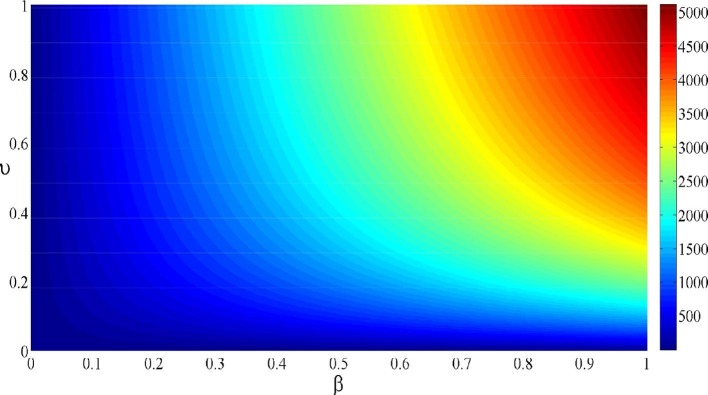
Fig. 2 illustrates the contour plot of $R_0$, we observe that for $\beta =1$ and $\upsilon =0$ the value of $R_0$ reaches the maximum value $5.11\times {10}^3$. By decreasing $\beta$ and $\upsilon$ from 1 to 0, we remark that the value of $R_0$ decreases also and tends toward $8.75\times {10}^{-3}$ (corresponding to $\beta =0\text{;}\upsilon =0$). This result reflects the impact of these two key parameters in controlling the infection.

Fig. 2.

Contour plot of $R_0$ depending on $\beta$ and $\upsilon$.

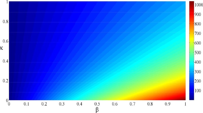
From the contour plot of $R_0$ given in Fig. 3 , we observe that for $\beta =1$ and $\kappa =0$ the value of $R_0$ reaches the maximum value $1.03\times {10}^3$. When the parameter $\kappa$ is increased from 0 to 1 and the parameter $\beta$ is decreased also from 1 to 0, we observe that f $R_0$ gradually decreases and tends to the limit value $1.93\times {10}^{-1}$ (corresponding to $\beta =0\text{;}\kappa =1$). Hence, the parameters x and y play an essential role in controlling the infection spread.

Fig. 3.

Contour plot of $R_0$ depending on $\beta$ and $\kappa$.

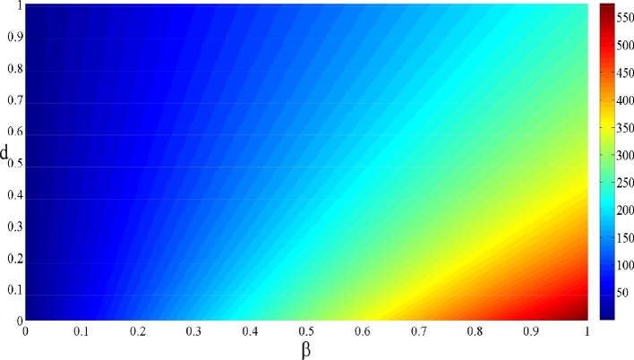
The last contour plot of $R_0$ in illustrated in Fig. 4 . We observe that when $\beta =1$ and $d=0$ the value of $R_0$ reaches its maximal value of $5.74\times {10}^2$. By decreasing $\beta$ from 1 to 0 and increasing d from 0 to 1, we observe that the value of $R_0$ gradually decreases and tends towards $1.57\times {10}^{-1}$ (corresponding to $\beta =0\text{;}d=1$). This confirm the impact of the $\beta$ and d in controlling the progression of the infection.

Fig. 4.

Contour plot of $R_0$ depending on $\beta$ and d.

Numerical simulations and discussion

This section will illustrate our mathematical results by different numerical simulations. To this end, we will apply the algorithm given in [42] to solve the system (2). The parameters of our model representing the infection and the recovery rates are estimated from COVID-19 Morocco case [43]. The different used values of our parameters in our numerical simulations are given in Table 1.

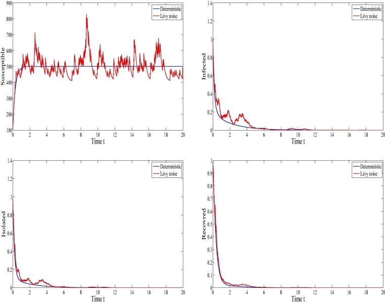
Figure 5 shows the dynamics of COVID-19 infection during the period of observation for the case of the disease extinction. From this figure, we clearly observe that the curves representing to the deterministic model converge towards the endemic-free equilibrium $E_f=\left(5.1\times {10}^2,0,0,0\right)$. The curves that represent the stochastic model fluctuate around the curves representing the deterministic ones. Moreover, it will be worthy to notice that in this case, the susceptible increase to reach their maximum and the other SIQR components that are the infected, the quarantined (the isolated) and the recovered vanish which means that the disease dies out. Within the used parameters in this figure (see Table 1), we have $R_0=0.95<1$ which indicates the die out of the infection. This is consistent with our theoretical findings concerning the extinction of SIQR infection.

Fig. 5.

The evolution of the infection when $R_0=0.95$.

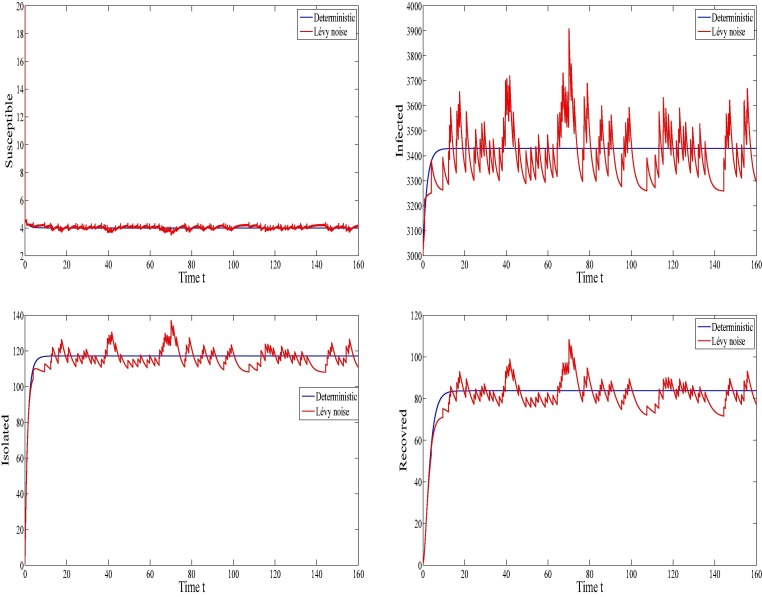
The evolution of the infection for both the deterministic model and the stochastic with Lévy jumps model is illustrated in Fig. 6 in the case of the disease persistence. Regarding the depicts of this figure, we can see that the plots corresponding to the deterministic model converge towards the endemic equilibrium $E^{\ast }=\left(4,3.42\times {10}^3,117.17,83.69\right)$. The fluctuation around the endemic equilibrium $E^{\ast }$ is clearly remarked for the stochastic numerical results. We note that in this epidemic situation, all the four SIQR compartments, i.e. the susceptible, the infected, the quarantined (the isolated) and the recovered remain at constant level which means that the disease persists. Within the used parameters in this figure (see Table 1), we have $R_0=31.12>1$ which indicates the persistence of the infection. This is consistent with our theoretical findings concerning the infection persistence.

Fig. 6.

The evolution of the infection when $R_0=31.12$.

Conclusion

In this present work, a stochastic coronavirus model with Lévy noise is presented and analyzed. We have given a four compartments SIQR model representing the interaction between the susceptible, the infected, the quarantined (the isolated) and the recovered. A white noise as well as a Lévy jump perturbations are incorporated in all model compartments. We have proved the existence and the uniqueness of the global positive solution for the stochastic COVID-19 epidemic model which ensures the well-posedness of our mathematical model. By using some appropriate functionals, we have shown that the solution fluctuates around the steady states under sufficient conditions. Different numerical results support our theoretical findings. Indeed, the extinction of the disease is observed for the basic reproduction number less than unity. However, the persistence of the disease is observed for the basic reproduction number greater than one. Moreover, the fluctuation of the stochastic solution around the disease-free equilibrium is observed for the extinction case and the fluctuation of the stochastic solution around the endemic equilibrium is observed for the persistence case.

Funding

None.

CRediT authorship contribution statement

Jaouad Danane: Conceptualization, Writing - original draft, Software. Karam Allali: Conceptualization, Writing - original draft, Software. Zakia Hammouch: Writing - original draft, Software, Formal analysis, Visualization, Methodology. Kottakkaran Sooppy Nisar: Writing - original draft, Formal analysis, Software, Writing - review & editing.

Declaration of Competing Interest

The authors declare that they have no known competing financial interests or personal relationships that could have appeared to influence the work reported in this paper.

References

- 1.Wang Y., Jiang D., Alsaedi A., Hayat A. Modelling a stochastic HIV model with logistic target cell growth and nonlinear immune response function. Physica A. 2018;501:276–292. [Google Scholar]
- 2.Sun Q., Min L., Kuang Y. Global stability of infection-free state and endemic infection state of a modified human immunodeficiency virus infection model. IET Syst Biol. 2015;9(3):95–103. doi: 10.1049/iet-syb.2014.0046. [DOI] [PMC free article] [PubMed] [Google Scholar]
- 3.Allali K., Danane J., Kuang Y. Global Analysis for an HIV Infection Model with CTL Immune Response and Infected Cells in Eclipse Phase. Appl Sci. 2017;7:861. [Google Scholar]
- 4.Danane J., Allali K. Optimal control of an HIV model with CTL cells and latently infected cells. Numerical Algebra Control Optim. 2020;10(2):207. [Google Scholar]
- 5.Wang K., Wang W., Liu X. Global stability in a viral infection model with lytic and nonlytic immune responses. Comput Math Appl. 2006;51(9–10):1593–1610. [Google Scholar]
- 6.Li M., Zu J. The review of differential equation models of HBV infection dynamics. J Virol Methods. 2019 doi: 10.1016/j.jviromet.2019.01.014. [DOI] [PubMed] [Google Scholar]
- 7.Rajaji R., Pitchaimani M. Analysis of stochastic viral infection model with immune impairment. Int J Appl Comput Math. 2017;3(4):3561–3574. [Google Scholar]
- 8.Kermack W.O., McKendrick A.G. A contribution to the mathematical theory of epidemics. Proc R Soc London A. 1927;115(772):700–721. [Google Scholar]
- 9.Yosyingyong P., Viriyapong R.J. Global stability and optimal control for a hepatitis B virus infection model with immune response and drug therapy. Appl Math Comput. 2018 doi: 10.1007/s12190-018-01226-x. [DOI] [PubMed] [Google Scholar]
- 10.Danane J., Allali K. Mathematical Analysis and Treatment for a Delayed Hepatitis B Viral Infection Model with the Adaptive Immune Response and DNA-Containing Capsids. High-Throughput. 2018;7(4):35. doi: 10.3390/ht7040035. [DOI] [PMC free article] [PubMed] [Google Scholar]
- 11.Zheng Y., Min L., Ji Y., Su Y., Kuang Y. Global stability of endemic equilibrium point of basic virus infection model with application to HBV infection. J Syst Sci Complex. 2010;23:1221–1230. [Google Scholar]
- 12.Danane J., Allali K., Hammouch Z. Mathematical analysis of a fractional differential model of HBV infection with antibody immune response. Chaos Solitons Fractals. 2020;136 [Google Scholar]
- 13.Gonzalez R.E.R., Coutinho S., Zorzenon dos Santos R.M., de Figueiredo P.H. Dynamics of the HIV infection under antiretroviral therapy: a cellular automata approach. Physica A. 2013;392(19):4701–4716. [Google Scholar]
- 14.Wang Y., Jiang D., Hayat T., Ahmad B. A stochastic HIV infection model with T-cell proliferation and CTL immune response. Appl Math Comput. 2017;315:477–493. [Google Scholar]
- 15.Liang Y., Greenhalgh D., Mao X. A stochastic differential equation model for the spread of HIV amongst people who inject drugs. Comput Math Methods Med. 2016;:14. doi: 10.1155/2016/6757928. Article ID 6757928. [DOI] [PMC free article] [PubMed] [Google Scholar]
- 16.Meskaf A., Tabit Y., Allali K. Global analysis of a HCV model with CTL, antibody responses and therapy. Appl Math Sci. 2015;9:3997–4008. [Google Scholar]
- 17.Yousfi N., Hattaf K., Rachik M. Analysis of a HCV model with CTL and antibody responses. Appl Math Sci. 2009;3(57):2835–2845. [Google Scholar]
- 18.Dahari H., Lo A., Ribeiro R.M., Perelso A.S. Modeling hepattis C virus dynamics: Liver regeneration and critical drug efficacy. J Theor Biol. 2007;247:371–381. doi: 10.1016/j.jtbi.2007.03.006. [DOI] [PMC free article] [PubMed] [Google Scholar]
- 19.Reluga T.C., Dahari H., Perelson A.S. Analysis of hepatitis c virus infection models with hepatocyte homeostasis. SIAM J Appl Math. 2009;69(4):999–1023. doi: 10.1137/080714579. [DOI] [PMC free article] [PubMed] [Google Scholar]
- 20.Bai Y, Yao L, Wei T, et al. Presumed asymptomatic carrier transmission of COVID-19. JAMA. Published online February 21, 2020.https://doi.org/10.1001/jama.2020.2565. [DOI] [PMC free article] [PubMed]
- 21.Heymann D.L., Shindo N. COVID-19: what is next for public health? Lancet. 2020;395(10224):542–545. doi: 10.1016/S0140-6736(20)30374-3. [DOI] [PMC free article] [PubMed] [Google Scholar]
- 22.Di Giamberardino P., Iacoviello D. Evaluation of the effect of different policies in the containment of epidemic spreads for the COVID-19 case. Biomed Signal Process Control. 2020;65 doi: 10.1016/j.bspc.2020.102325. [DOI] [PMC free article] [PubMed] [Google Scholar]
- 23.Atangana E., Atangana A. Facemasks simple but powerful weapons to protect against COVID-19 spread: can they have sides effects? Results Phys. 2020 doi: 10.1016/j.rinp.2020.103425. [DOI] [PMC free article] [PubMed] [Google Scholar]
- 24.Chan J.F., Yuan S., Kok K.H., To K.K., Chu H., Yang J., et al. A familial cluster of pneumonia associated with the 2019 novel coronavirus indicating person-to-person transmission: a study of a family cluster. Lancet. 2020;395(10223):514–523. doi: 10.1016/S0140-6736(20)30154-9. [DOI] [PMC free article] [PubMed] [Google Scholar]
- 25.Wan H, Cui JA, Yang GJ. Risk estimation and prediction by modeling the transmission of the novel coronavirus (COVID-19) in mainland China excluding Hubei province (2020).https://doi.org/10.1101/2020.03.01.20029629. medRxiv. [DOI] [PMC free article] [PubMed]
- 26.Goufo E.F.D., Khan Y., Chaudhry Q.A. HIV and shifting epicenters for COVID-19, an alert for some countries. Chaos Solitons Fractals. 2020;139 doi: 10.1016/j.chaos.2020.110030. [DOI] [PMC free article] [PubMed] [Google Scholar]
- 27.Atangana A., Araz S.İ. Mathematical model of COVID-19 spread in Turkey and South Africa: theory, methods, and applications. Adv Difference Equations. 2020;2020(1):1–89. doi: 10.1186/s13662-020-03095-w. [DOI] [PMC free article] [PubMed] [Google Scholar]
- 28.Faraz N, Khan Y, Goufo ED, Anjum A. Dynamic analysis of the mathematical model of COVID-19 with demographic effects. Zeitschrift für Naturforschung C, 1(ahead-of-print); 2020. [DOI] [PubMed]
- 29.Jia J, Ding J, Liu S, Liao G, Li J, Duan B, Zhang. Modeling the Control of COVID-19: impact of policy interventions and meteorological factors. Electron J Differ Equations 23;2020:1–24.
- 30.Borah M.J., Hazarika B., Panda S.K., Nieto J.J. Examining the correlation between the weather conditions and COVID-19 pandemic in India: a mathematical evidence. Results Phys. 2020;19 doi: 10.1016/j.rinp.2020.103587. [DOI] [PMC free article] [PubMed] [Google Scholar]
- 31.Volpert V., Banerjee M., Petrovskii S. On a quarantine model of coronavirus infection and data analysis. Math Model Natural Phenomena. 2020;15(24):1–6. [Google Scholar]
- 32.Wu L.I., Feng Z. Homoclinic bifurcation in an SIQR model for childhood diseases. J Differ Eqs. 2000;168(1):150–167. [Google Scholar]
- 33.Pitchaimani M., Brasanna D.M. Effects of randomness on viral infection model with application. IFAC J Syst Control. 2018;6:53–69. [Google Scholar]
- 34.Mahrouf M., El Mehdi L., Mehdi M., Hattaf K., Yousfi N. A stochastic viral infection model with general functional response. Nonlinear Anal Differ Eqs. 2016;4(9):435–445. [Google Scholar]
- 35.Zhang Q, Zhou K. Stationary distribution and extinction of a stochastic SIQR model with saturated incidence rate. Math Problems Eng 2019;2019, Article ID 3575410, 12 pages.
- 36.Liu Q., Jiang D., Shi N. Threshold behavior in a stochastic SIQR epidemic model with standard incidence and regime switching. Appl Math Comput. 2018;316:310–325. [Google Scholar]
- 37.Zhang X., Wang K. Stochastic model for spread of AIDS driven by Lévy noise. J Dyn Differ Eqs. 2015;27:215–236. [Google Scholar]
- 38.Zhang X., Jiang D., Hayat T., Ahmad B. Dynamics of a stochastic SIS model with double epidemic diseases driven by Lévy jumps. Physica A. 2017;471:767–777. [Google Scholar]
- 39.Singh A., Razooky B., Cox C.D., et al. Transcriptional bursting from the HIV-1 pro- moter is a significant source of stochastic noise in HIV-1 gene expression. Bio- phys J. 2010;98(8):L32–L34. doi: 10.1016/j.bpj.2010.03.001. [DOI] [PMC free article] [PubMed] [Google Scholar]
- 40.Berrhazi B.E., El Fatini M., Laarib A., Pettersson R., Taki R. A stochastic SIRS epidemic model incorporating media coverage and driven by Lévy noise. Chaos Solitons Fractals. 2017;105:60–68. [Google Scholar]
- 41.Feng Z., Thieme H.R. Recurrent outbreaks of childhood diseases revisited: the impact of isolation. Math Biosci. 1995;128(1–2):93–130. doi: 10.1016/0025-5564(94)00069-c. [DOI] [PubMed] [Google Scholar]
- 42.Zou X., Wang K. Numerical simulations and modeling for stochastic biological systems with jumps. Commun Nonlinear Sci Numer Simul. 2014;19:1557–1568. [Google Scholar]
- 43.Statistics of health ministry of Morocco:www.sante.gov.ma,www.covidmaroc.ma.