

SUMMARY
Learning valence-based responses to favorable and unfavorable options requires judgments of the relative value of the options, a process necessary for species survival. We have found, using engineered mice, that circuit connectivity and function of the striosome compartment of the striatum are critical for this type of learning. Calcium imaging during valence-based learning exhibited a selective correlation between learning and striosomal, but not matrix, signals. This striosomal activity encoded discrimination learning and was correlated with task engagement, which could, in turn, be regulated by chemogenetic excitation and inhibition. Striosomal function during discrimination learning was disturbed with aging, and severely so in a mouse model of Huntington’s disease. Anatomical and functional connectivity of parvalbumin-positive, putative fast-spiking interneurons (FSIs) to striatal projection neurons was enhanced in striosomes compared to matrix in mice that learned. Computational modeling of these findings suggests that FSIs can modulate striosomal signal-to-noise ratio, crucial for discrimination and learning.
Keywords: Corticostriatal, approach-avoidance, cost-benefit, decision-making, utility, subjective value, motivation, parvalbumin interneurons, VGluT1, excitation-inhibition balance
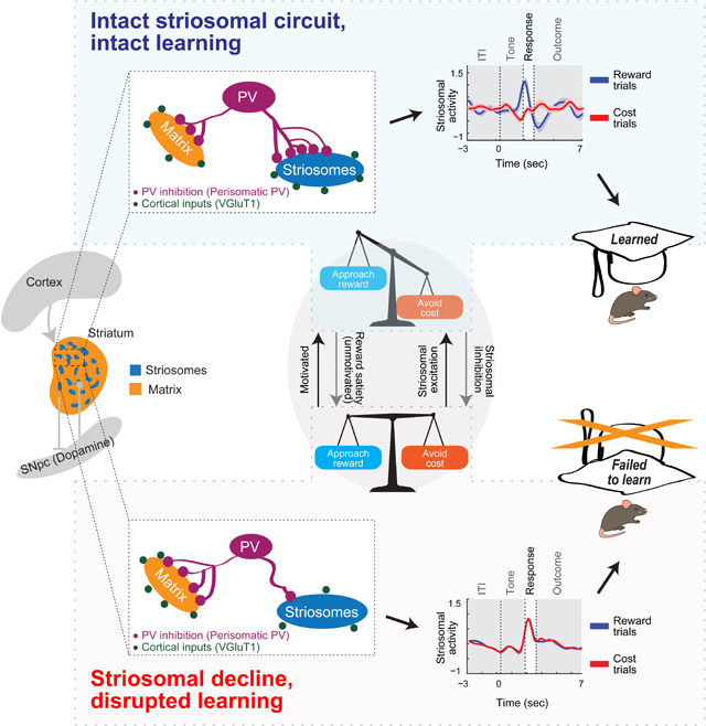
Graphical Abstract
eTOC blurb
Friedman and Hueske et al. find that specialized regions of the striatum, a key part of the brain’s movement and motivation control system, are essential for learning about the values of good and bad outcomes of decisions. The learning signals in these striosomes, unlike in the surrounding matrix, scale according to subjective value and are vulnerable to decline with aging and neurodegenerative disorders. Striosomal signal-to-noise ratio improves with learning, and local inhibition, via parvalbumin-positive interneurons.
INTRODUCTION
The striatum is a key input-output structure of the basal ganglia and is the origin of movement- and motivation-modulating output circuits affected in disorders including Parkinson’s disease, Huntington’s disease (HD) and a remarkable range of other disorders affecting motoric, affective, and cognitive functions (Alexander and Crutcher, 1990; Bates et al., 2015; Gittis and Kreitzer, 2012; Gleichgerrcht et al., 2010; Nelson and Kreitzer, 2014). Striatal neurons have multiple phenotypes including principal projection neurons (SPNs), subdivided into dopamine D1 receptor-expressing (direct pathway) and dopamine D2 receptor-expressing (indirect pathway) neurons, and multiple interneuronal subtypes (Kreitzer and Berke, 2011; Miyamoto et al., 2018; Surmeier et al., 2007; Tepper and Bolam, 2004). A prominent second dimension of striatal organization is represented by its neurochemically distinct compartments, distinguished by a labyrinthine striosome compartment embedded in a larger surrounding matrix compartment (Brimblecombe and Cragg, 2017; Cox and Witten, 2019; Crittenden and Graybiel, 2011; Graybiel and Ragsdale, 1978). These compartments, the main focus of our study, are the least well understood of these striatal subdivisions, with only emerging studies of their functions (Bloem et al., 2017; Friedman et al., 2017; Friedman et al., 2015a; McGregor et al., 2019; Xiao et al., 2020; Yoshizawa et al., 2018). It is known, however, that striosomes and matrix each have distinct patterns of development (Graybiel and Hickey, 1982; Kelly et al., 2018; Lanca et al., 1986; Matsushima and Graybiel, 2020), neurotransmitter expression (Graybiel, 1995), input-output connections, and single-nucleus mRNA signatures identified by snRNA-seq (Gokce et al., 2016; Märtin et al., 2019; Saunders et al., 2018).
Critical evidence suggests that striosomal SPNs (sSPNs) project directly to dopamine-containing neurons of substantia nigra pars compacta (SNpc) (Crittenden et al., 2016; Evans et al., 2020; Fujiyama et al., 2011; Watabe-Uchida et al., 2012) and also to lateral habenula (Hong et al., 2019; Rajakumar et al., 1993; Stephenson-Jones et al., 2013), both implicated in reinforcement signaling, reward-based learning, and behavioral choice (e.g., Hikosaka, 2010; Schultz, 2016), as well as the impetus to move (e.g., da Silva et al., 2018; Howe and Dombeck, 2016). Moreover, striosomes receive inputs from cortical and subcortical regions related to the limbic system (Crittenden and Graybiel, 2011; Eblen and Graybiel, 1995). These remarkable circuit connections of striosomes make them well-placed to influence value-related learning and decision-making modulated by motivation. Available evidence suggests that striosomes and striosome-based circuits are differentially implicated in reinforcement-related updating paradigms (Bloem et al., 2017; Yoshizawa et al., 2018), and that they influence cost-benefit conflict decision-making in both non-human primates (Amemori and Graybiel, 2012; Amemori et al., 2018; Amemori et al., 2020) and rodents (Friedman et al., 2017; Friedman et al., 2015a).
These studies were performed in well-trained subjects, leaving it unclear what functions striosomes might perform during the process of learning how to decide in the face of potential rewarding and costly outcomes, a central focus here. Such functions are susceptible to decline with aging and in age-related neurodegenerative disorders, but again, little is known about the relative contributions of striosomes and matrix to these impairments. Evidence from studies of postmortem brains of HD patients with early onset and with histories of mood abnormalities (Hedreen and Folstein, 1995; Tippett et al., 2007) has implicated differential striosomal vulnerability. In addition, the ability to develop effective decision-making strategies based on expected value not only declines with age (Tymula et al., 2013), but also in the wake of neurodegenerative disorders, including in HD (Gleichgerrcht et al., 2010; Perry and Kramer, 2015; Walker, 2007).
Here, we investigated the neurobiology of decision-making during valence-discriminaton learning across healthy aging and in a mouse model of HD relying on mouse engineering and a combination of functional, behavioral and anatomical methods. We further tracked the activity of striatal microcircuits interconnecting striosomes including striatal parvalbumin (PV) interneurons (Friedman et al., 2017; Friedman et al., 2015a; Gittis and Kreitzer, 2012) known to be affected in HD and HD models (Cepeda et al., 2013; Holley et al., 2019; Indersmitten et al., 2015; Lallani et al., 2019; Reiner et al., 2013). Our findings demonstrate that striosomal circuits, modulated by putative PV interneurons, underpin the capacity for reinforcement-driven valence discriminaton learning and engagement under normal conditions and that these circuits are differentially vulnerable through the course of aging and in an HD context.
RESULTS
Striosomal Activity, but Not Matrix Activity, Is Shaped by Discrimination Learning
In the behavioral task (Figure 1A), each mouse was presented with one of two tones (4 or 8 kHz for 2 s), indicating either reward delivery (tone 1; 4, 12 or 24 μl of 10% sucrose) or cost delivery (tone 2; 4, 40 or 400 lux of light from an LED panel facing the mouse), followed by a 1-s response period. Depending on the auditory cue, mice could maximize reward delivery by licking more during the response period to tone 1, and could minimize aversive light exposure by licking less during the response period to tone 2 during each trial of the 150-trial sessions. As daily training proceeded, we estimated their response-period (RP) licking patterns, that is, the time between tone off and reinforcement. We required that the difference developed by individual mice in RP lick rate distributions between reward and cost trials meet significance (p < 0.05, Kolmogorov-Smirnov [K-S] test; Figures 1B, 1C, and S1A–S1C) to qualify as having met learning criterion. We measured these both across training and during reversal learning of cue-outcome contingencies (Figure S1D).
Figure 1. Striosomal Transients Are Selectively Modified by Learning.
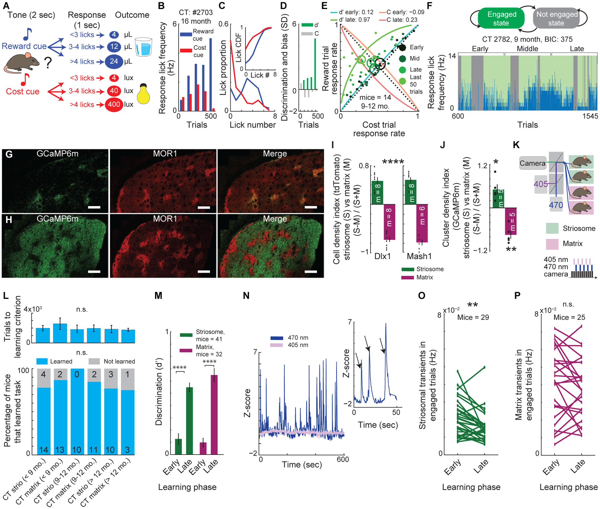
(A) Discrimination task.
(B-D) Licking response across learning (B), learning criterion defined by K-S test of cost and reward lick distributions (C), and discrimination index (d’) and response bias (“C”) in a typical mouse (D).
(E) During learning, d’ increases as reward response rate increases and cost response rate decreases (blue to green arc concavity), separable from changes in response bias, “C”, (orange to red arc concavity). We split learning into three phases and calculated the mean (ellipse center) and SEM (ellipse size) of d’ for each phase. Dots: performance of individual mice during given phase.
(F) HMM model assigns trials as engaged or not engaged state (top). Progression of a mouse from naïve to learning criterion and state assignments of trials (bottom).
(G and H) Striosomal (G) and matrix (H) Flp-expressing mice injected with Flp-dependent GCaMP6m virus. Scale bar, 200 μm.
(I) Ratio of tdTomato+ cell density in striosomes (S) and matrix (M) calculated for Dlx1-CreER;Ai14 and Mash1-CreER;Ai14 mice with tamoxifen induction at E11 or E15 (mean ± SEM, one-way ANOVA, striosomes vs. matrix ****p < 0.0001). Dots: individual mice (m).
(J) Specificity of GCaMP6m expression with tamoxifen induction on E11 and E15 (one-sample t-test compared to zero, *p = 0.0198, **p = 0.0022). See ‘Quantifying Density of GCaMP6m+ Cells in Striosome and Matrix Compartments in E11/E15 Model Mice’ in STAR Methods.
(K) Fiber photometry setup.
(L) Percentage of mice that learned the task (bottom; chi-square test) and number of sessions to learn (top; 2-way ANOVA) were not different across age and compartment in CT mice.
(M) d’ in the first (early) and last (late) 200 trials of learning in CT mice (2-way ANOVA, ****p < 0.0001).
(N) Example of 470 nm GCaMP6m Ca++ transients and control 405 nm signal. Insert magnifies 470 nm signal. Arrows: Ca++ transients.
(O and P) Striosomal (O; paired t-test, **p = 0.0025), but not matrix (P; p = 0.18), transient frequency during engaged trials decreased across learning. Lines: individual mice.
We used a standard signal detection theoretic (SDT) approach to evaluate discrimination as a measure of learning (d’), and response bias as a measure of task-engagement (C) (Figures 1D and 1E) (e.g., Berditchevskaia et al., 2016b). We applied a hidden Markov model (HMM)-based approach, modified to accommodate the dynamic process of learning (e.g., Friedman et al., 2016) in order to assign, trial-by-trial, the behavior of mice as being in an engaged state or not in an engaged state (Figures 1F and S1E–S1H; see STAR Methods).
To tag and characterize striatal compartments (Figures S1I–S1T), we crossed inducible Mash1(Asc1)-CreER (Kim et al., 2011) or Dlx1-CreER (Taniguchi et al., 2011) mice with mice from a line encoding a Cre-dependent Flp recombinase (LSL-Flpo), and then we administered to the pregnant dams tamoxifen to induce Cre recombinase activity at embryonic timepoints targeting the birthdates of striosomal (~E11) or matrix (~E15) populations (Bloem et al., 2017; Kelly et al., 2018; Matsushima and Graybiel, 2020). We called these lines ‘striosome’ and ‘matrix’ lines, with the understanding that full selectivity cannot be achieved by these methods (STAR Methods). To perform photometric recordings of striosomal and matrix calcium transients, we injected the anterior dorsomedial striatum (DMS) of these striosomal or matrix birthdate-labeled mice with AAV8-EF1a-fDIO-GCaMP6m (AAV8 viral vector encoding a Flp-dependent construct of genetically encoded calcium indicator, GCaMP6m; Figures 1G–J and S1U–S1AF). We found that compartmental selectivity corresponded to ~75% of labeled cells or GCaMP6m-positive (+) cells residing in striosomes in striosome-labeled mice and ~85% residing in matrix in matrix-labeled mice (Figures 1I–J and S1S–S1W) indicating high compartmental selectivity for both mouse lines.
We simultaneously recorded neural activity and behavioral performance as mice acquired valence-based associations (Figures 1K–1P and S2A–S2L). We found no behavioral differences between striosomal and matrix mice in the acquisition of valence-based discrimination, task engagement, licking rates, or learning rates (Figures 1L, 1M and S2A–S2C). Strikingly, however, in photometric recordings of striatal compartments across learning, in the majority of striosome mice, the frequency of striosomal Ca++ transients declined (27% decrease on average, p = 0.0024), but no such changes were detected in matrix mice (Figures 1O and 1P). By contrast, amplitudes of transients in striosomes were significantly higher than those in matrix (p < 0.0001; Figure S2M), and these amplitudes trended higher across learning (p = 0.09), unlike those in matrix (p = 0.25; Figures S2N and S2O). In striosome mice, but not in matrix mice, signal-to-noise ratio (SNR) of transients also increased with learning (p = 0.017; Figure S2P). These results demonstrated that striosomal signals were selectively modified during discrimination learning, with their numbers declining but their amplitudes increasing.
Striosomes, but Largely Not Matrix, Encode Discrimination Levels during Learning
We next asked, again with targeting of anterior DMS, whether striosomal activity were related to the degree of discrimination learning attained. In individual striosome mice, the difference in RP activity between reward and cost trials (R−CRP), measured as the average integrated activity in reward-trial RP minus that in cost-trial RP, was larger when d’ was high than when d’ was low, regardless of high or low numbers of response licks. Further, striosomal, but not matrix, R−CRP values were larger toward the end of learning (Figures 2A, 2B, S2Q, and S2R). Lick rates were negatively correlated with activity in striosome mice during the RP in cost trials (CRP) and correlated positively during the RP in reward trials (RRP). These results indicate that licking frequencies cannot explain striosomal activity. By contrast, a positive correlation between lick rates and matrix neural activity occurred only in reward trials (Figure S2S).
Figure 2. Striosomes, but not Matrix, Encode Discrimination Learning.
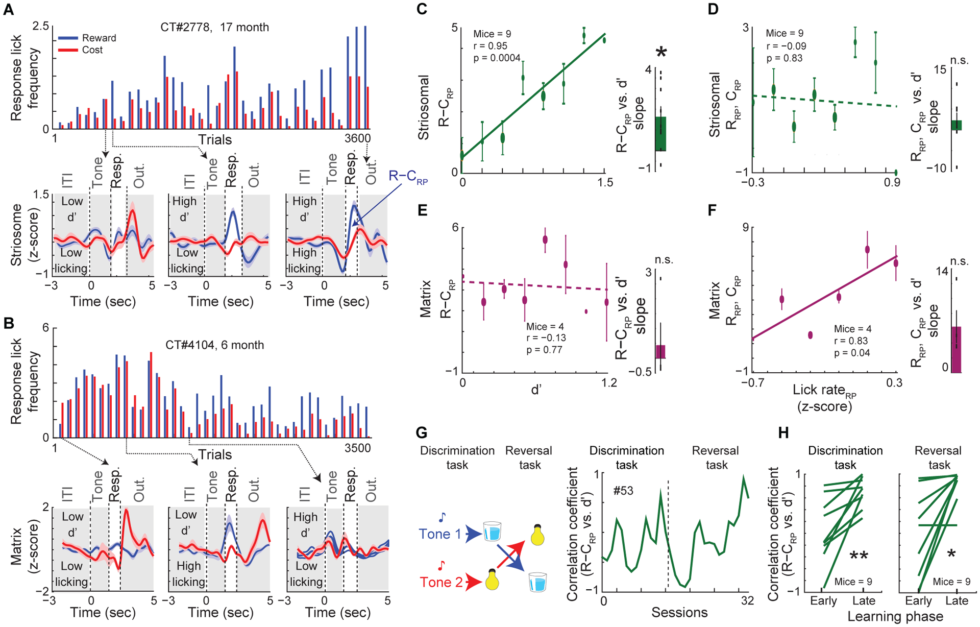
(A and B) Striosome (A) and matrix (B) mouse RP lick frequency (top) and photometric recordings for selected bins (bottom). Response period (white); other periods (gray).
(C) Correlation between striosomal R−CRP and d’ across trials (left, mean ± SEM, Pearson correlation) and average correlation slopes across mice (right, Wilcoxon signed-rank test, *p = 0.01).
(D) Correlation of striosomal RP activity (RRP, CRP) with RP lick rates across trials (left) and average correlation slopes across mice (right). The correlations of photometric signals with lick rates were restricted to the first quarter of trials to reach learning criterion, presumably before d’ and lick rates also begin to correlate.
(E and F) Same as C and D but for matrix transients.
(G) After training to learning criterion, cue-outcome contingencies were reversed (left). Correlation coefficient between R−CRP and d’ in a striosome mouse (right; dashed line indicates task switch).
(H) Maximum correlation coefficient between R−CRP and d’ in the first and last 25% of trials of discrimination learning (left; paired t-text, **p = 0.006) and reversal learning (right, *p = 0.01).
There was a remarkable contrast between the respective levels of correlation between d’ and striosomal or matrix R−CRP activity. In striosome mice, R−CRP signals were correlated with d’ (Pearson correlation, r = 0.95, p = 0.0004), but not with lick frequency (r = −0.09, p = 0.83; Figures 2C, 2D, and S2T). In matrix mice, R−CRP signals were not correlated with d’ but were positively correlated with RP lick rates (Figures 2E, 2F, and S2U). We performed conditional analyses to delineate more thoroughly correlations of striatal compartmental activity with licking behavior versus discrimination and confirmed that striosomal activity scaled with d’, but not with licking rates (Figure S2V–S2Y). As a control for the specificity of these effects to RP, we looked for, but failed to detect, such correlations in signals recorded during tone periods, outcome periods, or inter-trial intervals (ITI) of the task (Figures S2Z and S2AA), highlighting the importance and selectivity of striosomal function during RP related to learning of this task. The emergence of correlations across learning between d’ and striosomal R−CRP grew in almost all of striosome birthdate-labeled mice: striosomal signals tracked initial discrimination (n = 9/9), and re-emerged during reversal (n = 8/9) learning (Figures 2G, 2H, and S3A–S3D).
This striosome-specific correlation between R−CRP and d’ was equally strong in two independent CreER birthdate-labeled lines, Dlx1-CreER and Mash1-CreER lines (Bloem et al., 2017; Kelly et al., 2018) used to label striosomes. These lines had differing proportions of cells expressing D1 and D2 receptors in striosomes (E11-tagged Dlx1 D1 proportion: min-to-max = 0.37–0.62, mean ± SEM = 0.51 ± 0.09; E11-tagged Mash1 D1 proportion: min-to-max = 0.50–0.93, mean ± SEM = 0.66 ± 0.16; Figures S3E, S1M, and S1O). Thus, there was not a clear and close correlation between the similar striosomal encoding of learning in the two lines and the proportion of cells expressing D1 and D2 receptors (Figures 1L, 1M, S2A–S2C, and S1M–S1T). These findings suggest that striosomal activity, as measured in the birthdate-labeled striosome mice, but not matrix activity, as measured in the birthdated-labeled matrix mice, is correlated with d’ during acquisition of the valence discrimination task.
Striosomal Activity Reflects Task Engagement and Expected Outcome Valence and Value
To be successful in the task, both engagement in the task and assessment of the outcome value associated with each cue were necessary. The positive striosomal R−CRP correlation with d’ was significantly stronger when photometric signals were filtered for HMM-assigned engaged state (~3x stronger, p = 0.11 for not engaged, 0.01 for engaged), suggesting that engagement and task learning were aligned (Figures S3F–S3H).
We examined striosomal activity across binned levels of licking responses to cost and reward cues (Figure 3A). Striosomal RRP activity became increasingly positive as mice licked more to receive greater positive outcomes, but striosomal CRP activity became increasingly negative in cases in which mice licked more in advance of greater aversive outcomes. The opposite modulation of striosomal signals in reward and cost trials, a modulation not seen in matrix (Figure 3A), reinforces the view that striosomal signals do not reflect motor lick behavior to a degree detectable by our methods. Moreover, task engagement cannot be the sole driver of this modulation, given the more negative CRP signals with greater lick activity on cost trials. Instead, our fiindings suggest that striosomal signals reflect expected outcome valence (positive in advance of reward, negative in advance of cost) as well as value (signals are more strongly positive or negative with greater expected reward or greater expected cost). The matrix compartment appeared sensitive only to expected positive outcome.
Figure 3. Striosomal Activity Reflects Subjective Value and Causally Modulates Engagement.

(A) Striosomal and matrix RRP increased with increasing reward level (one-way ANOVA, p < 0.001), but only striosomal CRP decreased with increasing cost level (striosomes: p = 0.0075; matrix: p = 0.29).
(B and C) Reward devaluation by giving free access to sucrose (B) or water (C) before test sessions after criterion decreased task engagement (gray ramp) and striosomal RRP (Pearson correlation), relative to sessions in which learning criterion was reached. ↑E: more engagement; ↓E: less engagement. Dots: individual mice.
(D) Diazepam (0.5 mg/kg, 10 min pre-session) increased task engagement (gray ramp) and striosomal RRP (Pearson correlation).
(E) Striosomal (left), but not matrix (right), RRP increased with task engagement in CT mice. E: engaged; NE: not engaged.
(F-H) Flp-dependent GCaMP6m and DREADD-mCherry constructs co-expressed in striosome (G) and matrix (H) mice allowed compartment-specific manipulation and photometry recording (F). Selectivity was examined with MOR1 striosomal marker. Scale bar, 200 μm.
(I) Ca++ transients in a striosome mouse expressing inhibitory DREADD after CNO (blue) or saline (green) injection.
(J) Transient rate decreased across mice after CNO injection (**p = 0.003, paired t-test). Each line shows a saline-CNO session pair.
(K and L) In striosome (K), but not matrix (L), mice expressing inhibitory DREADD, CNO injection decreased Ca++ transient rate and task engagement (higher C; Pearson correlation).
(M and N) Same as I and J, but in mice expressing excitatory DREADD. Transient rate increased after CNO (orange) compared to saline (green) injection (**p = 0.001).
(O and P) In striosome (O), but not matrix (P), mice expressing excitatory DREADD, CNO increased Ca++ transient rate and task engagement (lower C; Pearson correlation).
To test how manipulating outcome value would affect striosomal signals, we implemented a reward devaluation protocol. Prior to discrimination task sessions, we satiated mice with either sucrose or water in their home cage (STAR Methods). We found a selective decrease in striosomal activity in RRP, but not CRP, signals, accompanied by a reduction in task engagement. No such modulation was detectable in matrix activity in devaluation protocols (Figures 3B, 3C, and S3I–S3K). Again recording in anterior DMS, we examined the effects of treatment with the anxiolytic, diazepam. In striosomes, this treatment increased both RRP and CRP signal amplitudes in proportion to increased task engagement, but in matrix, signal amplitudes were not detectably influenced by diazepam (Figures 3D and S3L–S3N). Thus, as task engagement was driven down by reward devaluation and was driven up by anxiolytic treatment, striosomal signals changed in tight correlation, suggesting that signals in striosomes, unlike those in matrix, integrate or reflect subjective value.
Finally, we asked whether task engagement exhibited by individual mice correlated with their striosomal and matrix RP signals (n = 37 striosome and 32 matrix mice). For reward trials, we found that striosomal RRP signals correlated positively with task engagement, so that mice that were more task-engaged had larger striosomal RP signals. Remarkably, no such correlation was found for matrix signals in our striatal region of study (Figure 3E). Together with findings from devaluation experiments, these findings indicate that striosomal, but not appreciably matrix, signals are sensitive to task engagement and reflect subjective value.
Chemogenetic Manipulation of Striosomes, but Not of Matrix, Can Causally Decrease or Increase Task Engagement
This correlational work did not ensure causality. We therefore applied chemogenetic methods, expressing designer receptors exclusively activated by designer drugs (DREADDs) selectively in striosomal or matrix neurons, and then modulated their activity with the DREADD ligand clozapine-N-oxide (CNO) (Roth, 2016). We expressed Flp-dependent inhibitory DREADD constructs (AAV8-EF1a-fDIO-hM4Di-mCherry) in mice with Flp-expressing striosomal or matrix populations while recording photometrically from these compartments. We found ~80% colocalization between DREADD and GCaMP6m viruses (Figures 3F–3H and S3O–Q). In striosome mice expressing inhibitory DREADDs, Ca++ transients were reduced with CNO treatment relative to saline administration in the same mice (n = 8 mice, p = 0.002, Figures 3I and 3J). The more the numbers of Ca++ transients decreased in striosomes, the more task engagement decreased (Figure 3K). No such effect was detectable with the same inhibitory DREADD manipulation of matrix populations (n = 5 mice, p = 0.71, Figure 3L).
Conversely, the numbers of Ca++ transients increased following CNO administration in striosome mice expressing excitatory DREADD constructs (AAV8-EF1a-fDIO-hM3Dq-mCherry) relative to the transient numbers in sessions in the same mice with saline instead of CNO administration (n = 4 mice, p = 0.04, Figures 3M and 3N). The more Ca++ transients increased in striosomes, the more task engagement increased (Figure 3O). No such effect was seen with excitatory manipulation of matrix populations (n = 6 mice, p = 0.3; Figure 3P).
These findings constitute evidence that a modulation of striosomal circuits drives a corresponding change in task engagement, so that inhibiting striosomes decreases task engagement, whereas exciting striosomes increases task engagement, effects not achieved by comparable modulation of matrix populations. Despite the ability to decrease and increase engagement, we failed to improve d’ and learning, perhaps due to DREADD manipulation not modulating the specific patterns of activity of striosomal neurons, a possibility that could be addressed by future methods.
Striosomal Discriminative R−CRP Activity Fails to Develop in Mice That Do Not Learn and Is Altered in Aged Mice
We next asked whether photometric striosomal signals were impacted by age or learning status. In younger aged control mice (age 6–12 mo.) that learned the discrimination task (CT-LY), there was a larger separation between striosomal signals in reward and cost trials than there was in older (age 13–21 mo.) mice (p < 0.05; Figure 4A). This difference appeared to be attributable to a more negative cost-trial activity in CT-LY mice relative to the cost-related signals in older aged mice that learned (CT-LO) (Figure 4B). In control mice that did not learn (CT-NL), the difference in striosomal R−CRP activity was scarcely divergent (Figure 4C). Nor were differences in R−CRP activity detectable in matrix populations regardless of age or learning status (Figures 4D, 4E, and S4A–S4C).
Figure 4. Striosomal but Not Matrix Activity Is Reduced in Aged Mice and Mice That Failed to Learn.
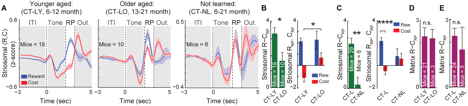
(A) In mice that learned the task, striosomal activity (mean ± SEM) during the cost-trial RP was suppressed more in younger (CT-LY) (left) than older (CT-LO) mice (middle). CT-NL mice (right) showed no difference between RRP and CRP.
(B) CT-LO (17.60 ± 0.56 months) mice showed reduced R−CRP signals (mean ± SEM) compared to CT-LY (7.42 ± 0.3 months) mice (left; *p = 0.024, Mann-Whitney test). In CT-LO mice, a lower suppression of CRP is responsible for the reduction in R−CRP area (right; *p < 0.05, 2-way ANOVA).
(C) Compared to CT-L mice (6–21 months), CT-NL mice (6–21 months) showed significantly lower R−CRP signals (left; **p < 0.01, Mann-Whitney test). CRP and RRP were significantly different in CT-L but not CT-NL mice (right; ****p < 0.0001, 2-way ANOVA).
(D and E) No difference in matrix R−CRP across age (D; p = 0.7421, Mann-Whitney test) or learning status (E; p = 0.5184).
We found a close correlation between striosomal R−CRP activity and engagement (C) in younger aged mice (CT-LY), but not in older aged mice (CT-LO mice) (Figures S4D–S4F). Only CT-LY mice showed modulation of d’ in relation to C (Figure S4G), consistent with the gating of learning by task engagement. Regardless of age, CT-L mice exhibited striosomal signals that correlated with d’, whereas CT-NL mice showed no such correlation (Figure S4H). These findings suggest that aging results in (1) less negative CRP striosomal activity, (2) reduced correlation between striosomal activity and task engagement, and (3) a lessened relationship between task engagement and learning.
Valence-Based Discrimination Correlates with Reward in Control Mice, but Correlates with Cost in HD Model Mice
We crossed the zQ175 knock-in HD model mouse line (Menalled et al., 2012) with our striosome and matrix lines to ask whether we could identify functional impairments at the level of compartmental deficits. A significantly lower proportion of the offspring of these crosses (here termed ‘HD mice’) achieved our learning criterion, including in reversal learning, compared to the proportion of CT mice that learned (Figures 5A, 5B, and S4I–S4K). These declines occurred despite the ability of HD mice to lick at normal rates during sucrose consumption, and despite their normal sensitivities to aversive and appetitive outcomes in the context of this task (Figures S4L–S4R).
Figure 5. Learning Correlates with Striosomal Reward-Trial Activity in CT Mice and with Cost-Trial Activity in HD Mice.
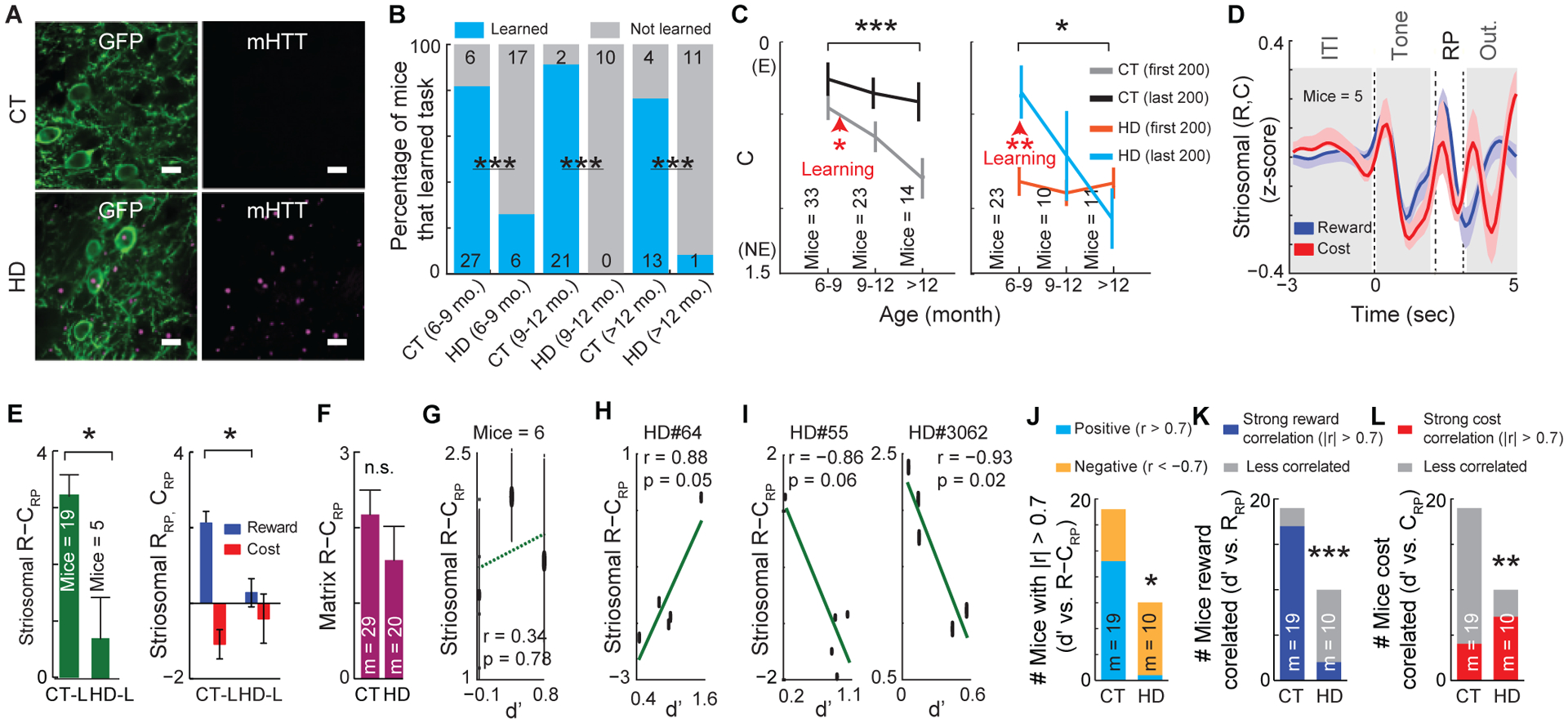
(A) Aggregates of mutant huntingtin (mHTT) protein (pink) present in GCaMP6m-expressing striosomal neurons (green) in HD but not in CT mice. Scale bar, 10 μm.
(B) Fewer HD mice met the discrimination learning criterion than CT mice (***p < 0.001, chi-square test).
(C) “C” (mean ± SEM) decreased with age in CT mice in early training but was restored with learning (left: ***p = 0.0009 for age, *p = 0.028 for learning, 2-way ANOVA). Only young HD mice restored initially low task engagement across learning (right: *p = 0.035 for age, **p = 0.0041 for young HD group, 2-way ANOVA and Bonferroni multiple comparisons test). Arrowheads: increased task engagement.
(D) Striosomal activity (mean ± SEM) of HD-L mice (6–12 months).
(E) HD mice, even those that learned, showed lower R−CRP (left: 6–12 months, *p = 0.012, Mann-Whitney test), largely due to reduced RRP (right: *p = 0.034, 2-way ANOVA and Bonferroni multiple comparisons test).
(F) No difference in matrix R−CRP between CT and HD mice (p = 0.1155, Mann-Whitney test, 6–21 months).
(G-I) Striosomal R−CRP and d’ were not correlated in HD-L mice as a group (G; Pearson correlation), but were correlated in individual mice. Examples of positive (H) and negative (I) correlations are shown.
(J) Among mice with strong correlations between striosomal R−CRP and d’ (Pearson correlation, |r| > 0.7), HD mice (10.1 ± 1.6 months) showed more negative correlations, whereas CT mice (11.9 ± 1.2 months) showed more positive correlations (*p = 0.023, chi-square test).
(K) Of mice shown in J, CT mice (11.9 ± 1.2 months) were more likely than HD mice (10.1 ± 1.6 months) to show strong (|r| > 0.7) RRP correlations with d’ (***p = 0.0002).
(L) HD mice were more likely than CT mice to show strong (|r| > 0.7) CRP correlations with d’ (**p = 0.0098).
These HD mice exhibited lower task engagement than did CT mice, as evaluated both by the SDT metric C and HMM-based evaluation of the proportion of trials assigned as engaged-state (Figures 5C and S4S–S4U). In younger aged HD mice that reached the learning criterion, as in CT mice, engagement increased (p = 0.0009 for CT mice, p = 0.0041 for HD mice, age: 6–9 months). These findings suggest that learning itself can affect engagement.
In the HD mice, striosomal, but not matrix, R−CRP was lower than in CT-L mice, due to a major reduction in reward-trial signals (Figures 5D–5F). On average, in the small group of HD mice that learned, no correlation between R−CRP and d’ was detected (Figure 5G). However, in individual mice of this group, negative correlations between striosomal R−CRP and d’ sometimes occurred and could be strong and even track discrimination and reversal learning despite an overall reduced dynamic range of striosomal R−CRP magnitude (Figures 5H, 5I, S4V, and S4W). Similarly, in the larger group of HD mice that failed our learning criterion (designed to capture sustained discrimination), the mice periodically exhibited high d’s that correlated negatively with striosomal R−CRP activity (Figures S4X and S4Y). Thus, the lack of correlation between striosomal R−CRP and d’ at the group level in HD mice might have reflected a mixture of positive and negative correlations for reward and cost trials in individual mice. To test this possibility, we examined CT and HD mice with high correlation strengths (|r| > 0.7) between striosomal signals and d’ (Figures 5J–5L and S4Z). HD mice were significantly more likely than CT mice to exhibit negative correlations between striosomal R−CRP and d’ (Figure 5J). When broken down by RRP or CRP signals, CT mice were significantly more likely to exhibit strong correlations between d’ and RRP (Figure 5K), but HD mice exhibited strong correlations between d’ and CRP (Figure 5L). These findings suggest that valence-associated learning in HD mice, which have transient high levels of discrimination for short periods of time, could be driven by striosomal cost signals, in sharp contrast to reward-driven discrimination in CT mice.
Inhibitory and Excitatory Inputs to Striosomes Identified by Histochemical Markers Are Altered in HD Mice and in CT Mice that Fail to Learn
Given our previous findings suggesting that putative PV interneurons regulate striosomal firing (Friedman et al., 2017; Friedman et al., 2015a), and evidence that degradative changes occur in PV interneurons in HD proper (Holley et al., 2019; Indersmitten et al., 2015; Lallani et al., 2019; Reiner et al., 2013), we evaluated CT and HD tissues for evidence of disruption of excitatory-inhibitory balance (Figures S5A–S5M). We found both an inability to learn (CT-NL) and HD status were associated with strikingly low numbers of putative PV+ terminals contacting sSPNs (CT-LO 7 mice and 848 cells; CT-LY 3 mice and 128 cells; CT-NL 3 mice and 196 cells; HD 5 mice and 475 cells). Surprisingly, putative PV inputs to the matrix were oppositely, and significantly, increased in CT-NL and HD mice, a finding that we confirmed also with immunostaining for the presynaptically localized vesicular GABA transporter, VGAT (Figures 6A–6E, S5N–S5W and S6A–S6C; CT-LO 2 mice and 871 cells; CT-LY 2 mice and 13 cells; CT-NL 4 mice and 3602 cells; HD 4 mice and 5163 cells), perhaps indicative of a compensatory mechanism (De la Rosa-Prieto et al., 2016). Taken together, these results suggest the presence of more putative PV-SPN connections in striosomes than in matrix of CT-L mice, but relative to these control mice, in both the modeled HD and CT-NL mice, a disruption in PV-SPN connections in striosomes, and an increase the matrix.
Figure 6. Enhanced Inhibitory and Excitatory Inputs to Striosomes Compared to Matrix Is Altered in HD and Mice that Fail to Learn.
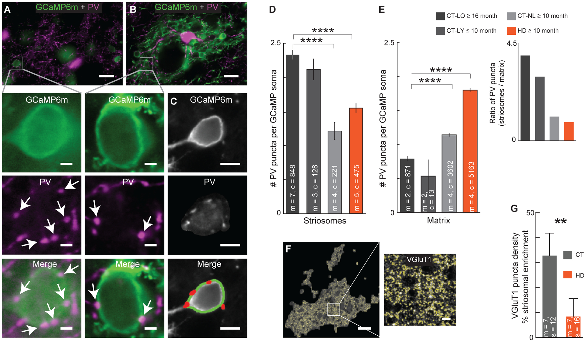
(A-C) Peri-somatic PV puncta (pink) in striosomes (A) and matrix (B) by detection of GCaMP6m-labeled cell bodies (green), and PV puncta (red) by automated image analysis (C). Scale bars, 20 μm (A and B), 2 μm (inserts for A and B), and 5 μm (C).
(D and E) PV puncta on GCaMP6+ cell bodies (c, mean ± SEM) were reduced in striosomes (D) and increased in matrix (E) in both CT-NL and HD mice (****p < 0.0001, Kruskal-Wallis and Dunn’s multiple comparison test). The number of PV puncta was greater in striosomes than in matrix in CT-L mice (p < 0.0001, two-sample t-test). Striosome-to-matrix PV puncta ratio was greater than 1 in CT-L mice (insert).
(F) VGluT1 puncta detected (yellow) in a striosome. Scale bars, 50 μm, 5 μm (insert).
(G) Striosomal enrichment of VGluT1 puncta density, relative to matrix, was significantly higher in CT than in HD brain sections (**p = 0.0087, Mann-Whitney test).
We also investigated putative excitatory corticostriatal inputs to striosomes in CT and HD mice by immunostaining for VGluT1. In the CT mice, VGluT1 puncta density was significantly higher in striosomes than in matrix, and this striosomal enrichment was reduced in HD mice by ~23% along with VGluT1 puncta intensity in both striosome and matrix compartments (Figures 6F, 6G, and S6D–S6H). We also found lower dendritic spine density on striosomal, but not matrix, SPNs in HD compared with CT mice (Figures S6I–S6N), a finding that could not be attributed to reduced cross-sectional area in HD mice (Figure S6O) or to differences in D1 and D2 spine density in CT mice (Figure S6P).
Of these measures of excitatory and inhibitory circuit connectivity markers, putative PV- sSPN connection number was the only measure found to be correlated with R−CRP activity in both CT and HD mice (Figures S6Q–S6S). These findings point to a disconnection of striosomal circuits, but not of matrix circuits, in HD model mice as well as in CT-NL mice, and suggest that inhibitory input to striosomes from PV neurons could serve as an important mediator of learning. Future work is required to consider whether other sources of inhibition, such as interneuronal subtypes, SPN collaterals or even glial cells, are involved (Khakh, 2019).
Difference in Compartment-Specific Functional Connectivity between Striatal Fast-Spiking Interneurons and SPNs
To examine compartment-specific functional connectivity between striatal FSIs (putative PV interneurons) and putative SPNs, we turned to rats, with their larger brain size, to perform simultaneous electrophysiological recordings from FSIs and SPNs. We were able to record with high temporal resolution 38 putative FSI-sSPN pairs, 76 putative FSI-matrix SPN (mSPN) pairs, and 7 FSI-sSPN-mSPN triplets across 8 rats, which required recording from 14,785 well-isolated neuronal units (STAR Methods). We found strikingly different modulation of sSPNs and mSPNs studied out of task (Figure 7A–7F). In striosomes, FSIs modulated SPNs by decreasing SPN activity with a graded slope, whereas in matrix, the modulation was a sharp step-function. This surprising finding led us to speculate that sSPNs were contacted by multiple putative PV+ terminals, potentially allowing a greater range in the levels of inhibition exerted by FSIs onto sSPNs than mSPNs (Figures 6D, 6E, 7E, and 7F). In other words, activation of one terminal could result in a low level of inhibition, whereas activation in multiple terminals might result in higher levels of inhibition. This anatomical pattern might underlie the graded decay response observed in FSI-sSPN pairs.
Figure 7. FSI-Striosomal Functional Connectivity Supports Model of PV Role in Striosome-Mediated Discrimination Learning.
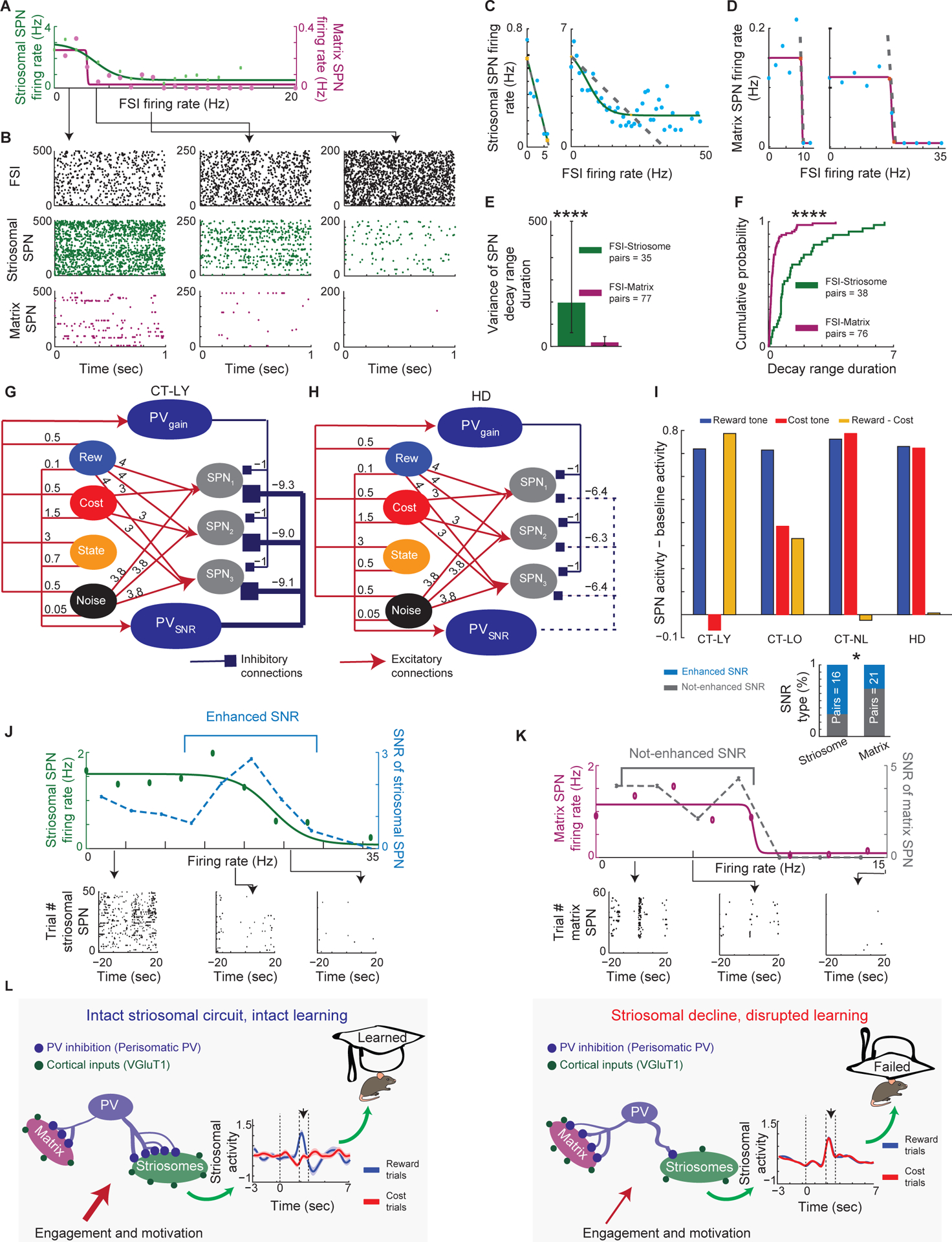
(A and B) Firing rates of simultaneously recorded sSPNs and mSPNs as functions of FSI firing rate (A) and their raster plots (B) during periods of low (left: 0–2 Hz), medium (middle: 3–4 Hz), and high (right: 7–10 Hz) FSI firing rates.
(C and D) Sigmoidal function fitted to striosomal (C, two examples) and matrix (D, two examples) SPN firing rates as functions of FSI firing rates. In the middle portion of each sigmoid, SPN firing decayed as FSI firing increased (dashed gray line).
(E) Decay ranges were more variable for FSI-sSPN than FSI-mSPN pairs (variance ± confidence interval for variance, F-test, ****p < 0.0001).
(F) Decay ranges were longer for FSI-sSPN than FSI-mSPN pairs (K-S test, ****p < 0.0001).
(G and H) Probabilistic spiking network models constructed based on our histological observations from Figure 6. A neuron’s probability of firing was determined by a sigmoidal output function. Numbers above arrows show connection strengths. Reward (blue) and Cost (red) neurons inputted trial-type information. Noise neuron injected noise (black). State neuron (orange) controlled engaged and not engaged states. Input was a firing pattern of Boolean values, where the Noise neuron fired with probability 0.95. In reward trials, the Reward neuron fired, and Cost neuron did not; in cost trials, both neurons fired. We measured model output activity by averge number of activated SPNs per trial. Only connections between PVSNR and SPNs were different across the groups and provided strong inhibition in CT-LY (G), weak inhibition in CT-LO (Figure S6A), and even weaker in HD (H) and CT-NL (Figure S6B) mice. Connectivity ranges were estimated based on Figure S7C.
(I) Output activity of trained model SPNs (averaged from 10000 trials) reached observed target photometric activity in each group (compare to average striosomal activity in Figures 4A and 5D). To evaluate relative activation of model sSPNs for cost and reward signals, we subtracted baseline activity computed by initiating the model only with noise input from model output.
(J) An example of FSI-striosomal connectivity in which FSIs modulate SNR of sSPN activity (STAR Methods), with SPN raster plots for low (0–3.8 Hz), medium (15.2–19 Hz), and high (22.8–26.6Hz) FSI activity (bottom). As the SPN firing rate decreases due to increasing FSI activity, SNR first increases then decreases (top). This suggests that when the peak of SNR is in the middle of the decay range of sSPNs, FSIs not only inhibit sSPNs, but also enhance SNR.
(K) Same as J, but for FSI-matrix connectivity in which FSIs modulate mSPN activity in a decay-like manner (top), with SPN raster plots for low (0–4 Hz), medium (4–8 Hz), and high (12–16 Hz) FSI activity (bottom). Comparison of FSI-striosomal and FSI-matrix pairs showed that SNR was enhanced more in sSPN than mSPNs (insert; chi-square test, *p = 0.032).
(L) Summary of the findings. In mice that learned, levels of excitatory cortico-striosomal and inhibitory PV-striosomal connectivity together with discriminative striosomal signals were high (left). In mice that failed to learn and in HD mice, circuit connectivity level was low, and discriminative striosomal signals were absent. Green dots: excitatory cortical inputs onto SPN dendrites; blue lines: peri-somatic PV inputs onto SPN cell bodies.
Modeling of PV-Striosomal Connection to Test for Plausible Links between Striosomal Activity and Striosomal Circuit Architecture
To test the hypothesis that PV-striosomal functional connectivity is important for discrimination learning, we developed a model linking striosomal activity and histological measures. Our main hypothesis was that varying connection strengths between PV neurons and sSPNs could produce the difference in striosomal R−CRP across different groups of mice. A decay of PV-SPN connectivity in striosomes might therefore disrupt the development of learning-related striosomal signals. We implemented a stochastic spiking neural network model and designed models of CT-LY, CT-LO, CT-NL, and HD mice (Figures 7G, 7H, S7A, and S7B). We constructed these models to replicate the average R−CRP across groups (Figures 7I, S7C, and S7D) in which task information was represented by inputs reflecting reward tone, cost tone, noise and task engagement. In HD and CT-NL models, given PV→SPN constraints in our network architecture, weights of other elements representing cortical inputs could not be optimized to reach best-performing group discrimination levels shown by CT-LY mice, as measured by the error between photometrically observed and modeled activity outputs (Figure S7E).
We then hypothesized that PV neurons could potentially contribute direct inhibition during cost trials, resulting in increased SNR in sSPNs, thereby improving stimulus selectivity alongside modulation of SPN gain. We hypothesize that in an “engaged” state, this architecture would result in enhanced performance, an aspect of the model represented by way of a “state” neuron. This increase of inhibitory currents would result in noise signals being unable to overcome striatal inhibition, whereas more strongly connected task signals would be capable of doing so, resulting in an improved SNR. The model thus posits that additional inhibition during performance will improve discrimination and decrease noise (Figure S7F).
Our model suggested that PV neurons modulate striosomal SNR. Thus, we asked whether this phenomenon might indeed be plausible in striosomal microcircuits. We developed two analyses to measure how SNR is modulated by FSI activity. We demonstrated that the FSI-induced decrease in sSPN activity could be modeled as enhanced SNR. In matrix, decaying SPN activity could be modeled as decaying SNR (Figures 7J, 7K, S7G, and S7H). We speculate that FSI-striosomal functional connectivity, by way of SNR modulation, could serve as a ‘filter’ of cortical activity, allowing selective signal passage. By contrast, FSI-matrix functional connectivity could serve solely as a ‘gain’ modulator of incoming signals to striatum, diminishing all signals. This finding is in accord of our observation that SNR increased in recordings of Ca++ transients across learning in striosomes but not in matrix (Figure S2P). Therefore, the observed capacity of FSIs to modulate striosomal SNR may be critical to the process of valence-based discrimination learning.
DISCUSSION
Our findings suggest that the striosome compartment of striatum, here examined in its anterior part (DMS), is critical for valence-based learning. We found a strong correlation between population activity of striosomal SPNs and successful valence-associated discrimination. These signals and correlations were sensitive to motivational value as tested by outcome devaluation. Chemogenetic manipulation of striosomal circuits produced shifts in the engaged state that modulates learning. In sharp contrast to these findings for striosomes, we did not observe such correlated activity patterns or motivational sensitivities for the populations of mSPNs examined with the same methods. Selective dysfunction of striosomal neurons was accompanied by an inability to achieve valence-based learning, whether these problems were induced by age or modeled HD status. Our work further demonstrates striking compartmental differences in functional and local circuit connectivity of striosomes and surrounding matrix. We hypothesize that such targeted microcircuits including putative PV-striosome circuits control SNR of sSPN firing by filtering out noise during the process of learning (Figure 7L).
Striosomes Could Serve as a Subjective Value Filter via Integration of Cortical Task Information and Engagement State
Regions of frontal neocortex, including specific regions of anterior cingulate and orbitofrontal cortex, preferentially project to striosomes (Donoghue and Herkenham, 1986; Eblen and Graybiel, 1995). In many of these regions, value-related signals have been recorded (e.g., Amemori and Graybiel, 2012; Padoa-Schioppa and Assad, 2006; Schoenbaum et al., 2009; Wallis, 2011). As we show here, striosomal activity increases or decreases with expected value and is sensitive to engagement and motivational states. Direct chemogenetic excitation or inhibition of striosomal populations shifted behavioral expression of motivational state. Based on our findings, we speculate that striosomes integrate engagement states and expected value signaling, which together could reflect subjective value on the path toward learning. Striosomes are considered to be the main source of direct projections from striatum to midbrain dopamine-containing neurons in SNpc, which, in turn, are a major source of dopaminergic projections to striatum. Our findings suggest that this striosomal targeting of SNpc neurons could contribute to shaping value-based parameters attributed to midbrain dopamine neuron signaling (Cohen et al., 2012; Kawagoe et al., 1998; Lak et al., 2014; Schultz, 2017).
Difference between Striosomes and Matrix in Experience-Dependent Plasticity
During learning, Ca++ transients in striosomal populations that we recorded decreased in frequency and showed a trend toward increasing amplitude. This pattern is consistent with the possibility that, as learning occurs, striosome-based circuitry undergoes refinement via plasticity mechanisms (Harada et al., 2019; Owen et al., 2018; Xiong et al., 2015; Znamenskiy and Zador, 2013). We note here that given the slow time-course of GCaMP6m signaling, the frequency and amplitude of Ca++ transients might together reflect the development of more synchronized or patterned spike activity indicated by increased SNR. Work in slice preparations suggests that striosomal neurons are differentially sensitive to dopamine and are more excitable than neurons of surrounding matrix (Prager and Plotkin, 2019), a difference that we also see in our electrophysiology recordings reported here. These features of higher excitability coupled with dopamine sensitivity could promote differential striosomal circuit refinement by plasticity mechanisms relative to those of matrix circuits.
Physiological Function of the Matrix Compartment
Unlike striosomal activity, activity in matrix did not change in correlation with discrimination. Instead, the matrix signals recorded were correlated specifically with reward-trial RP lick rates, yet not cost-trial or reward consummatory licks in single sessions, indicating that the matrix signals do not simply reflect motor lick rates. This pattern is reminiscent of neuronal representations encoding higher levels of abstraction, such as chunked behavioral units, rather than simple movements (Graybiel, 1998; Martiros et al., 2018). These observations could indicate that activity in matrix, as reported for striatum in general (e.g., Samejima et al., 2005), reflects action value, given that lick rates in reward trials scaled with value. When we looked for devaluation sensitivity in matrix signals, we found that they, unlike the striosome signals, were not susceptible to reward devaluation, and that they were not correlated with the degree of task engagement. Striosomes, as identified in our ‘striosome mice’, integrated both reward-related and cost-related values, as well as motivation-related influences, with the result that they encoded a comprehensive subjective value signal about the impending outcome.
Computational Role of PV Neurons in Reducing Noise Affecting Discrimination Learning
We developed a graph-based model by which PV interneurons exerting inhibition onto striosomal neurons could improve discrimination through shifting excitation-inhibition balance (van Vreeswijk and Sompolinsky, 1996; Vogels and Abbott, 2009) due to modulating SNR alongside gain (Atallah et al., 2012; Carandini and Heeger, 1994; Carandini et al., 1997; Kvitsiani et al., 2013; Wilson et al., 2012). In FSI-sSPN pairs, we found enhanced SNR with increased FSI firing rate, suggesting that this connection could function as a filter by which weak signals are suppressed as noise and stronger signals pass. This filtering would result in a relative SNR increase, even while inhibition is driving down overall activity. By contrast, in FSI-mSPN pairs, increased FSI firing rate drove down SPN ‘signal’ and ‘noise’ without enhancing SNR of activity, in a simple modulation of gain. Critically, our results suggest that minor differences in network composition can translate to a circuit’s function, whether this composition encodes SNR or gain.
Learning from Cost vs. Learning from Reward: Two Striosomal Loops with the Dopamine System
To our surprise, HD mice were more likely to exhibit cost-related learning than reward-related learning, in marked contrast to signaling in CT mice. A working hypothesis is that this phenomenon could reflect an abnormality in striosomal encoding of influence on both cost and benefit signals conveyed by striosomal downstream projections to both the dopamine-containing neurons of the SNpc (Crittenden et al., 2016; Evans et al., 2019; Fujiyama et al., 2011; McGregor et al., 2019) and the LHb (e.g., Hong et al., 2019), known to have neurons that can be excited by unrewarding options and to inhibit dopaminergic neurons (e.g., Hikosaka, 2010). Thus striosomes, by virtue of their input to these two circuits, could influence state-dependent modulation of dopaminergic neurons (Figure S7I). If the function of the striosome-SNpc circuit is degraded, as in neurodegenerative HD patients, the striosome-LHb-SNpc pathway might then prevail, facilitating learning from cost as observed in psychiatric disorders (Jean-Richard-Dit-Bressel et al., 2018). This circuit balance, itself dynamic, could participate, in coordination with other circuits, in shifts in decision-making and learning strategies that have been observed in aging, in HD and in other neurodegenerative disorders (Eppinger et al., 2011; Gleichgerrcht et al., 2010; Strough et al., 2015). We appreciate that other circuit modifications could as well affect such balancing of circuit function.
Striatal Microcircuit Degradation in Human HD Versus HD Mouse Models
In human HD patients, indirect (D2) pathway degeneration has classically been interpreted to prevail earlier followed by direct (D1) pathway decline (Glass et al., 2000; Reiner et al., 1988; Richfield et al., 1995a; Richfield et al., 1995b), whereas in mouse studies earlier degeneration in D1 SPNs has been observed (Goodliffe et al., 2018). In these early studies, human HD tissue was evaluated without reference to striatal compartmentalization, but with markers such as substance P and endocannabinoid receptor, CB1, which tend to show enriched expression in the striosomal compartment. In HD model mice, we observed spine density decreases selectively in striosomes, but, consistent with other work (Deng et al., 2013), VGluT1 levels decreased more generally across compartments. This dual pattern is in accord with earlier work on human HD tissue in which general loss was observed across striatum, even when augmented loss was observed in striosomes (Tippett et al., 2007). This parallel raises the interesting possibility that our findings along with those of prior studies in mouse and human could potentially find agreement in declines in striosomal circuits in HD.
We discuss limitations of the study in STAR Methods (Limitations of This Study and Issues for Further Work). Despite these, the differences that we have found between putative striosomal and matrix signals suggest that this compartmentalization of the striatum has profound effects on the differential control of valence-based learning and decision-making and their vulnerability across aging and neurodegenerative disease.
STAR Methods
RESOURCE AVAILABILITY
Lead Contact
Further information and requests for data and reagents should be directed to and will be fulfilled by the Lead Contact, Ann M. Graybiel (graybiel@mit.edu)
Materials Availability
This study did not generate new unique reagents.
Data and Code Availability
The published article includes all datasets and code generated or analyzed during this study.
Datasets generated during this study are available at Mendeley at http://dx.doi.org/10.17632/6z4fvrspt3.1, http://dx.doi.org/10.17632/6r6d39rs7j.1, and http://dx.doi.org/10.17632/3xdtk8gdbd.1.
Code generated for this study have been deposited at github at https://github.com/sdrammis/Friedman-Hueske-2020/tree/v1.0.2.
Details on the use of the code for the processing of the raw data are found in the Supplemental file, Data S1.
EXPERIMENTAL MODEL AND SUBJECT DETAILS
All mouse colonies were maintained in accordance with the policy at the Massachusetts Institute of Technology (MIT) and the U.S. National Research Council Guide for the Care and Use of Laboratory Animals. All experimental procedures were approved by the Committee on Animal Care at MIT. All mice were kept under constant temperature (25°C) and humidity (50%), and a 12:12 hr light/dark cycle. Mice were housed 2–5 per cage unless experimentally implanted in which they were housed individually. All mice were housed in an enriched environment with ecobedding, nestlets and PVC tube cylinders. All experiments were conducted using mice of age ranges specified or, for birthdate breeding, dosed according to developmental stages as described. All experiments included roughly equal male and female subjects randomly assigned. No influence of sex was found on the results reported in this study.
Transgenic Mice
The following mouse strains were used for behavioral, neural recording and histological experiments: Mash1-CreER (Kim et al., 2011), Dlx1-CreER (Taniguchi et al., 2011), Ai14 (Madisen et al., 2010), LSL-Flpo (He et al., 2016) and Q175z knock-in (KI) mice (Menalled et al., 2012). To evaluate proportions of D1- and D2-type neurons labeled by this method at striosomal and matrix timepoints, the following mouse strains were used: Mash1-CreER or Dlx1-CreER mice crossed with Ai14 were mice backcrossed in-house and maintained on an FVB background corrected for behavioral optimization. Mouse lines targeting striosomal and matrix cell populations were generated according to inducible genetic fate-mapping procedures previously described (Kelly et al., 2018). We crossed either Dlx1-CreER or Mash1-CreER mice to the Cre-dependent LSL-Flpo on an FVB background corrected for behavioral optimization. Subsequently, by crossing female Dlx1-CreER;LSL-Flpo or Mash1-CreER;LSL-Flpo mice with male heterozygous Q175z KI mice on a C57BL/6J background, F1 hybrid mice were produced to better suit behavioral characterization (Menalled et al., 2014). Upon observing a vaginal plug, noon of that day was counted as embryonic day 0.5 (E0.5), and tamoxifen was administered by gavage to the pregnant female at E10.5–11.5 to achieve striosomal Flp expression or E15 to achieve matrix Flp expression (Taniguchi et al., 2011). To reduce disruption to pregnant females by estrogenic effects of tamoxifen, females were co-administered progesterone (tamoxifen and progesterone dissolved in corn oil by gentle agitation for 24 hr), using a 20-gauge 33-mm gavage tool at a dose of 100 mg/kg body weight determined empirically to maximize expression while maintaining dam and pup health. For evaluations of proportion of D1R- and D2R-expressing cells targeted in each cross and Cre-induction timepoint, Dlx1-CreER;Ai14 or Mash1-CreER;LSL-Flpo mice were crossed with D1-eGFP and D2-eGFP mice (Gong et al., 2007); tamoxifen was administered at E11 or E15 for each cross.
Limitations of This Study and Issues for Further Work
Our tamoxifen-dependent birthdate-labeling approach only labeled a minority of striosomal neurons (Bloem et al., 2017; Kelly et al., 2018). Further, in ~E11 born striosomal cell populations, we observed a bias toward D1 SPNs, and, in the ~E15 born matrix neurons, there was a bias toward D2-expressing SPNs (Kelly et al., 2018; Tinterri et al., 2018). However, it has been demonstrated that in some regions of striatum, striosomes are highly D1 biased and matrix are D2 biased (Miyamoto et al., 2018). Additionally, whereas we observed that spine density in the zQ175 HD model mouse was selectively reduced in striosomes, other studies suggest more widespread decreases in spine density (Indersmitten et al., 2015) or decreases selective to D1 SPNs (Goodliffe et al., 2018). In contrast to our own measurements in anterior DMS, these reports were based on counts for the dorsolateral striatum. Given the gradients of D1 and D2 and other neurochemicals and intraneuronal circuits (Cox and Witten, 2019; Miyamoto et al., 2018; Stalnaker et al., 2010; Voorn et al., 2004), and the variety of differences across HD models (Donzis et al., 2019), an intersectional approach to evaluate both D1 and D2 SPN populations in striosome and matrix compartments could help in clarifying these issues.
A further concern is that the numbers of striosomal and matrix cells that contributed to population Ca++ photometric signals were different. However, we observed clear transients across different task conditions for both striosome and matrix mice, and in the striosome mice, but not the matrix mice, DREADD manipulations altered engagement.
We examined only putative PV interneurons, and did not examine other interneuronal cell types, including somatostatin+ neurons (e.g., Gittis and Kreitzer, 2012; Holly et al., 2019), astrocytes (Wojtowicz et al., 2013), or even recursive collaterals directly emanating from striatal SPNs (Tepper et al., 2008), which might contribute to the findings that we report here.
Engagement state could reflect mechanisms not studied here, including reduced dopaminergic or other aminergic signaling (Kanazawa et al., 1993), cholinergic activity, and/or reduced thalamic attentional gating mechanisms as seen in model HD mice (Deng et al., 2014) and in HD patients (Finke et al., 2006).
Despite these limitations, the differences we found between striosomal and matrix signals suggest that the compartmentalization of striatum has profound effects on the differential control of valence-based learning and decision-making across aging and HD.
Details of Water Restriction
To preserve the health of aged HD and control mice, daily HydroGel (ClearH2O, Portland, ME) was provided to bring session-obtained water to approximately 2 ml of water per day (1.7–2.7 depending on mouse body condition). Mice were maintained at >90% body weight with free access to food. Mice had free access to water on weekends and resumed water restriction 12 hr before the next session. For DREADD experiments, mice continued water restriction over weekends to reduce day-of-week effects.
METHOD DETAILS
Surgery Procedure
Prior to surgery, mice were injected with meloxicam as a pre-surgical analgesic at 3 mg/kg (IP) and for 3 days post-surgically as needed at 1 mg/kg. Mice were anesthetized with 3% isoflurane and were maintained under anesthesia with 1–2% isoflurane. Antibiotic ointment was applied to the incision once a day, and 0.5 ml of Ringer’s solution was administered (IP) for three post-surgical days, including the day of surgery. These extra measures were taken to ensure the health of aged HD and control mice.
For surgical coordinates and details of chemogenetic manipulation experiments, see ‘DREADD with Photometry Experiments.’ For photometry recordings during behavior, mice were injected bilaterally with AAV8-Ef1a-fDIO-GCaMP6m (Stanford Vector Core) targeting anterior central dorsal striatum. To achieve this location across a range of aged mice in our mouse strain, coordinates were determined empirically according to the following: Intended atlas coordinates for virus injection based on 26–30 g C56BL/6J mouse (Paxinos and Franklin, 2001) were AP +1.1 mm from bregma; ML ±1.25 mm; DV −2.0 mm from brain surface. Intended implant atlas coordinates were AP: +1.1 mm from bregma; ML: ±1.25mm; DV: −2.1mm from brain surface.
Empirically determined coordinates for aged F1 hybrid background birthdate-labeled mice were as follows:
Bilateral viral injections of 500 nl volume:
for age 6 months: AP: +1.1 mm; ML: ±1.5 mm; DV: −2.0 mm from brain surface
for age 9 months: AP: +1.3 mm; ML: ±1.5 mm; DV: −2.0 mm
for age >12 months: AP: +1.6 mm; ML: ±1.5 mm; DV: −2.0 mm
Unilateral fiber implant:
for age 6 months: AP: +1.1 mm; ML: ±1.5 mm; DV: −2.1 mm from brain surface
for age 9 months: AP: +1.3 mm; ML: ±1.5 mm; DV: −2.1 mm
for age >12 months: AP: +1.6 mm; ML: ±1.5 mm; DV: −2.1 mm
Injections were performed using a 33-gauge needle attached to a Hamilton syringe at a rate of 0.1 μl/min. After each injection, the injection needle remained in place for 8–10 min to allow full dispersion of the virus. Once the virus was injected, we allowed 4 weeks before implantation of optical fibers (Doric Lenses, MFC_400/430–0.48_5mm_MF1.25_FLT). In order to aid fiber penetration of brain tissue, a 23-gauge needle was lowered to the injection site. The optical fiber was implanted at 100 nm ventral to injection coordinates. Each fiber was tested to ensure more than 95% efficiency in advance of implant. A head-bar was cemented to the animal’s skull 8 mm to 10 mm posterior from the bregma for the head-fix apparatus. Recordings during behavioral tasks began 2–4 weeks after fiber implants.
Apparatus
In order to train mice on a discrimination learning task while performing photometry imaging, we designed and built a custom-developed Arduino-controlled (Adafruit 50) head-fixed behavioral apparatus. The apparatus was comprised of 3D-printed components including a retractable lick spout for liquid reward delivery and a semi-circular panel of LEDs (super bright blue; Adafruit 301) for delivery of varying intensities of light as aversive outcome. Components were assembled on an aluminum breadboard (ThorLabs MB6) with optical posts (ThorLabs TR4-P5 and TR3-P5). Sound isolation chambers were constructed from acrylic board and acoustic foam (McMaster-Carr 9710T11) in order to buffer auditory stimuli delivered inside by standard speakers. Mice were head-fixed using a custom-made head-bar, with their body held inside a PVC tube with forepaws placed on a foot pedestal. In order to provide liquid reward, a servo (Sparkfun 09065) allowed positioning of the lick spout in front of the snout of the mouse during response and outcome periods, which allowed retraction of the lick spout during the inter-trial interval (ITI) and tone periods. The lick-spout start position was aligned at the beginning of the experiment to allow for accurate detection of licks by the embedded lickometer using an infrared emitter-detector set (Sparkfun 00241) and consumption of delivered liquid rewards (Parker Hannifin 003-0260-900). The number of licks during the response period was measured by IR beam breaks at the lickometer. A speaker (iHome iM70BC) was positioned inside the sound isolation chamber to deliver auditory stimuli. Behavioral protocols were administered using an arduino-based microcontroller wired through a custom-designed printed circuit board (https://github.com/sdrammis/Friedman-Hueske-2020/tree/v1.0.1/circuit_arduino-hardware_behavior_apparatus). In order to record the timestamp and identity of task events, the Arduino microcontroller was connected to a PC using serial port, and the data were acquired using a custom-developed Python program described in Data S1 section ‘Codes for Photometry and Behavior Data Acquisition’.
Approach-Avoidance Behavioral Assays
Acclimation
In order to acclimate the mice to the environment of the head-fix apparatus, mice were housed with the PVC tube used for head-fixing in their home cages a week before the start of training. On the first two days, mice were placed in the head-fix apparatus for half an hour.
Approach-Avoidance Discrimination Task
Each daily behavioral training session on a discrimination task consisted of a maximum of 150 trials, comprised of randomly interleaved reward and cost trials. The trial structure had a sequence of four events: an auditory tone (2 s, 4 or 8 kHz) signifying a reward and cost trial (or vice versa), a 1-s response period (abbreviated as RP in main text) in which a lick spout became available and response licks were measured using a lickometer, an outcome period in which either 10% sucrose drops (4 μl) were delivered from the lick spout during reward trials or, in the case of cost trials, a semi-circular LED positioned around the head of the mouse delivered light at 4–400 lux. The number of licks during the response period determined the magnitude of reward or cost delivery in the outcome period. Reward and cost were implemented as the number of sucrose drops delivered from the lick spout, and the delivery of LED light, respectively, such that <3 licks resulted in 1 drop of sucrose or 4-lux light, 3–4 licks in 3 drops of sucrose or 40-lux light, and >4 licks in 6 drops of sucrose or 400-lux light. An ITI (6–14 s) followed the outcome period before the next trial.
Performance Criterion
In order to determine when a mouse learned a task, we compared distributions of response-period (RP) lick rates for reward and cost trials. In order to have enough trials to calculate and compare lick-rate distributions, we collected data from two consecutive sessions and calculated the significance of the difference in cumulative distribution functions (CDF) of response-period licks between reward and cost trials using a Kolmogorov-Smirnov test (K-S test). We determined that each mouse learned a task when there was a significant difference in two consecutive K-S tests. Since each K-S test was performed on data from two consecutive days, the significance was determined by sessions spanning three days; the first significant K-S test was based on days 1 and 2, and the second K-S test was based on days 2 and 3. All mice participated in the analysis without exclusion criteria. For K-S test analysis functions, see Data S1 section ‘Performance Criterion Functions’.
Reversal of Cue-Outcome Contingencies
Once a mouse reached the performance criterion of learning the original cue-outcome associations in the discrimination task, these contingencies were reversed, and the mouse was trained until the performance criterion was met again for the reversal learning.
Reward Devaluation
In order to assess hedonic processing, we devalued the rewarding outcome by providing mice free access to sucrose or water for 1 hr prior to a session of the discrimination task. We evaluated the response after free access to sucrose or water to determine the development of a habit as a conditioned response to the stimulus or decline in response based on satiety or reduction in seeking reward.
Enhancing Cost-Tolerance
In order to evaluate the effects on behavior and striatal compartment function of an anxiolytic, which is thought to increase cost-tolerance, mice were dosed with diazepam (0.5 mg/kg, IP) or saline 10 min prior to the beginning of a session of the discrimination task.
Control Tasks
Subsets of mice were tested in a battery of control tasks that took place in an approximately balanced manner before or after training on the discrimination task.
Light Avoidance
To assess whether the aged and HD mice perceived and showed equivalent aversion to light, we ran the mice through a 6-day protocol to observe light avoidance tendency. Mice were habituated to TruScan activity monitor chambers (Coulbourn Instruments, Whitehall, PA) over 5 days (2 days with a 15-min period and 3 days with a 1-hr period, also used to assess locomotor activity) before starting light aversion testing. A black acrylic chamber divider separated a dark side from a side bathed in white LED light with a door at the center. In the bright compartment, the light was calibrated to 4, 40, or 400 lux. Mice were initially placed into the dark side of the box and then allowed to move between the dark and light compartments for 5 min. Boxes were cleaned between sessions. All mice completed the light-avoidance task battery in the following order: 4 lux, 40 lux, and 400 lux. Lights remained constant on one side of the box, and mice were moved between boxes to alternate which side was bright. Mice were balanced for whether they ran this task before or after training, and for left-right location of the light in the chamber. Mice spent significantly less time on the lit chamber side with increasing light levels (Figure S4R).
Sucrose Preference
To assess whether HD mice differed from control mice in reward preference for sucrose, mice were put into a fresh cage with two bottles containing 10% sucrose solution and water. They were given free access to the two bottles over a 4-hr period, and bottles were weighed before and after the session. Mice were tested in a water-restricted state or normal state, and the test was performed once before locomotor/light aversion testing and once after.
Pupil Diameter Measurement
As a supplementary way to estimate the states of arousal, we measured pupil diameter during the discrimination task. During the task, a camera that could take images under infrared light (Sparkfun 11610) captured an image using a microcontroller (Arduino Uno) when the TTL pulse was sent from the Arduino controlling the multi-color multi-fiber photometry system to the camera. The microcontroller also kept an 850-nm LED (Sparkfun 09469) on during recording. To ensure no movement during recording, the camera along with two magnifying lenses were mounted to an optical post. We put the lenses directly in front of the camera, and placed the lens close to the eye (15 cm away). In order to reduce glare, the 850-nm LED was set to the side of the mouse’s camera 10 cm away. The images were stored to a micro SD card (Samsung MB-ME256GA/AM) via a micro SD card shield (Sparkfun 1276) attached to the microcontroller. See Figure S1H.
Multi-Color Multi-Fiber Photometry System
To capture the brain activity in five mice simultaneously, we developed a five-fiber photometry system (Kim et al., 2017), interleaving blue (470 nm) LED light to activate GCaMP and purple (405 nm) LED light as a control (Figure S2D). We delivered the LED light into the brains of individual mice with a custom-made five-fiber patch cord (Doric Lenses) and recorded signals from each mouse with a sCMOS camera (Hamamatsu, ORCA-Flash4.0). With HCImage Live and functions custom-written in Matlab (Mathworks), we captured 512 × 512 images and selected regions of interest for each fiber. In order to easily adjust and align each component, we used Thorlabs optomechanical products.
Optical Elements for Photometry System
To ensure both the 405-nm and 470-nm LED lights reached each brain, and the successful recording of GCaMP signal, we used a series of dichroic mirrors and filters. To first focus the 470-nm and 405-nm light, we passed both lights through a fiber collimation package (F240SMA-A, Thorlabs). Afterwards, the 470-nm and 405-nm light were filtered using Thorlabs, MF469–35 and Thorlabs, FB405–10. In order to combine both lights into one beam, we used a 425-nm long-pass dichroic mirror (Thorlabs, DMLP425R) to reflect the 405-nm light into the same beam as the 470-nm light. In order to allow the 470-nm and 405-nm light to reach the brain target and the return GCaMP signal to the camera, we used a 495-nm edge BrightLine® single-edge dichroic beamsplitter (Semrock, FF495-Di03–25x36). The 470-nm and 405-nm light passed through the 495-nm dichroic beamsplitter and focused into the five-fiber bundle by a 20×/0.75-NA objective (Nikon, CFI Plan Apo Lambda 20×). The GCaMP signal from each brain was picked up by the fiber bundle, magnified by the 20×/0.75-NA objective, and passed through the 495-nm dichroic beamsplitter. The fiber bundle was connected to each mouse with a zirconia sleeve (Doric Lenses, SLEEVE_ZR_1.25). To filter the GCaMP signal, we passed it through a 525-nm emission filter (Thorlabs, MF525–39). To further focus the fiber bundle image onto the camera, we focused the light with an adjustable lens in rotating housing (Thorlabs, SM1NR1). For more details see Figure S2D and resource table.
Photometric System Validation and Signal Verification
To avoid autofluorescence and cross-talk between the fibers, we used custom-made optical fibers from Doric Lenses. We requested fibers that used low autofluorescence epoxy, and cladding around each fiber to disrupt cross-talk.
There were multiple tests for the system. Test 1 was designed to ensure that there was no cross-talk between the bundled fibers. We placed the end of one of the five fibers into a beam trap (Thorlabs, BT600/M) and shined 10 kLux light through all of the remaining fibers. We then measured, using a camera, light intensity from the bundled five fibers. We verified that the value of light from the trapped fiber was below 200 when the value from the other four fibers was around 65,000 in a camera with dynamic range of 100–65,353. Test 2 was performed to ensure that the autofluorescence of the entire system was minimal. While the 470-nm LED lights were on, we ensured that there was no reading of more than 1800 by the camera. Otherwise, the fiber cable was bleached using 470-nm laser for 24 hr. In order to have equivalent excitation and control light to each mouse, we adjusted the optics so that each fiber was within a 10% range in μWs of LED light. The connection between the fiber bundle and the implant was also measured so that each implant had at least 90% yield. To ensure optimal SNR of the system, we tested striosome-expressing GCaMP6m mice with different intensities of the 470-nm and 405-nm light. We found that 100 μW of 470-nm light and 65 μW of 405-nm light, with an exposure time of 53 ms, were ideal.
Microcontroller System to Drive LEDs and Camera
To control and synchronize the LEDs and camera, we used a microcontroller (Arduino, Arduino Uno Rev3). In cycles of 66 ms, we programmed the microcontroller to alternate between the 470-nm light and 405-nm light. Each time an LED was turned on, the microcontroller signaled the camera to capture a frame. Through the HCImage Live software, we controlled the exposure time to 53 ms to ensure the camera captured only while the LED light was on. To avoid exposure overlap, we included a 13-ms delay after each frame. In order to synchronize the frames captured with our behavioral system (see below), our program for the microcontroller also sent a TTL pulse after every 200 frames to each of the behavioral apparatuses.
Temporal Synchronization with Behavioral Apparatuses
To ensure that the behavioral recordings and photometry frames were synchronized in terms of their internal clocks, we measured the jitter of each and aligned according to TTL interrupts to realign the recordings.
Acquiring and Digitizing GCaMP Emission in Photometric System
In order to image the GCaMP emission signal, we used a digital sCMOS camera (Hamamatsu, orca flash 4.0 v2) to record 512 × 512 pixel images, with a 4 × 4 binning readout, and a pixel size of 6.5 μm × 6.5 μm. Each region of interest, i.e., each fiber, was approximately 175 × 175 pixels. To avoid dropped frames, we first saved the recordings to RAM, and to ensure precise time measurements for synchronization, we recorded in CXD file format. To distinguish between each fiber, we applied five regions of interest using functions custom-written in Matlab. To decipher signals from 470-nm light excitation compared to the baseline 405-nm light, we extracted signal from frames taken during 470-nm and 405-nm exposures separately. For phometric preprocessing and extraction codes, see Data S1 section ‘Photometry Recording Preprocessing.’
Calcium Transients Extraction and 405-nm and 470-nm Comparison
To extract, isolate, characterize, and validate transients, we created a custom-designed algorithm (see Data S1 section ‘Calcium Recordings Transient Extraction and Signal-to-Noise Ratio Codes’). We began our analysis by removing artifacts that came from animals’ movements or rare large disturbances of the system. We then determined which function among one-degree polynomial, two-degree polynomial, one-degree exponential, and two-degree exponential best fitted the regression trend caused by GCaMP bleaching. We then subtracted the best fit function to remove the trend. After these cleaning steps, we converted the 405-nm and 470-nm channel signals to z-scores. In order to find exact transient start and peak times and to discriminate transients within bursts, we smoothed the filtered signals and then examined their local minima and maxima and their acceleration. Finally, we were able to rate the reliability of transients by comparing the 470-nm channel to the control 405-nm channel.
Initial Artifact Removal and Detrending
To accurately determine the mean and standard deviation of the signals, we first cleaned the signal by removing artifacts and trends from it. Large artifacts due to system disturbances occurred 0–5 times per session and affected all five recording channels in a session. To eliminate these artifacts, we removed all activity when all channels across all behavioral systems showed a simultaneous spike in signal velocity at least 1.5 standard deviations above the mean. We defined velocity as the differential of the photometry recordings. To remove artifacts originating from an animal’s movement, which occur in a single channel, we eliminated all spike-like activity when the velocity was greater than 20 standard deviations above the mean, an empirically determined threshold. We also cut the first 4 min of recordings in each session since the initial steep bleaching of the GCaMP signal did not fit the best fit function for signal decay, generally a double-exponential regression (i.e., ). To determine significant and reliable transients and to compare transient amplitudes across recordings, we converted the detrended 405-nm and 470-nm signals to z-scores. We did not use df/f analysis since the mean of the trace was close to zero after removing the double-exponential trend.
Isolating and Characterizing Transients and Bursts
In order to determine thresholds to be used for transient isolation and extraction in the 470-nm channel, we began by using a few methods to filter and smooth recorded signals. The filtered and smoothed data were used to determine transient times and to analyze transient rates; transient amplitudes were determined by using transient timestamps to return to unsmoothed, unprocessed signals.
We began with a 3rd order Butterworth bandpass filter with a lower threshold of 0.1 Hz and an upper threshold of 1 Hz. To smooth the data, we used a Hanning window with a width of 1 s and then applied locally weighted scatterplot smoothing (LOWESS). The result of band-pass filtering introduced a negative deflection aligned with the start of the spike. We used this artificial negative deflection to measure the timestamps of potential transients. In order isolate a potential transient, we set two thresholds: a lower threshold of less than −0.5 standard deviations, followed by a peak with an upper threshold of greater than 1.5 standard deviations. In order to measure transient duration, we calculated transient velocity and acceleration. We determined transient velocity and acceleration local minimums and maximums. Then, we determined the start time of these potential transients as the time of first local maximum acceleration. Then, we computed the local maximum of the trace and required that the duration of transients must be <0.5 s. Signals that passed these initial criteria were further refined and classified as described below.
In the case of a burst of transients, we specified that at least one transient in a burst must cross the upper threshold and that the first transient must start below the lower threshold. We then checked whether the magnitude of each of the transients in a burst is >1 standard deviation and whether the burst duration was between 0.5 and 5 s. Each transient’s magnitude was defined as the difference between its maximum and minimum points. For details, see Figures S2E and S2F.
Transient vs. Noise Classification
In order to classify these potential transients, we calculated four features (Figures S2G–S2L):
Linear regression coefficient between 405 nm and 470 nm of the potential transient at each timepoint from the start of the potential transient to the peak of the potential transient.
Velocity of the transient peak calculated as the difference between the peak time stamp and two time stamps prior to the peak for both 470-nm and 405-nm z-scored waveform.
Difference in values between most similar projections of both 470-nm and 405-nm signals determined independently from a manually selected transient library of 50 470-nm z-scored transients.
Area under peak (peak time ± 2 timestamps) between 470-nm and 405-nm raw waveforms.
Using these features and the following criteria, we classified transients into 3 groups: noise, transient, and potential transient:
Transients were removed if the 405-nm and 470-nm coefficients (see “a” above) were outside of ± 2STD of the mean of all potential transient coefficients.
Transients were removed if the velocity calculated in “b” was <−2STD over distribution of all potential transient velocities, indicating that they had no sharp or even negatively deflected peak.
Transients were removed if real(log(score)), where score is given according to “c”, was less than a cutoff defined as: real(log(score)) < scoresCutoff, where scoresCutoff = real(mean(log(scores))) − 2 * std(log(scores)).
-
For all transients that remain, we aimed to identify transients that have 405-nm and 470-nm waveform comparisons with a linear regression value (low “a”) close to 0 and a large difference in principal component projections of transients (high “c”). To add weight to large transients and improve the accuracy of burst detection, as well as simple transients, we multiplied the difference by the area between 470-nm and 405-nm transients (c * d), creating an area-weighted difference. These values are combined to compute the final transient grade by the following equations:
, where s = projections (“c”) * areas (“d”)
, where b = linear regression values (“a”) In order to establish a grade cutoff to select transients for analysis, we established that those transients that lie higher than a threshold of 0.55 were considered to be true transients. The threshold was determined using classification based on a receiver operating characteristic curve.
Photometry Analyses
Transient rate comparisons between striosome and matrix mice (Figures 1O, 1P and S2M–S2O) and chemogenetic experiments (Figures 3F–3P) relied on the detection of GCaMP6m-reported Ca++ transients, as described above. The remaining evaluations of photometry measures, including signal magnitudes (e.g., R−CRP and equivalent measures) and correlations of these measures with behavior, relied only on detrending and artifact removal (see above) followed by z-score calculations of the 470-nm signal using whole session data as baseline.
Limitations for Classifying Transients
Our classification is not sensitive to changing baseline fluorescence. The implications of transient shape and intensity are also unclear.
Histology and Microscopy
Immunofluorescence Staining
Mice were perfused using a 0.9% saline solution followed by 4% paraformaldehyde in 0.1 M phosphate buffer (PB). Brains were harvested, cryoprotected, and blocked before being frozen in dry ice. Using a sliding microtome, 30-μm thick coronal sections were made. Sections were stored at 4°C in 0.02% sodium azide in 0.1 M PB until use.
Three striatal sections per animal were used for each experiment. For all reactions, sections were rinsed for 5 min in 0.01 M phosphate buffered saline (PBS) with 0.2% Triton X-100 (Tx) 3 times and were then blocked with tyramide signal amplification (TSA) blocking solution for 1 hr at room temperature, and then incubated with primary antibodies diluted in TSA blocking solution.
To visualize striatal PV-SPN connectivity and VGLUT1 in striosome and matrix compartments, as well as GCaMP6m expression, we used two protocols. In the first, we incubated sections for 48 hr at 4°C in rabbit polyclonal anti-VGLUT1 (1:500, Invitrogen 48–2400), chicken polyclonal anti-GFP (1:2000, abcam ab13970), goat polyclonal anti-MOR1 (1:500, Santa Cruz sc-7488), and guinea pig polyclonal anti-PV (1:4000, Synaptic Systems 195004). Sections were again rinsed with PBS-Tx for 3 × 5 min and incubated with the following secondary antibodies (all diluted 1:300): donkey anti-rabbit conjugated with AlexaFluor 405 (abcam ab175649), donkey anti-chicken conjugated with FITC (abcam ab63507), donkey anti-goat conjugated with AlexaFluor 546 (Invitrogen A-11056), and donkey anti-guinea pig conjugated with AlexaFluor 647 (Jackson Immuno 706-605-148). In the second, we incubated sections for 48 hr at 4°C in guinea pig polyclonal anti-VGLUT1 (1:2500, Millipore AB5905), chicken polyclonal anti-GFP (1:2000, abcam ab13970), mouse monoclonal anti-PV (1:2000, MAB1572), and rabbit monoclonal anti-MOR1 (1:500, abcam 134054). Sections were again rinsed with PBS-Tx for 3 × 5 min and incubated with the following secondary antibodies (all diluted 1:300): goat anti-guinea pig conjugated with AlexaFluor 405 (abcam ab175678), goat anti-chicken conjugated with AlexaFluor 488 (Invitrogen A-11039), goat anti-mouse conjugated with AlexaFluor 546 (Invitrogen A-11030), and goat anti-rabbit conjugated with AlexaFluor 647 (Invitrogen A-21245).
To visualize projections from GCaMP6m-expressing striatal SPNs to other brain regions, such as globus pallidus and substantia nigra, we incubated sections for 48 hr at 4°C in chicken polyclonal anti-GFP (1:2000, abcam ab13970) and rabbit polyclonal anti-TH (1:4000, abcam ab112–100). Sections were rinsed with PBS-Tx for 3 × 5 min and incubated with the following secondary antibodies (diluted 1:300): goat anti-chicken conjugated with AlexaFluor 488 (Invitrogen A-11039) and goat anti-rabbit conjugated with AlexaFluor 647 (Invitrogen A-21245).
To visualize the impact of mHTT aggregates on striatal circuitry, we incubated sections for 48 hr at 4°C in mouse monoclonal anti-mHTT, clone EM48 (1:100, Millipore MAB5374), chicken polyclonal anti-GFP (1:2000, abcam ab13970), and guinea pig polyclonal anti-PV (1:4000, Synaptic Systems 195004). Sections were again rinsed with PBS-Tx for 3 × 5 min and incubated with the following secondary antibodies (all diluted 1:300): donkey anti-mouse conjugated with AlexaFluor 405 (abcam ab175658), donkey anti-chicken conjugated with FITC (abcam ab63507), and donkey anti-guinea pig conjugated with AlexaFluor 647 (Jackson Immuno 706-605-148).
To better understand D1/D2 expression ratios of SPNs in striosome and matrix compartments in our mouse models, we stained sections from the following mouse line crosses: D1-GFP/Mash1-CreER;Ai14, D2-GFP/Mash1-CreER;Ai14, D1/Dlx1-CreER;Ai14, and D2-GFP/Dlx1-CreER;Ai14. These sections were first incubated for 48 hr at 4°C in chicken polyclonal anti-GFP (1:2000, abcam ab13970), rat monoclonal anti-mCherry (1:1000, Life Technologies M11217), and rabbit monoclonal anti-MOR1 (1:500, abcam ab134054). Sections were again rinsed with PBS-Tx for 3 × 5 min and incubated with the following secondary antibodies (all diluted 1:300): goat anti-chicken conjugated with AlexaFluor 488 (Invitrogen A-11039), goat anti-rat conjugated with AlexaFluor 546 (Invitrogen A-11081), and goat anti-rabbit conjugated with AlexaFluor 647 (Invitrogen A-21245).
To visualize PV+ perisomatic synapses onto SPNs in conjunction with VGAT staining, we incubated sections for 48 hr at 4°C in chicken polyclonal anti-GFP (1:2000, abcam ab13970), guinea pig polyclonal anti-PV (1:4000, Synaptic Systems 195004), and rabbit polyclonal anti-VGAT (1:1000, Millipore AB5062P). Sections were again rinsed with PBS-Tx for 3 × 5 min and incubated with the following secondary antibodies (all diluted 1:300): goat anti-chicken conjugated with AlexaFluor 488 (Invitrogen A-11039), goat anti-guinea pig conjugated with AlexaFluor 555 (Invitrogen A-21435), and goat anti-rabbit conjugated with AlexaFluor 647 (Invitrogen A-21245).
After DREADD behavioral and recording experiments were completed, we visualized colocalization of DREADD and GCaMP expression, along with the striosome-matrix compartmental selectivity of our viral vectors. For this we incubated sections for 48 hr at 4°C in chicken polyclonal anti-GFP (1:2000, abcam ab13970), rat monoclonal anti-mCherry (1:1000, Life Technologies M11217), and rabbit monoclonal anti-MOR1 (1:500, abcam ab134054). Sections were again rinsed with PBS-Tx for 3 × 5 min and incubated with the following secondary antibodies (all diluted 1:300): goat anti-chicken conjugated with AlexaFluor 488 (Invitrogen A-11039), goat anti-rat conjugated with AlexaFluor 546 (Invitrogen A-11081), and goat anti-rabbit conjugated with AlexaFluor 647 (Invitrogen A-21245).
To confirm mHTT expression in Q175 mice for DREADD experiments, we incubated sections for 48 hr at 4°C in chicken polyclonal anti-GFP (1:2000, abcam ab13970), rat monclonal anti-mCherry (1:1000, Life Technologies M11217), and mouse monoclonal anti-mHTT, clone EM48 (1:100, Millipore MAB5374). Sections were again rinsed with PBS-Tx for 3 × 5 min and incubated with the following secondary antibodies (all diluted 1:300): goat anti-chicken conjugated with AlexaFluor 488 (Invitrogen A-11039), goat anti-rat conjugated with AlexaFluor 546 (Invitrogen A-11081), and goat anti-mouse conjugated with AlexaFluor 647 (Invitrogen A-21236).
After all secondary incubations, sections were rinsed 3 × 5 min in 0.1 M phosphate buffer (PB). For reactions that did not include secondary antibodies with 405 conjugates, sections were then incubated for 2 min in DAPI diluted in PBS (1:1000, Invitrogen 62248) and subsequently rinsed 3 × 5 min in 0.1 M PB. All sections were mounted with ProLong Gold antifade reagent (Invitrogen) and subjected to imaging.
Microscopy
For VGLUT1/GFP/PV/MOR1 quadruple stains, mHTT/GFP/PV triple stains, and GFP/mCherry/MOR1 triple stains in tissue from offspring of D1/D2-GFP & Mash1/Dlx1 mouse line crosses, images were taken using a TissueFAXS SL Confocal Slide Loader system from TissueGnostics (63x 1.4NA Zeiss Plan-Apochromat oil immersion objective, Hamamatsu Orca FLASH 4.0 V2 sCMOS camera, Lumencor Spectra X light engine, CrestOptics spinning disk confocal imager, motorized stage). This system combines TissueGnostics’ spinning disc confocal microscope with an autofocus algorithm and an automatized robotic slide loader to enable automated, high-throughput, tiled confocal imaging. After applying immersion oil, slides were loaded into the slide loader. Each slide was then loaded onto the microscope’s stage using the system’s robotic gripper arm and a 2.5x preview scan (2.5x 0.3NA Zeiss EC Plan-NEOFLUAR) was taken of the entire slide. We used this preview to draw and select regions of interest for acquisition (dorsal central striatum for all sections). Tiled images of the dorsal central striatum for all sections were acquired in 16-bit format with 4 channels (filter sets DAPI, FITC, Cy3, Cy5) and a 25-step Z-stack with 1-μm thick steps. We also utilized the system’s extended focus option, which allows for the automatic calculation of a maximum projection image. Once acquisition finished, images were validated for focus quality. Data totaled about 10 TB, so images were periodically transferred to other hard drives for permanent storage.
For all stains pertaining to DREADD experiments, images were collected using a TissueFAXS Whole Slide Scanning System from TissueGnostics (Zeiss 20x 0.5 NA EC Plan-NEOFLUAR objective, Hamamatsu Orca Flash 4.0 V2 cooled digital CMOS camera C11440–22CU for fluorescence imaging, Lumencor Spectra X light engine, motorized stage). Due to the motorized stage and TissueGnostics’ autofocus algorithm, this system allowed for high-throughput, tiled epifluorescence imaging. Slides were first loaded onto the system’s stage, which holds 8 slides at a time. After loading, a 2.5x preview scan (2.5x 0.3NA Zeiss EC Plan-NEOFLUAR) was taken of all slides. We used these preview scans to draw and select regions of interest for acquisition (dorsal central striatum for all sections). Tiled images of the dorsal central striatum for all sections were acquired in 16-bit format with 4 channels (filter sets DAPI, FITC, Cy3, Cy5). Once acquisition finished, images were validated for focus quality and transferred to an external hard drive for storage.
For GFP/PV/VGAT triple stains, images were collected using a Zeiss LSM 710 Laser Scanning Confocal System. Images were taken using a 63x 1.4NA Zeiss Plan-Apochromat oil immersion objective. Images were acquired with 4 channels (laser lines used: 405nm, 488nm, 561nm, 633nm) and an 11 step Z-stack with 1-μm thick sections. These were not tiled; only one field of view was acquired per image. Once acquisition was finished, images were transferred to an external hard drive for storage.
To prepare for semi-automated image analysis, we exported all images taken by TissueFAXS or TissueFAXS SL systems in 16-bit format with the full range of bit color intensity values (0–65536). Maximum projection images were used for semi-automated analyses of spine and VGLUT1; z-planes were used for analyses of cell body identification in D1/D2 experiments and cell bodies and perisomatic PV puncta in PV-related experiments.
DREADD with Photometry Experiments
For chemogenetic manipulation experiments, mice were injected bilaterally with the same GCaMP6m viral vector as well as viral vectors expressing inhibitory DREADD (AAV8-Ef1a-fDIO-hM4D(Gi)-mCherry), excitatory DREADD (AAV8-Ef1a-fDIO-hM3D(Gq)-mCherry) or mCherry control (AAV8-Ef1a-fDIO-mCherry) constructs (Stanford Vector Core) targeting anterior central dorsal striatum. In order to avoid viral transduction of medial structures by DREADDs, slightly lateral coordinates were used.
Four injections total were made per mouse: a mixture of viral vectors with 500 nl DREADD and 500 nl GCaMP6m was injected bilaterally at anterior coordinates, and 500 nl DREADD alone were injected bilaterally at posterior coordinates. We found that DREADD and GCaMP6m viral vectors colocalize in ~80% of transduced cells (Figure S3O–Q).
- for age 6 months:
- AP: +1.1 mm; ML: ±1.7 mm; DV: −2.0 mm from brain surface
- AP: +0.1 mm; ML: ±2.2 mm; DV: −1.8 mm from brain surface
- for age >12 months:
- AP: +1.6 mm; ML: ±1.7 mm; DV: −2.0 mm
- AP: +0.6 mm; ML: ±2.2 mm; DV: −1.8 mm
In order to balance for day-of-week effects resulting from weekend water access, mice were run on Monday through Friday on the task, and CNO was administered on Wednesday with two flanking saline administration days on Tuesday and Thursday. To control for behavioral effects of CNO, CNO was administered in groups of mice that did not express Cre, or in mice injected with the mCherry control viral vector in place of DREADD viral vector. Codes associated with these methods can be found in Data S1 section ‘Creating the DREADD Analysis Database.’
QUANTIFICATION AND STATISTICAL ANALYSIS
Signal Detection Theoretic Analysis
We took a signal detection theoretic (SDT) approach to model the internal decision-making process of a subject in a discrimination task learning experiment (Berditchevskaia et al., 2016a). We evaluated the SDT sensitivity measure, d’, as a measure of discrimination performance. We measured task engagement using SDT-based response bias, C, the “criterion” at which the mouse designates the threshold to produce a response.
We calculated d’ from the inverse normal cumulative distribution of true positive (TP; mouse responded on a reward trial) and false positive (FP; mouse responded on a cost trial) rates: d’ = z(TPR) − z(FPR). TP and FP rates were calculated over a given session or bins of trials as indicated. TP rates were calculated as TPs/total-reward-trials and FP rates were calculated as FPs/total-cost-trials. Rates were clipped at >0.99 and <0.01. The SDT model can be characterized by two overlapping normal distributions, with the one representing the distribution of sensory magnitudes for reward and, therefore, approach tone and the lower one representing the distribution for cost and, therefore, avoidance tone. In any trial, the subject randomly samples a value from the distribution for that trial type and must use that to decide whether the approach signal was presented or not.
Discriminability, d’, was used as a measure of discrimination between cost and reward trials, representing the number of standard deviations between the means of the two distributions. The greater d’, the less overlap between the two distributions. The response bias, C, is a measure of the distance in standard deviations from the midpoint between the two distributions. When C equals zero, there is no bias toward approaching or avoiding. A relatively higher C (more positive) value therefore reflects a stringent threshold for response and avoidance-heavy behavior, whereas a relatively lower C (more negative) value reflects a more lenient threshold, and approach-heavy behavior. For SDT analysis codes, see Data S1 section ‘SDT Analysis Functions.’
HMM-Based Identification of Engaged and Not Engaged Trials
In order to identify each trial as engaged or not engaged, we used an approach based on hidden Markov model (HMM). Codes for data binning, training, decoding, and model selection can be found in Data S1 section ‘HMM-Based Engagement Analysis Functions.’
Data Selection for HMM Training
Some mice constantly participate in task learning, and some mice have periods of active engagement in the task and periods of not engaged behavior. Once a mouse is actively participating in the task, we call it engaged. We decided to use an HMM-based approach to determine engagement for each mouse. In the HMM model, the transition matrix determines the probabilities of switching from states (engaged and not engaged) for a mouse. In addition, the emission matrix determines the probability of licking rates for each state.
Determining State for Cost Trials
Performing in a manner that maximizes reward and minimizes cost requires the mouse to refrain from licking in response to the cost-associated tones, which confuses the HMM algorithm. Therefore, we trained the HMM model on the reward-associated tone trials and used an algorithm to determine the neighboring cost-associated tone trials as engaged. If a cost trial follows an engaged reward trial, then it is considered engaged. If a cost trial follows a not engaged reward trial, then it is considered not engaged.
Data Binning to Accommodate Learning Dynamics
Learning is a dynamic process, and HMM is a static model. In addition, some mice are fast learners and learn the task in 201 trials, whereas some mice are slow learners and learn the task in 13,188 trials. This results in a learning process that is extremely heterogeneous across mice potentially at a 60-fold scale. We also observed that some mice have a very wide range of C values (SDT-based analysis metric reflecting task engagement) across leaning (+2.2 to −2.2). This results in periods of extremely different engagement models across learning for each mouse. Therefore, we created a ‘dynamic HMM model’ where the data across learning are split into equally sized bins. Using simulation experiments to determine the limits of bin size, we discovered that the HMM model can be estimated reliably with bin sizes greater or equal to 300 trials. This encompasses at least 4 behavioral sessions that will include multiple periods of active task participation (engagement) and dormant, not engaged, behavior. We used a dynamic window because probabilities of being engaged and not engaged are changing during learning.
Determining Best-Fit Set of Models for Each Mouse
Differences in task engagement levels among individual mice require a different model for each mouse. For each mouse, we tried several window sizes for trial binning to determine the best-fit model (300, 600, 1200, 2400, 4000, 8000, and all trials). This procedure creates a set of models for each mouse, and each window’s model was trained with equal starting parameters. In order to keep the model simple, we used 2 emissions for licking rates, low and high, determined by a threshold for the emission matrix. Because each mouse had a different baseline lick rate (0.2–3 Hz), we tried different lick thresholds (1, 2 or 3 licks) for individual mice. We observed that mice had different lick densities across trials, and thus we used a 2-state model (engaged and not-engaged) and a 3-state model (where one state was considered as not engaged and other 2 states had different probabilities of engagement) for each mouse. Based on these parameters, we trained all possible sets of models for each mouse and determined the best bin size, lick threshold, and number of states. We calculated the average Bayesian information criterion (BIC) for each set of models and chose the set with the lowest BIC.
Initialization and Decoding of HMM Algorithm
For the 2-state models, we used initialization matrices with Transition = [0.8, 0.2; 0.2, 0.8] ([engaged to engaged, engaged to not engaged; not engaged to engaged, not engaged to not engaged]) and Emission = [0.6, 0.4; 0.4, 0.6] ([engaged high licks, engaged low licks; not engaged high licks, not engaged low licks]) for the initial attempt, determined empirically. Since the HMM is a gradient descent algorithm, we encountered the problem of the model getting stuck in a local minimum, so we also trained a 3-state model with 2 different initializations: (1) Transition = [0.7, 0.15, 0.15; 0.15, 0.7, 0.15; 0.15, 0.15, 0.7] ([engaged to engaged, engaged to not engaged, engaged to unknown; not engaged to engaged, not engaged to not engaged, not engaged to unknown; unknown to engaged, unknown to not engaged, unknown to unknown]) and Emission = [0.8 0.2; 035, 0.65; 0.6, 0.4] ([engaged high licks, engaged low licks; not engaged high licks, not engaged low licks; unknown low licks, unknown high licks]); and (2) Transition = [0.8, 0.01, 0.19; 0.01, 0.09, 0.9; 0.15, 0.15, 0.7] and Emission = [0.8, 0.2; 0.35, 0.65; 0.6, 0.4]. The 3-state model introduces a new “unknown” state that allows a crisper separation between engaged and not engaged states.
For each segment, we estimated the transition and emission probabilities for a HMM using the Baum-Welch algorithm (hmmtrain, Matlab). We used BIC to find a model with the best fit for our data.
Quantification of SNR for Striosomal and Matrix Transients during Learning
To understand the role of transient dynamics in learning, we computed a measure of SNR by calculating a modified Fano factor of the RP transients and compared SNRs between striosome and matrix CT mice that learned the task. For each group, we compared SNR of early learning (first 250 trials) to SNR of late learning (last 150 trials), using only reward trials in which mice were classified as engaged by our HMM algorithm. Because we used data from 400 trials in total, all mice with fewer than 400 such trials were not included in the analysis. We used the modified Fano factor to measure SNR according to the following equation: . We included only RP transients, and in this equation, transient time is the time relative to the start of the trial. Similarly, the transient amplitude is the mean of the RP transients across all trials in a learning phase (early or late). With the modified Fano factor, larger values represent lower SNR, and smaller values represent higher SNR. Therefore, we inverted the y-axis to clearly represent increasing SNR (Figure S2P). Our methodology demonstrated that in striosome mice that learned the task, the variance of transient times in the response period decreased and the amplitude of transients increased with learning, resulting in increased SNR. Code for this analysis can be found at https://github.com/sdrammis/Friedman-Hueske-2020/blob/v1.0.1/FigS2P_transients-snr/runme.m. Details for transient extraction can be found in section ‘Calcium Transients Extraction and 405-nm and 470-nm Comparison.’ For transient amplitude analysis and transient frequency analysis, see quantification and statistical analysis of Figures 1O, 1P, and S2M–S2O.
Image Analysis Pipeline
Using a confocal scanner, we imaged over 589 tissue sections, including 2628 z-planes, over the entire left and right hemispheres of striatum; we recorded over 10 TB of exported histological images. The size of the data made it impossible to perform a manual analysis. Therefore, we designed many computer vision algorithms (see ‘Histology and Microscopy‘ and ‘Image Analysis Algorithms and Analysis‘) to aid us in analysis. We utilized human verification of the algorithm outputs, and parallel manual verification analyses were done in a manner blind to group identity on subsets of data from each dataset due to the high-throughput nature of our image data collection and analysis pipeline. Sometimes our imaging data were not perfect due to bright background, high overlap in 3D structures, objects at the very edge of microscope resolution, and occasional low SNR. Therefore, our image analysis algorithms could occasionally fail. In these instances, the output could be recovered using different algorithmic parameters. The algorithms may perform better on some parts of the image than others, so we needed to manually mask the incorrectly identified image parts. The failed output was ultimately removed from the next step of analysis if the quality of the image segment was poor or if 3D structures were not accurately captured in 4D. Therefore, continual human verification of the algorithm output, again by individuals blind to genotype/group, enhanced the quality of our object recognition. We designed a semi-automatic system to perform large amounts of image analysis on a remote server with a local client to manually check and select output (Figures S5A–S5M). The implemented algorithms in the system are SPN cell body detection, SPN dendrite and spine detection, striosome detection, D1/D2 and striosome/matrix overlap detection, PV terminals on striosomal/matrix cell body detection, PV cell body detection, PV dendrite detection, and PV expression. In addition to the image analysis pipeline, additional algorithms were built as dependencies of the pipeline algorithm output. The additional algorithms were not integrated into the pipeline because they were easier to run/verify or had different requirements. Due to the size of the images, in order for the user to evaluate the accuracy of small object detection (e.g., dendritic spines or presynaptic puncta), we divided the image into a 10 × 10 matrix of image segments.
The client was built using Node.js and TypeScript with the React.js framework. We used Electron to make the client a native application instead of a web application. This was because the server and client communicated through a shared file system, and the client must be able to read and write to the filesystem, which was not possible in browser applications. For an explanation of how to run the image analysis pipeline codes, and for a more detailed description of the system design, see https://github.com/sdrammis/Friedman-Hueske-2020/tree/v1.0.1/image-analysis and read the README.md file.
An Overview of the Image Analysis System Design
We built a client application that runs locally on Mac and Linux machines. A user began using the system by creating an ‘execution’ (Figure S5D). The user selected an image and analysis type, and gave the task a unique execution name. Once created, the server recognized the new execution in the system and applied the appropriate analysis algorithm. Execution meta-information (e.g., which image it is associated with and when it was created) was stored in a file called ‘db.json’ at a user configured location.
The server had a central daemon, called the decider, that was always running and checking the state of the system. The decider listened for updates from the client. When it heard a new execution, it determined what algorithms could be run to complete the execution. Here, we define the daemon performance of user executions as ‘work.’ Any work that could be performed was added to the decider’s queue (the only queue in the system). When there was space on the server, the decider selected the oldest item from the queue and ran the algorithm on the image for that unit of work. Once the algorithm (also called “worker”) was completed, output images and data were saved to disk, and the client was notified of the completed work. The output of the algorithm was then visualized for the user. In the next step, the user could do one of following:
If the output failed due to algorithm performance but the data quality was high, the user could change the parameters of the algorithm and resubmit the work.
If the output was inadequate because of low data quality, the user could negate the output, preventing any downstream work from being done.
If the output was successful, the user could indicate to keep the output, sending it downstream for further analysis.
Once the user selected and submitted adequate algorithm outputs, the decider checked for any work dependent on the submitted results. In this case, it would queue this work. This continued until all work was done and nothing was left in the queue. Then, the decider waited for new executions.
Work was structured as a directed acyclic graph. Algorithms could be dependent on the human-verified output of other algorithms as long as there were no cycles. The daemon ran constantly, trying to find new work. It ran a constant number of algorithms (generally 5) in parallel to ensure that we were not using up all of the resources in the shared server. If needed, we could adjust the maximum amount of allowed parallel work.
Aggregation Scripts to Analyze Pipeline Output
We used multiple one-off scripts that ran automatically or did not require intense manual verification and therefore could be run outside of the pipeline system. These scripts shared many codes with the workers, and many even called the workers directly.
Image Analysis Algorithms and Analysis
In ‘Image Analysis Pipeline’, we describe the system that ran many image analysis algorithms (called workers) on data as parallel processes with human verification. Here, we will describe all the workers in the pipeline system, their input dependencies in detail, and where to find the code. We will also explain the analysis aggregation scripts that collected the outputs from the pipeline and performed a final analysis on the data. Some analysis scripts did not require the pipeline and human verification as they were highly accurate and/or easy to verify manually without the client. These scripts did, however, often leverage shared code with pipeline workers. We will describe these analyses in detail in this section as well.
Striosomal Detection Worker Using MOR1 Staining Analysis
In our image analysis pipeline, we had a worker to identify the striosomes and striosomal rims in the input images. We used the detection output to create striosome and matrix masks used in other analysis scripts.
In order to identify striosomes automatically based on confocal scans, we used quantification of MOR1 staining. Below are several steps that were used to find striosomal centers, striosomal rims, and matrix. First, in order to visualize the signal of 16-bit images within a dynamic range for visual perception, we fit the pixel intensity distribution to a beta distribution using Matlab.
In order to set an appropriate threshold for striosome extraction, we hand-circled four regions in the image, taking care to keep striosomes with similar intensity and size together because we had a wide range of intensities and striosomal sizes across the image from the medial-lateral and dorsal-ventral axis. The hand drawing was a ‘pre’ dependency of the striosome detection worker (Figure S5E). A CDF of the pixel intensity histogram was used to set a threshold, empirically determined by the user across all images by keeping the top percentage of the brightest pixels to distinguish striosomal centers. Once these thresholds were applied, we removed all pixel clusters smaller than 481.3 μm2 using bwareaopen.m function in Matlab to reduce noise in the output. Finally, we generated masks that represented striosomal centers and rims. One limitation was that this process was only semi-automatic due to the initial hand-drawing step. The striosome manual drawing code can be found at https://github.com/sdrammis/Friedman-Hueske-2020/blob/v1.0.1/image-analysis/workers/pre_strio_analysis/PreStrioAnalysis_select_regions.m, and the striosome identification code can be found at https://github.com/sdrammis/Friedman-Hueske-2020/blob/v1.0.1/image-analysis/workers/strio_analysis/StrioAnalysis_run.m.
SPN Cell Body Detection Worker of GCaMP6-Labeled Cell Bodies
The image analysis pipeline contained a worker to detect SPN cell bodies. In order to automatically identify the GCaMP6m-labeled cell bodies across any image, we calculated the pixel intensity histogram and created a CDF. We used a threshold to keep the top 5% of brightest pixels in order to remove darker objects from the original image and converted the original image to binary. Next, we removed some artifacts by removing all pixel clusters below 10.7 μm2 that were too small to be considered cell bodies using bwareaopen.m. We filled ‘holes’ of lower GCaMP6m expression inside of cells using imfill.m to maintain the shape of the cell bodies. The worker code for detecting SPN cell bodies can be found at https://github.com/sdrammis/Friedman-Hueske-2020/blob/v1.0.1/image-analysis/workers/msn_cell_body_detection/MSNCellBodyDetection_run.m.
Quantifying Density of GCaMP6m+ Cells in Striosome and Matrix Compartments in E11/E15 Model Mice
To verify that GCaMP6m labeled predominantly sSPNs and mSPNs in our striosome (E11 tamoxifen induction date) and matrix (E15 tamoxifen induction date) mouse models, we counted all cell bodies semi-automatically across all 25 z-planes for each image for 5 mice of each type. To aid with the counts in more dense images, we used the function CellCountingHelper.m (https://github.com/sdrammis/Friedman-Hueske-2020/blob/v1.0.1/spn-cell-density/CellCountingHelper.m), which allowed us to mark each cell body center across all z-planes with a data cursor in a Matlab figure and then to remove all cell bodies that were within 100 pixels of each other. For each mouse, one Matlab structure that contained the location of all cell body centers and whether the cell was in a striosome or the matrix was saved. Furthermore, the structure assigned a label to each striosome that had labeled cells and assigned cells to these striosomes.
We quantified density via two different measures. In the first measure, we calculated a pseudo-maximum density for each compartment type in striatum. To quantify pseudo-maximum density of labeled striosomal GCaMP6m+ cells, we created one circle for each striosome for which the center was the average position of all labeled cells in that striosome. The radius was the smallest radius to contain all labeled cells in that striosome. Then the density of that striosome was taken as the number of cells in that striosome divided by the area of its corresponding circle. The pseudo-maximum striosomal density was the maximum across all calculated striosomal densities. The radius of the circle of pseudo-maximum density was saved and used to calculate matrix density. A circle of that radius was placed at every labeled matrix cell such that the cell body was the center of the circle. Local density within the circle was calculated, and the pseudo-maximum matrix density was taken as the maximum density of the overlaid circles with a matrix cell as their center. This was done in CellClusterCounter.m (https://github.com/sdrammis/Friedman-Hueske-2020/blob/v1.0.1/spn-cell-density/CellClusterCounter.m).
Because GCaMP6m viral injections do not spread to all striosomes, calculated striosomal density may be under-representative of its effective density. Thus, our second measure of density was a count of “sufficiently dense” cell body clusters. To quantify such a cluster of labeled striosomal cells and such a cluster of labeled matrix cells, we placed the previously defined circle at every labeled cell body such that the cell body was the center. If that circle contained enough cell bodies of the same type (striosomal or matrix) as the center cell to have a density 30% of the pseudo-maximum striosomal cell density, that circle was considered to be a cell cluster. The number of matrix clusters and striosome clusters were then calculated. This was performed in CellClusterCounter.m.
For methods on labeling of tdTomato+ cells as striosomal or matrix, see the ‘Assessment of D1 and D2 Proportion in Birthdate-Labeled Cells‘ section, along with the quanitification and statistical analysis sections for Figures 1I, S1S, and S1T.
Code for the Density Quantifications of GCaMP6m+ SPNs in Striosome and Matrix Compartments in E11/E15 Model Mice
We designed the following custom analysis code to a) identify cell bodies, b) record their locations, c) load the z-planes of one mouse section with SPNs labeled with GCaMP6m and d) overlay striosomal boundaries, implemented in function StrioVsMatrixClusterHistogram.m (https://github.com/sdrammis/Friedman-Hueske-2020/blob/v1.0.1/spn-cell-density/StrioVsMatrixClusterHistogram.m). To avoid counting cells multiple times, as they often span multiple z-planes, we developed a methodology to remove possible duplications, implemented in function CellCountingHelper.m (https://github.com/sdrammis/Friedman-Hueske-2020/blob/v1.0.1/spn-cell-density/CellCountingHelper.m). We stored matrix density quantifications in finalMatrixAnalysis.mat (https://github.com/sdrammis/Friedman-Hueske-2020/blob/v1.0.1/spn-cell-density/finalMatrixAnalysis.mat) and striosomal density quantifications in finalStrioAnalysis.mat (https://github.com/sdrammis/Friedman-Hueske-2020/blob/v1.0.1/spn-cell-density/finalStrioAnalysis.mat), which were compiled by CellClusterCounter.m (https://github.com/sdrammis/Friedman-Hueske-2020/blob/v1.0.1/spn-cell-density/CellClusterCounter.m). For details of use, see helper function.
Assessment of D1 and D2 Proportion in Birthdate-Labeled Cells
In order to evaluate the proportion of D1 and D2 cells labeled in Dlx1-CreERT2:Ai14 and Mash1-CreERT2:Ai14 mouse lines with tamoxifen dosed at E11 (striosomal) or E15 (matrix) timepoints, we crossed these lines to D1-GFP (n = 4 per group) or D2-GFP (n = 4 per group) mice. We stained for tdTomato to indicate striosomal or matrix birthdate-labeled cells and for GFP to indicate D1- or D2-type cells. To analyze the images, we created a semi-automated algorithm. First, the algorithm identified tdTomato+ cells by finding potential cells using the function described in ‘SPN Cell Body Detection Worker of GCaMP6-Labeled Cell Bodies’. All sections from the 32 mice across groups were stained together, and an empirically determined threshold was used across all images to identify cells across 5 z-planes in 3–4 tissue sections per mouse. We set a minimum area threshold of 40 pixels in size. We then iterated over all potential cells and computed their energy, area, and solidity as described in ‘Identification of SPN Cell Bodies and Connectivity between PV and SPNs’. We kept cells with an energy value above an empirically determined energy threshold, an area greater than 200 pixels, and a solidity of at least 0.85. The energy threshold was set to 100 if the distribution of nonzero pixel intensities of the images had a standard deviation of over 400 or below 20.
After selecting potential cells that matched the criteria, we applied a watershed filter for segmentation using the Matlab function edge with the parameter ‘Canny’ to find the edges of a potential cell. We again used the same area, energy, and solidity thresholds to improve the selection of identified cells.
In order to determine whether the tdTomato-labeled cells colocalized with cells expressing D1-GFP or D2-GFP, we compared the identified tdTomato+ cells to the GFP signal. In order to accommodate the high variance in GFP and background signals across tissue sections, we calculated z-scores for each region in a grid of 9 × 9 sub-regions and set an empirically determined high and low pixel intensity threshold of 1.3 and −0.1, respectively. Colocalization of tdTomato+ cells with GFP signals above the high threshold were considered positive for GFP (of D1 or D2 lines), and colocalizations with GFP signals below −0.1 were considered negative. If the colocalized GFP signal fell between these thresholds, we made no conclusions about labeling and marked the cell as unknown. The functions described can be found at https://github.com/sdrammis/Friedman-Hueske-2020/tree/v1.0.1/image-analysis/analysis/%2Bcellcounts.
Identification of SPN Cell Bodies and Connectivity between PV and SPNs
In order to count the potential number of perisomatic PV puncta on SPN cell bodies, we first split images of PV- and GCaMP6-labeled striatal sections into overlapping 141 × 161 sub-images and compiled them into a Matlab matrix. In order to automatically identify the GCaMP6m-labeled cell bodies across any image, we then iterated through each element of this matrix to determine which of the matrices contained a cell body by applying a threshold based on variance in pixel intensity. If the submatrix pixel intensity variance was above 200, we calculated a corresponding pixel intensity histogram and created a CDF. From the CDF, we kept the top 20% of the brightest pixels to convert the matrix to a binary mask. If the pixel intensity variance was below that threshold, we made the entire submatrix black. We then filled holes in the image using imfill.m to obtain proper elliptical cell bodies. We restructured each pixel cluster with imopen.m to obtain more elliptical outputs. All clusters smaller than 13.7 μm2 were removed with bwareaopen.m, as they were too small to be cell bodies. The code to run the SPN cell body detection can be found at https://github.com/sdrammis/Friedman-Hueske-2020/blob/v1.0.1/image-analysis/analysis/%2Bpvmsnconn/detect.m (follow the README to run the analysis). The code should be run from the analysis folder. The input imgsDir_ is the subdirectory of images you wish to run the algorithm on, outDir is the output path to write the cell body masks, and debugDir is the folder to write optional debug images to manually check the accuracy and success of the algorithm.
Next, we found the area around the rim of each cell body. To find high-intensity puncta in the PV channel, we iterated through each SPN location in the PV channel and took the gradient image using imgradient.m. We applied a mini-max threshold to adjust the gradient image according to its intensity range. In this adjusted image, we only considered pixels with intensity greater than 0.25. After removing clusters with fewer than 8 pixels using bwareaopen.m, filling holes in the image using imfill.m, and bridging unnecessary gaps in the image using bwmorph.m, we considered all remaining puncta within the rim mask to be potential PV-SPN connections. We then iterated through each potential punctum and kept the ones with the following empirically determined parameter settings: solidity (a roundness metric computed by Matlab regionprops function) above 0.83 (using regionprops.m), area above 6 and below 100, and total “energy” (intensity metric) above 10, where the “energy” of one pixel is given by the equation: . The code to determine the PV puncta on the SPN cell bodies can be found at https://github.com/sdrammis/Friedman-Hueske-2020/blob/v1.0.1/image-analysis/analysis/%2Bpvmsnconn/compstats.m. The code is to be run from the striomatrix-cv/analysis folder. The variable DATA_PATH should point to the output folder from the SPN detection. The output is a csv file with cells and their corresponding number of puncta.
VGluT1 Puncta Detection and Analysis
In order to evaluate differences in populations of VGluT1 puncta between groups of mice and across many tissue sections, we first established an analysis protocol in ImageJ. We subsequently built a batch process calling a Java program built on the ImageJ library including the following steps:
Enhance image contrast (saturation 0.01).
Apply automated thresholding routine visually determined using a subset of data to identify VGluT1 puncta.
Convert the image to a binary mask.
Apply a watershed filter.
Use the particle analysis function (size ≥ 10 pixels) to identify and enumerate each segregated VGluT1 punctum as a region of interest and output measurements such as maximum pixel intensity and area for each punctum.
The ImageJ function only returned puncta within the given manually determined region-of-interest coordinates kept in an excel spreadsheet. Each coordinate pair corresponded with the dorsal central area of striatum. Codes for the batch process can be found at https://github.com/sdrammis/Friedman-Hueske-2020/blob/v1.0.1/image-analysis/analysis/%2Bvglut/%2Bpoints/%2Bdetection/vglutij/src/VGlutIJ.java, and codes for the ImageJ Java function can be found at https://github.com/sdrammis/Friedman-Hueske-2020/blob/v1.0.1/image-analysis/analysis/%2Bvglut/%2Bpoints/%2Bdetection/detect.m.
The batch process output a text file containing tab-delimited arrays of detected VGluT1 puncta boundaries. We then aggregated many values of potential interest over the detected output. VGluT1 puncta could be in either the striosome or matrix compartment of striatum; therefore, in order to perform VGluT1 compartmental analysis, we first identified striosome and matrix compartments of striatum (see section ‘Striosomal Detection Worker Using MOR1 Staining Analysis‘). We first used the results of the striosomal detection worker in the image analysis pipeline to find the striosome and matrix masks for each slice. Then we applied these masks to the VGluT1 channel. We thereafter computed features for each punctum, such as maximum puncta intensity, total puncta intensity, and puncta area.
From the ImageJ-determined outputs, we calculated probability density functions (PDFs) and CDFs for puncta area and puncta max pixel intensity in striosome and matrix groups. To ensure that each tissue section contributed equally to the statistical output, the distribution of these features were resampled (1000 values). The resampling function can be found at https://github.com/sdrammis/Friedman-Hueske-2020/blob/v1.0.1/image-analysis/analysis/%2Bvglut/%2Bpoints/%2Bcompute/resample.m. The function for computing the values of interest and saving the outputs can be found at https://github.com/sdrammis/Friedman-Hueske-2020/blob/v1.0.1/image-analysis/analysis/%2Bvglut/%2Bpoints/%2Bcompute/compute.m. We performed statistical analysis of the pooled resampled histograms using Prism software. Data can be found at the following link: http://dx.doi.org/10.17632/6z4fvrspt3.1#file-3d9d5d2a-2893-4a14-b463-b10861693443.
SPN Dendrite and Spine Identification Worker of GCaMP6m-Labeled Dendrites and Spines
The SPN dendrite and spine detection pipeline worker was dependent on the output of the SPN cell body detection worker. The worker took the detected SPN cell bodies and removed them from the image. This ensured that we did not accidently count cell area as a part of dendrites. Furthermore, we introduced an eraser tool to delete poorly identified dendrites. This allowed the user to erase cell bodies (that were not detected by the SPN cell body worker), other non-dendrite shapes that may have been mistaken as dendrites, or other cases of bad spine detection. The eraser tool gave the user, again blind to group/genotype identity, fine control of the accuracy of the output (Figure S5G).
In order to automatically detect SPN dendrites from any image, we first created a histogram of pixel intensity starting from the most frequent intensity. We constructed a CDF for this histogram and set our threshold to be the top 5% of brightest pixels. We applied this threshold to the image and then removed pixels clusters that were below a certain size such that spines were unlikely to be detected on those dendrites and the remaining white in the binary image represented dendrites.
In order to automatically detect SPN spines from any image, we used bwmorph.m to create a skeleton image of the dendrite mask. On the skeleton images, there were branches, some of which were too short and did not protrude from the dendrite as spines did. Therefore, we removed the shortest branches from the image by first finding all the branch points with bwmorph.m, then by removing all branches that were fewer than ten pixels in length. Then we kept track of all the endpoints in the skeleton as these were potentially spines. All spines in the image were small regional intensity maxima, so to finally find the spines, we considered all regional intensity maxima, using imregionalmax.m, that were smaller than ten pixels in area and within four pixels from a skeleton endpoint as our spines. The code for the SPN dendrite and spine detection worker can be found at https://github.com/sdrammis/Friedman-Hueske-2020/blob/v1.0.1/image-analysis/workers/msn_dendrites_spines_detection/MSNDendritesSpinesDetection_run.m.
Limitations of Image Analysis
We do not have direct evidence of functional connectivity. Evaluating striosomality of GCaMP6m in our birthdate-labeled mice may reflect birthdate-related differences rather than compartmental differences. A minority of cells are labeled in striosomes or matrix by this method and, as with many transgenic models, the possibility exists that we are labeling a subtype of neurons, or a complex mixture of neurons.
Estimating Functional Connectivity and SNR of FSI-sSPN/mSPN Pairs
Electrophysiological Recordings and Microstimulations of Anterior DMS
To identify striosomal neurons, we implanted two microelectrodes (AP: 3.1 mm; ML: ±0.7 mm; DV: 3.4 mm) to apply electrical microstimulation in the prelimbic region of prefrontal cortex (PFC-PL; 15 μA, 2-s interval between 100 pulses, 0.5 ms pulse), and synchronously recorded the striatal responses using 24 tetrode arrays implanted in the DMS (AP: 2.0–1.4 mm; ML: ±1.5–2.1 mm; DV: 3.6–5.0 mm). Surgical procedures, microstimulation protocols, and other details are described in our previous publication (Friedman et al., 2017). We sorted single units from recorded activity using our previously developed algorithm (Friedman et al., 2015b).
Identification of SPNs and FSIs
Among 14,785 units recorded in the DMS in 8 control rats, we first selected well-isolated units with average spike amplitudes greater than 80 μV. Then, we classified our units based on three features of averaged spike waveforms: (1) peak-to-valley time, defined as the time from the global maximum to the global minimum; (2) half-peak width and (3) velocity-based valley recovery time. We used a threshold for each of these parameters to identify FSIs. For details and codes of the quantification algorithm, see our previous publication (Friedman et al., 2017).
Identification of Striosomal and Matrix Units
We identified striosomal units as units that significantly responded to PFC-PL microstimulation, and matrix units as those that had no response to this stimulation. A unit was identified to be a striosomal neuron if it had significant response to PFC-PL microstimulation followed by inhibition, and then by rebound, or if it had excitation followed by inhibition. A unit was identified to be a matrix neuron if it showed no excitation, inhibition, or rebounds. We developed a bootstrap method to compare shuffled baseline firing rates to the response of a neuron to stimulation in all the three phases. For full details and algorithms, see our previous publications (Friedman et al., 2017; Friedman et al., 2015b).
Finding Functionally Connected Pairs of FSIs and sSPNs/mSPNs
From the dataset of the anterior dorsomedial striatal electrophysiology recordings (twdb_control.mat), we selected all FSIs, sSPNs, and mSPNs using the find_neuron_id.m function. We only analyzed high-quality and well-isolated units using methods described in in our previous publication (Friedman et al., 2015b). From these lists, we identified pairs of neurons where SPNs and FSIs had been recorded in the same session in the same rat. We then determined the relational firing-rate dynamics of these neurons through a custom method. First, we segmented trial periods into different bin sizes (0.25, 0.5, 0.75, 1, 1.25, 1.5, and 2 sec) and computed the firing rates of the FSI and corresponding SPNs for each bin. Next, we identified all unique FSI firing rates and averaged the corresponding SPN firing rates for each unique FSI firing rate.
For example, we used the bin size of 0.5 sec to split a recordings of duration 3 sec into 6 bins. Next, we computed the FSI firing rate in each bin and obtained an array of values (e.g., [0, 2, 6, 8, 0, 24]). We then found the SPN firing rate for each bin (e.g., [8, 8, 2, 4, 12, 0]). For each FSI firing rate, we averaged the firing rates of the corresponding SPN bins. So, for an FSI firing rate of 0, our corresponding SPN firing rate would be (8 + 12) / 2 = 14.
We constructed a function to approximate the FSI-SPN pair relational dynamics by plotting the FSI firing rates against the averaged SPN firing rates and by applying a four-parameter logistic regression, , for all bin sizes. We then selected the bin size that maximized the r2 of the logistic regression fit (see Figures 7A–7D) and ignored any pairs in which all r2 values were below a threshold of 0.4 for FSIs with high firing rates and 0.5 for FSIs with low firing rates. Finally, we manually examined all automatically selected pairs and triplets, and we randomly selected a set of pairs to be representative examples.
Computing the FSI Decay Range
We fitted the four-parameter logistic regression function that resulted in a sigmoidal function. The fitted sigmoids had three sections: left and right (FSI firing rate does not modulate SPN firing rate) and middle (FSI firing rate reduces SPN firing rates). We defined the decay range of the FSI firing rate as the duration from the start to the end of the middle sigmoidal section (see Figures 7C and 7D). We identified the two deflection points of the sigmoid function. At the first point, the signal started to decrease, and at the second point, the signal returned to a slope of 0. To identify this section, we took the first derivative of the sigmoidal fit. The beginning point of the sigmoid fit was the first point that had the first derivative less than a threshold, which we picked to be −0.01 here. Note that a sigmoidal curve generally started flat, so the derivative should be close to 0. Similarly, the ending point of the region was when the curve became flat enough again, meaning the next point when the derivative was bigger than −0.01 (but still smaller than 0). The slope of the linear region was the linear slope between the beginning and end points.
Performing a Variance Analysis of Striosomal and Matrix FSI Activity Range
We analyzed the FSI decay range (described in section ‘Finding Functionally Connected Pairs of FSIs and sSPNs/mSPNs’) by comparing the variability of these ranges across FSI-sSPN pairs and FSI-mSPN pairs. We compared the significance of the difference in variance of decay range distributions between striosomal and matrix FSI-SPN pairs using an f-test (Matlab vartest2.m).
FSI-Modulated Striosomal SNR Quantification Using Informational Theory and Poisson Process Statistics
We used two models to analyze SNR of SPN spike times: a Poisson process model and an information theory model. A Poisson process assumes that spiking happens randomly without any influence of prior spiking. If firing rates become less characteristically Poisson-like (and the firing rate distribution becomes less exponential), then firing is less random. We selected all bins of SPN based on temporally corresponding FSI firing rates and fitted an exponential model to the ISI distribution of SPN firing rates. SNR was defined as: SRN = 1/μ, where μ is the mean of the assumed Poisson distribution.
Our second model was an information theory-based analysis for SNR quantification. We computed an entropy, −sum (p * log2(p)), for the ISIs of SPN firing rates. Entropy is a measure of uncertainty. High entropy means the observed firing does not convey information. We defined SNR = (1/entropy) for the SPN ISIs for each FSI firing rate bin. We then plotted the SNR alongside the SPN firing rate as a function of the FSI firing rates, as shown in Figures 7J, 7K, S7G and S7H.
Modeling the Striosomal Circuit
In order to explain how anatomical network organization determined by histology relates to physiological activity measured with photometry, we constructed a formal model of striosomal microcircuits. In this model, we considered excitatory input from the neocortex and inhibitory input coming from striatal interneurons. We adjusted connection strengths in neuronal network models using the measured histological connectivity between the cortex, PV interneurons, and sSPNs for each experimental group. We input the model with trial information, being reward or cost, engagement state, and noise. We used modeled sSPN activity as model output for optimization against empirical SPN activity. Our model interpreted the role of striosomes in discriminating between cost and reward (Figures S3F–S3H). The model also offers an explanation about how this ability is affected by aging and HD (Figures 4 and 5). Finally, the model demonstrates a plausible relationship between the reduction in the number of putative PV terminals in aging and HD model mice and the decline in striosomal signals differentiating reward and cost trials (Figure 6D).
We considered multiple neuron-based modeling approaches and ultimately decided on a stochastic spiking model (Lynch and Musco, 2018; Lynch et al., 2019) for reasons described below. We used this model to formally define our striosomal network. With the formal definition, we built a Python library for building and running directed acyclic stochastic spiking models. Using the library, we built a model of our network and ran multiple simulations to replicate and interpret our experimental findings. The network simulations were able to reproduce and explain our observed results of SPN signal differences across mouse groups and states. Python and Matlab codes for the model can be found at https://github.com/sdrammis/Friedman-Hueske-2020/tree/v1.0.1/model.
Choosing a Model
There are multiple methods that we considered for modeling neural networks. Here are the models we considered:
Hodgkin-Huxley (Hodgkin and Huxley, 1952): Using the Hodgkin-Huxley model requires knowledge or assumptions of how the network neurons function at a biophysical level. However, we lacked biophysical measurements of the cortico-striosomal network in our current work. Furthermore, this model is a continuous time model, and we did not have a good understanding of neural activity outside of the response period (specifically outcome and ITI).
Integrate-and-fire: In integrate-and-fire networks, a neuron builds up a history of neighboring neuron activity by updating a single history variable when neighboring neurons fire. After the history variable exceeds a threshold, the associated neuron fires (Abbott, 1999; Maass, 1997). This model is again a continuous time model. It was unclear in our results how the striatal network behaved outside of the response period. Thus, a model with timing dependencies would fail. It was also unclear how to model the dynamics of single-neuron memory and firing, as we recorded the activity of a population of neurons and not the activity of individual neurons.
-
McCulloch-Pitts/perceptrons: Networks are constructed from McCulloch-Pitts neurons. Neurons are modeled here as having a binary output dependent from an internal threshold. A neuron computes its output value by comparing a weighted sum of its inputs from its neighbors, and comparing this sum to a threshold value. If the sum is above the threshold, then the output is 1 (or “fire”); Otherwise it is 0 (or “not-fire”), as seen in the equation:
where ni represents neuron i, t is the current time-step in a discrete time system, wij is the weight of the connection from neuron i to neuron j, and μi is the threshold (or bias) of neuron i.This model was appealing because of its simplicity, and because it would have allowed us to model only the response period. However, this model lacked a system noise input (Hertz et al., 1991; Maass, 1997; McCulloch and Pitts, 1943).
-
Activation functions: These networks are an extension of the McCulloch-Pitts model. In these networks, instead of a step-function output describing integration of inputs leading to neuron spiking, the output allows for continuous functions. Commonly used functions include sigmoid and tanh. For example, in the McCulloch-Pitts equation, we replace the function Θ (x) with the sigmoid function:
Although our photometric data were continuous, it was unclear how we would construct a neuron output function. Furthermore, we would need to assume output functions for neurons in our network that are not being recorded.As described in the equation above, all neurons have a “temperature” variable. All neurons in our network have a temperature parameter of lambda = 1.
Ultimately, we decided to use the Lynch-Musco model, an extension of the McCulloch-Pitts model. The model approaches neural modeling from a distributed-algorithm perspective where neurons represent automata. Furthermore, neurons spike stochastically, as observed in our recordings of sSPNs (Friedman et al., 2017; Friedman et al., 2015a).
For each neuron (that is not an input neuron) u, we used the previous round of firing information C′ and the weights of u’s as incoming edges to compute the neuron’s potential:
and firing probability:
where C′ (v) is 1 if neuron v fired in the previous round or 0 otherwise. The probability function takes a parameter λ to adjust the “temperature” of the neuron, or more concretely, the range of the sigmoid function (this affects the likelihood to fire). As the temperature value goes to 0, the sigmoid becomes a step function, making the overall neuron computation equivalent to that of a McCulloch-Pitts neuron (Lynch and Musco, 2018; Lynch et al., 2019).
We chose this model because of its simplicity. Most importantly, using this model, we did not need to make many assumptions outside of what we experimentally observed. The model also provided a formal mathematical definition that allowed for rigorous analysis around model complexity such as asymptotic run time and network size. Finally, the network definition along with the size of our model allowed us to quickly train our network and quickly iterate on our theories.
Designing Our Striosomal Model
We used the Lynch-Musco model defined above to build our neural network model of the striosome compartment during the response period for four different mouse groups: younger aged control mice that learned the task (CT-LY), older aged control mice that learned the task (CT-LO), control mice that failed to learn the task (CT-NL), and Huntington model mice (HD). We then programmed a Python library to create Lynch-Musco networks. From this library, we built networks for all mouse groups and used Matlab to find the free parameters of our networks.
Building the Network Structure
We labeled neurons by unique names and called the set of all neuron names U. A neural network contains:
-
N: A subset of, partitioned into input neurons Nin, output neurons Nout, and interneurons Ninterneuron. The set of neurons Ninterneuron ∪ Nout is known as locally controlled striatal neurons or Nlc. Each neuron u ∈ Nlc has an associated bias, .
The set of neurons, N, in our network is defined by the subsets: Nin = {“Nois”, “Reward”, “Cost”, “State”}, Ninterneuron = {“PVSNR”, “PVGain”}, and Nout = {“SPN1”, “SPN2”, “SPN3”}.
Neurons in Nin represent input (e.g., from the cortex) to the striosome compartment of striatum. The “Noise” neuron represents all non-task-related activity (e.g., from the cortex) to our circuit. The “noise” neuron is stochastic and may not always be active. The “Reward” neuron is active (or “fires”) when either the cost or reward tone in the task is played. The “Cost” neuron is active when the cost tone is played. And the “state” neuron is active when the mouse is actively participating in the task (i.e., engaged). For example, when the reward tone is played, the set of active inputs could be: {“Noise”, “Reward”, “State”} or {“Reward”, “State”} or {“Noise”, “Reward”} or {“Reward”}. This indicates whether the mouse is paying attention to the task and whether the “Noise” neuron fired. Neurons in Nout are the SPNs that represent the population of neurons that we recorded photometrically. The output of the model needed to match our experimentally obtained photometric recordings. We chose to have three neurons because it is the smallest number that we can select while still having a range of high, medium, and low activity. Neurons in Ninterneuron denote PV interneurons of striatum. Based on observations of SPN and PV neuron spike rates, in which we observe spike rates of PV neurons to be roughly four times higher than SPNs (Friedman et al., 2017), we defined a bias of all SPNs as 4, and PV interneurons as 1, since PV neurons have higher firing rates. As described in the Lynch-Musco model overview above, all neurons have a “temperature” variable. All neurons in our network have a temperature parameter of λ = 1. Neurons can be constructed with the classes Neuron or InputNeuron in the Neuron.py file.
-
E: A set of directed edges between neurons. Input neurons are assumed to have no incoming edges and a feedback loop in which the neuron collateral collection can inhibit or excite itself, as we define here as ‘self-loops’. Self-loops are permitted for u ∈ Nlc. Each edge e has a weight, weight(e), which is a nonzero real number.
In our network, all neurons in Ninternruron receive connections from all neurons in Nin. All neurons in Nout receive connections from Nint and connections from Nin – {“State”}. The “State” neuron drives the ability to perform the task with high discrimination probabilities. The ability to perform the task is centered on the activity of PV interneurons. So, “State” is only a contributor to PV activity and not SPN activity.
We constructed our network and edge connections programmatically with the make_net function in run_net.py. The function takes an array of connection weights as input and uses the Network class in Network.py to create neurons and add connections.
To define network weights, we first determined weight ratios and ranges from the results of histological experiments. We constructed the four networks that corresponded to four experimental mouse groups (CT-LO, CT-LY, CT-NL, HD) such that all weights in the network, except the connections from “PVSNR” to Nout (SPNs), were fixed. The only free parameters across networks were the weights from “PVSNR” to the SPNs.
To determine the network connectivity of the fixed weights, we first began with the ‘toy’ problem of defining the baseline activity. We focused on a subset of the network that included the “Noise”, “PVGain”, and “SPN1” neuron. We then empirically found weights that would result in the “SPN1” neuron being active for about a third of the iterations. This baseline would allow room for large increase or decrease in SPN activity. Next we expanded the toy problem to include active “Reward” and “State” neurons. We empirically found weights that would reflect the experimental results in high reward-tone activity in engaged states. Finally, we introduced the “Cost” and “PVSNR” neuron to construct weights for the cost tone. We empirically found weights from the input “Cost” neuron to the internal “PVSNR” neuron that would allow for the weights from “PVSNR” to the output SPNs to have large control of the output activity.
The weight construction for the baseline activity can be found in the Matlab function +weights/base.m. All weights were constant except the variables pv1_msn1, pv2_msn2, and pv3_msn3.
The only weights not defined to this point were the weights from the “PVSNR” neuron to the SPN output neurons. To find the connection strengths from “PVSNR” to the SPNs, we constructed a function of reward- and cost-tone activity for discrete “PVSNR” windows, seen in Figure S7C. We constructed the function by running 100 simulations of the network on each window of “PVSNR” value ranges and averaging the results. Code for this plot construction can be found in the Matlab function +weights/find.m.
Figure S7C depicts the changes of reward and cost trials over different “PVSNR” to SPN connectivity strength ranges. From here, we can clearly see where the different mice fall in relation to the experimental photometry results in Figure 4. The weights for the groups CT-LY, CT-LO, CT-NL, and HD can be found in files +weights/WTL.m, +weights/WTOld.m, +weights/WTYng.m, and +weights/HDNL.m, respectively.
F0: An initial firing pattern for the set Nlc neurons. This is the initial state of all non-input neurons before input is fed into the system. We start our network with the initial state of all neurons in Nlc = 0.
Executing the Network
We can describe the activity of a subset of neurons, V ∈ U, at a specific instance in time as a firing pattern. A firing pattern is a mapping from V to {0, 1}, where 0 represents ‘not firing’ and 1 represents ‘firing’. A configuration, C, of a network is a firing pattern for N at a distinct point in time (accounts for the activity of all neurons in the network, i.e., V = N). An input configuration is a firing pattern for the input neurons, Nin.
In our network, valid input configurations follow the rules:
The ′Noise′ neuron is active with probability 0.95.
If the reward tone is playing, ′Reward′ must be active, and ′Cost′ must be active.
If the cost tone is playing, ′Reward′ cannot be active, and ′Cost′ must be active.
If a mouse is actively participating in the task, “State” must be active.
The Lynch-Musco model is a synchronous model, meaning that the network updates in rounds. Each round can be described by a configuration. An execution α of is a (finite or infinite) sequence of configurations, C0, C1, …, where C0 is an initial configuration. An initial configuration requires an input configuration defined by an external source (like a user) and an initial firing pattern F0.
A new configuration is computed as follows. Let α′ be the length (t − 1). Let C be the final configuration of α and C′ the final configuration of α′. For each neuron u ∈ Nlc use C′ and the weights of u’s incoming edges to compute the neuron’s potential, potu, and firing probability, pu.
Neurons update their state and fire in rounds. Before deciding their state for round r, a neuron must know if its neighbors in round r − 1 are mapped to value 0 or 1 (“not fire” or “fire”). At every round in the synchronous execution, all neurons in the network will take into account their neighbors’ states and update their state, forming a new configuration.
For any particular infinite input execution, one can define a unique ‘probabilistic execution’. In our neural network, an iteration (or single run through) is a set of configurations Ck, Ck+1, Ck+2 where Ck only has active neurons in Nin, and Ck+2 is the final round where we record the output of the SPN activity. To run an iteration of the network, you first present the network with an input configuration. After three time-steps, the network will have run to completion. We capture the output values of the SPNs. In the next time-step, a new iteration can start (with the same or new input configuration).
A network can be constructed and called to run through the file Network.py. The function runRound runs an iteration of the network. It takes the iteration number (labeled as round_) and an array of firing input neurons as inputs. The function returns when the SPNs for the iteration have determined whether they should fire.
Simulating Striosomal Network Results
In the previous section, we discussed how we defined our model and built codes. Now we will discuss how we ran simulations to mirror our experimental results. The two results that we are trying to recreate with our model simulations are the differences in reward-tone vs. cost-tone SPN activity across mouse groups and influence of engagement state. To capture these results, we defined the function run_net in run_net.py. The function takes the engaged state and the probability of noise input (default to 0.9) as inputs. Then we executed 100 reward-trial simulations and 100 cost-trial simulations. SPN activity was measured as the mean of the sum of the SPN firing. A transient was recorded when 2 or more SPNs fired in an iteration. The number of transient outputs is the average number of transients over the 100 iterations. To compute the baseline activity of the network, we ran 100 simulations where only the ‘noise’ neuron was active.
To recreate the findings in Figures 4B, 4C and 5E, we ran the Python simulation for all mouse group networks. We ran 100 samples of 100 iteration simulations. From this, we obtained 100 samples of average activity for reward and cost trials across all four mouse group networks. We then found the network baseline by running the run_noise function. The network baseline was subtracted from the activity samples. This reproduced our experimental results where older aged control mice that learned (CT-LO) had high reward and above-baseline cost activity with a large difference in reward and cost activity. Younger aged control mice that learned (CT-LY) had above-baseline reward-tone activity and below-baseline cost-tone activity, resulting in a larger difference in tone-related activity. Control mice that failed to learn (CT-NL) and Huntington model mice (HD) had above-baseline reward- and cost-tone activity with smaller or no difference. The code for generating these results can be found in +plot/tones.m.
In order to evaluate the importance of PV-SPN connectivity constraints, we adjusted the model constraints such that we fixed PV-SPN connectivity values and widened the connectivity range constraints for all other weights by two-folds above the anatomically observed difference between cortical input and striosomes between CT and HD groups. We fixed the weights from the PV neurons and trained the network using genetic algorithm (GA; Matlab) to find the best weight values from the reward and cost neurons to the SPNs. We allowed GA to search for weights ±200% of the original weights. The GA was configured to run with the Matlab defaults with population size of 300 and max generations of 200. After GA training, we used the resulting networks to compute the mean reward and cost activity over 10,000 reward iterations and 10,000 cost iterations across all four mouse groups. We fed the results into our error surface in Figure S7D and compared the differences from all groups to the CT-LY group as seen in Figure S7E. The code for generating these results can be found in +plot/scores.m.
Ultimately, we sought to explain how engagement state and PV-SPN connectivity may affect discrimination-related network activity. To test this, for each mouse group, we ran 100 samples of 100 iteration simulations with the ‘State’ input neuron turned on and 100 samples of 100 iteration simulations with the ‘State’ input neuron turned off. We found that, in fact, there was a decrease in the number of transients in the engaged (Figure S7F). The code for generating these results can be found in +plot/spikes.m.
As a technical note, you may get an error message calling Python from Matlab in the form of a segmentation fault. To resolve this error, follow this instruction when using operation system Ubuntu 18.04., run: > py.sys.setdlopenflags(int32(10)) in the Matlab console (per https://www.mathworks.com/matlabcentral/answers/327193-calling-python-module-from-matlab-causes-segmentation-fault-in-h5py).
Statistical Analysis
Figure 1.
Figure 1B–1D.
In order to visualize learning of a 16 month old mouse #2703, we split learning into 100 trial bins (1B) and averaged the lick frequency during the response period for cost and reward trials in each bin. We calculated the PDF and CDF for response lick frequency distribution of reward and cost trials. Same data were used to calculate d’ and C.
Figure 1E.
In order to visualize learning progression, we used data from 14 9–12 month old mice. We defined early learning as the first third of trials for each mouse, middle learning as the second third, and late learning as the last third. End of learning was defined as the last 50 trials prior to reaching the performance criterion. We defined a true positive as a reward trial with licking ≥1. False positive rate was determined as a cost trial with a lick rate ≥1. Center of ellipse represents group mean, and ellipse is SEM for the group. Mean d’ and C for each period were calculated, and isoquant for the learning period were plotted as curves.
Figure 1F.
In order to visualize HMM selection of engaged and not engaged trials, we estimated a model using only reward trials for a 9 month old mouse #2782. We trained the model and decoded the state of each trial (see section ‘HMM-Based Identification of Engaged and Not Engaged Trials’). In the figure, the reward-trials RP lick frequency is shown with the decoded state for each trial represented with color (green: engaged, gray: not engaged). We select the model with minimal BIC (aicbic, Matlab).
Figure 1I.
In order to quantify the number of E11 and E15, Dlx1 or Mash1, birthdate-labeled cells that overlaped with the striosome or matrix compartment of striatum, we used the methods described in ‘Assessment of D1 and D2 Proportion in Birthdate-Labeled Cells’. We used 8 striosome Dlx1 mice, 8 matrix Dlx1 mice, 8 striosome Mash1 mice, and 6 matrix Mash1 mice. We computed a comparison ratio by (# of striosomal cells − # of matrix cells) / (# of striosomal cells + # of matrix cells) for all E11/E15 Dlx1/Mash1 mouse groups, where the number of cells was measured per mm2. We showed that in Dlx1 groups, striosome mice had an average ratio of 0.45 ± 0.07 and matrix mice had an average ratio of −0.73 ± 0.05. We show that in Mash1 groups, striosome mice had an average ratio of 0.51 ± 0.06 and matrix mice had an average ratio of −0.80 ± 0.06. Statistical significance was determined by a one-way ANOVA test (p = 4.78e-16).
Figure 1J.
In order to quantify the differential expression of GCaMP6m in striosome and matrix compartments in E11 and E15 birthdate-labeled mice, we calculated the number of GCaMP6m+ sSPN clusters (S) and mSPN clusters (M) using the methods described in ‘Quantifying Density of GCaMP6m+ Cells in Striosome and Matrix Compartments in E11/E15 Model Mice’. We used 5 striosome mice and 5 matrix mice. We then computed the ratio (S−M)/(S+M) for each mouse. We show that in striosome mice, the average ratio was 0.5085 ± 0.1353 and that in matrix mice, the average ratio was −0.7457 ± 0.1066. These were shown to be significantly above zero (p = 0.0198) and significantly below zero (p = 0.0022), respectively, by one-sample t-tests (ttest.m Matlab).
Figure 1L.
In order to test the similarities in the number of striosome and matrix CT mice that reached the learning criterion for the discrimination task, we used chi-square tests (dg_chi2test3.m). Learning criterion was defined as in section above (‘Performance Criterion’). No significant differences were found (dg_chi2test3.m; striosome vs. matrix <9 months p = 0.83679, striosome vs. matrix 9–12 months p = 0.58117, striosome vs. matrix >12 months p = 0.55206, matrix <9 vs. 9–12 months p = 0.69894, matrix <9 vs. >12 months p = 0.83909, matrix 9–12 vs. >12 months p = 0.75748, striosome <9 vs. 9–12 months p = 0.29528, striosome <9 vs. >12 months p = 0.70461, and striosome 9–12 vs. >12 months p = 0.31509). We also measured duration of learning for mice that reached the learning criterion, which was determined as described in ‘Performance Criterion’. We calculated the number of trials that each mouse took to reach learning criterion and determined the mean and SEM for age groups across striosome and matrix mice. No significant difference was found (striosomes vs matrix p = 0.7, age × striosomes vs matrix p = 0.85, 2-way ANOVA, anovan.m Matlab).
Figure 1M.
In order to test the similarities in the discrimation across learning of striosome and matrix CT mice, we used 41 striosome CT mice (10.9 ± 0.8 months old) and 32 matrix CT mice (9.4 ± 0.6 months old). For each mouse, we calculated the d’ in the first and last 200 trials of learning. Mean and SEM were calculated across mice. No significant difference was found between striosome and matrix mice (striosomes vs matrix p = 0.41, striosomes vs matrix × learning period p = 0.14, 2-way ANOVA, anovan.m Matlab). A significant difference was found between learning periods (p < 0.0001, 2-way ANOVA, anovan.m Matlab).
Figure 1O.
In order to quantify the change in transients during learning, we calculated the average transient rate for early learning (all engaged trials in the first third of learning) against the average transient rate in late learning (all engaged trials in the last third of learning) for all striosome mice that learned the task. We used a total of 29 striosome mice (age range = [5,21], age distribution mean ± SEM = 10.1 ± 0.84). Statistical significance was determined by paired t-test (p = 0.0025) and Wilcoxon signed rank test (p = 0.005).
Figure 1P.
In order to quantify the change in transient frequency across learning in engaged trials for matrix mice, we performed the same analysis described in Figure 1O. We use a total of 25 matrix mice (age range = [6,19], age distribution mean ± SEM = 9.24 ± 0.57). No statistical significance was determined by paired t-test (p = 0.18) or by Wilcoxon signed rank test (p = 0.35).
Figure 2.
Figure 2A.
In order to explore how the striosomal signal evolves with learning, we split learning with bins of 100 trials. For each of the bins, we calculated the RP lick frequency as in Figure 1B and calculated the striosomal signal for cost trials (red) and reward trials (blue). The striosomal photometry signal was detrended, and z-scores were calculated using the whole session activity as the baseline. We aligned striosomal activity to the start of the tone event and calculated mean and SEM for each bin. We focused on 3 sets of bins. In the first set, there were an identical number of licks for cost and reward, for the second set, there were more licks for reward than for cost, and in the third set, there was similar discrimination to the second set but licking rate was twice as much. Example is from 17 month old CT mouse (#2778).
Figure 2B.
Analysis, plotting, and statistics were performed as in Figure 2A, but for matrix mice. Examples are from 7 month old CT mouse (#4104).
Figure 2C.
In order to measure the correlation between d’ and the RP striosomal photometry signal, we used 9 6–21 month old mice that learned the task. For each mouse, we split all engaged learning trials into bins of 200 trials and calculated the discrimination index d’ and the RP striosomal signal (as described in Figures 1D and 2A). We used the difference in RP striosomal activity between reward and cost trials (R−CRP). After collecting data for all bins for all mice, we split the data into segments of 0.2 d’ and calculated the mean and SEM for each segment. The correlation coefficient r was calculated using corr2.m (Matlab), and significance was determined by Pearson correlation coefficient using corrcoef.m (Matlab). For these mice that learned the task, the correlation between d’ and striosomal R−CRP was Pearson correlation coefficient, r = 0.95, p = 0.0004. In the insert, we calculated the d’ and R−CRP linear regression for each mouse and calculated the mean and SEM of the slopes across the group, where each observation was a mouse. For each linear regression, we split all engaged trials into 20 bins and calculated the discrimination index d’ and the RP striosomal signal (as described in Figures 1D and 2A). Significance of inset bar graph was determined by the Wilcoxon signed rank test (p = 0.01).
Figure 2D.
In order to measure correlation between RP licking rates and RP striosomal signal, we analyzed 9 mice that learned the task (6–21 month old). Because RP lick rates will begin to correlate with discrimination performance as mice learn, we restricted this analysis to the first quarter of training, presumably before mice exhibit evidence of discrimination learning. For each mouse, we split the first quarter of learning trials into bins of 100 trials and calculated the normalized licking rates and the RP striosomal signal (as described in Figure 2A). The normalized licking rates (z-score) were calculated using all trials as baseline for each mouse. Plotting and statistics were performed as in Figure 2C, but using z-scores of licks instead of d’. For these mice that learned the task, the correlation between RP lick rates and striosomal reward or cost signal magnitude, RRP and CRP, was Pearson correlation coefficient, r = −0.09, p = 0.83. In the insert, we calculated the normalized licking rates and RP striosomal signal correlation for each mouse and calculated the mean and SEM of the slopes across mice in each group. For each correlation, we split the first quarter of learning trials into 5 bins and calculated the normalized lick rates and the RP striosomal signal (as described in Figure 2A). Absence of significance was determined by the Wilcoxon signed rank test (p = 0.13).
Figure 2E.
In order to test for a correlation between d’ and RP matrix signal, we used 4 matrix mice that learned the task (6–21 month old). Analysis, plotting and statistics were performed as in Figure 2C. Matrix mice showed no correlation between discrimination performance, d’, and matrix neural activity, R−CRP, by Pearson correlation coefficient, r = −0.13, p = 0.77. Insert and statistics were also calculated as in Figure 2C (p = 0.88).
Figure 2F.
In order to test for a correlation between RP lick rates and RP matrix signal, we used 4 mice expressing GCaMP6m in a population of matrix cells that learned the task (6–21 month old). Analysis, plotting and statistics were performed as in Figure 2D. Matrix mice showed a correlation between lick rates, and matrix neural activity, reward or cost signal magnitudes, RRP and CRP, by Pearson correlation coefficient, r = 0.83, p = 0.04. Insert and statistics were also calculated as in Figure 2D (p = 0.13).
Figure 2G.
In order to visualize a dynamic of correlation shaping between striosomal activity (R−CRP) and discrimination index d’ during learning of discrimination task and learning of reversal task for a CT mouse that learned the task (CT-L), we calculated the correlation coefficient using corr2.m (Matlab) and a rolling window approach. Each point represents the correlation coefficient of 5 bins each containing the average of 5% of all engaged trials across time. Example is from 6 month old CT mouse #53.
Figure 2H.
Quantification was performed the same as Figure 2G. Engaged trials were binned in 5% increments into 20 bins. Early bins were defined as the first 25% of learning; late bins were defined as the last 25% of learning. For each bin, the correlation coefficient (r) between R−CRP and d’ was calculated. Maximum r across the early bins and late bins was calculated. This algorithm was applied to both discrimination learning (left) and reversal learning (right) for each mouse (9 CT striosome mice, 9.0 ± 1.7 months old). Significance was determined by paired t-test (ttest.m Matlab). Discrimination task: p = 0.006; reversal: p = 0.01.
Figure 3.
Figure 3A.
In order to compare striosomal and matrix photometric signals across different levels of responding in the response period, we used data from 34 striosome mice (10.6 ± 0.8 months) and 27 matrix mice (9.4 ± 0.6 months). For each mouse, we calculated a histogram of the RP lick frequency. We removed the top 10% of the distribution to avoid rare outlier events. For the remaining data, we determined levels as following: a) 0 licks, b) 0–37.5 percentile, c) 37.5–75 percentile, and d) 75–100 percentile. This was done separately for reward and cost trials. Among reward trials, both striosomal and matrix RP signals increased with increasing response level (striosome: p < 0.001; matrix: p < 0.001; one-way ANOVA). Among cost trials, striosomal signals decreased with increasing response level. However, matrix signals did not vary (striosome: p = 0.0075; matrix: p = 0.2949; one-way ANOVA).
Figure 3B.
In order to determine a correlation between differences in reward trials striosomal activity vs. differences in response bias for sucrose devaluation, we used 18 CT mice (10.9 ± 1.0 months), with 18 sessions with sucrose devaluation. Each point represents the difference between the session in which learning criterion was reached (baseline) and devaluation session. Correlation coefficient r was calculated using corr2.m (Matlab), and significance was determined by Pearson correlation using corrcoef.m (r = −0.75, p = 0.0003).
Figure 3C.
Analysis, plotting, and statistics were performed as in Figure 3B, but to determine a correlation between differences in reward-trial striosomal activity and differences in response bias for water devaluation. We used 18 CT mice (10.9 ± 1.0 months old), with 18 sessions for water devaluation (r = −0.53, p = 0.02).
Figure 3D.
In order to determine a correlation between differences in the reward-trial striosomal activity and differences in response bias for diazepam, we used 16 CT mice (8.1 ± 0.2 months), with 31 sessions with saline and 16 sessions with diazepam. Each point represents the difference between the saline and diazepam sessions. Saline sessions were given day before and day after diazepam sessions, and they were averaged. Correlation coefficient r was calculated using corr2.m (Matlab), and significance was determined by Pearson correlation using corrcoef.m (r = −0.66, p = 0.005).
Figure 3E.
In order to determine a correlation between the reward-trial activity and response bias C for each mouse, we used 37 striosomal CT (10.2 ± 0.8 months old) and 32 matrix CT (9.4 ± 0.6 months old). Striosomal activity and response bias during the response period were averaged for each mouse for reward trials during the session in which mice reached the learning criterion. Correlation coefficient r was calculated using corr2.m (Matlab), and significance was determined by Pearson correlation using corrcoef.m (Matlab). Striosomal CT mice: r = −0.58, p = 0.00015; matrix CT mice: r = −0.09, p = 0.63.
Figure 3J.
In order to measure the effect of striosomal inhibition on transient rate, we used 8 CT mice (7.6 ± 0.4 months old). We compared the average transient rate of saline sessions vs. the average transient rate of CNO sessions. We compared transient rates in saline sessions within 2 days of the CNO session. Statistical significance was determined by paired t-test (p = 0.003) and Wilcoxon signed rank test (p = 0.002) over 20 CNO/saline groups.
Figure 3K.
In order to measure the effect of striosomal inhibition on task engagement C, we used 8 CT mice (7.6 ± 0.4 months old). We correlated the difference in the rate of transients between CNO and saline sessions (20 CNO, 40 saline) and difference in task engagement bias C between CNO and saline sessions. Saline sessions were determined as in Figure 3J. The correlation coefficient (r = −0.65) was calculated using corr2.m (Matlab), and significance (p = 0.002) was determined by Pearson correlation using corrcoef.m (Matlab).
Figure 3L.
In order to measure the effect of matrix inhibition on task engagement C, we use 5 CT (8.2 ± 0.4 months old) mice. We perform similar correlation as in Figure 3K (16 CNO sessions, 32 saline sessions). r = 0.1, p = 0.71.
Figure 3N.
In order to measure the effect of striosomal excitation on transient rate, we used 4 CT mice (8.5 ± 0.29 months old). We compared the average transient rate in saline sessions and the average transient rate in CNO sessions. Saline sessions were determined as in Figure 3J. Statistical significance was determined by paired t-test (p = 0.001) and Wilcoxon signed rank test (p = 0.008) over 8 CNO/saline groups.
Figure 3O.
In order to measure the effect of striosomal excitation on task engagement C, we use 4 CT (8.5 ± 0.3 months old) mice. We perform similar correlation as in Figure 3K (8 CNO sessions, 16 saline sessions). r = −0.72, p = 0.045.
Figure 3P.
In order to measure the effect of matrix excitation on task engagement C, we use 6 CT (7.7 ± 0.4 months old) mice. We perform similar correlation as in Figure 3K (12 CNO sessions, 24 saline sessions). r = 0.32, p = 0.31.
Figure 4.
Figure 4A.
In order to compare dynamic activity of striosomes, we used 19 6–12 month old CT-L mice, 10 13–21 month old CT-L mice and 6 6–21 month old CT-L mice. For each mouse, we calculated striosomal signals for cost trials (red) and reward trials (blue). Striosomal signals were detrended, and z-scores were calculated using whole session activity as the baseline. We aligned striosomal activity in reward and cost trials to the tone onset and calculated the mean each trial type for each mouse in the group. Then we averaged the striosomal signal across mice in each group (mean ± SEM).
Figure 4B.
In order to compare striosomal RP activity in different age groups, we evaluated 19 younger CT-L mice (average age ± SEM = 7.42 ± 0.3 months) and 10 older CT-L mice (17.60 ± 0.56 months) using the same method described in Figure 4A to calculate RP striosomal activity. Striosomal R−CRP signals were reduced more in aged compared with less aged CT-L mice (p = 0.024, two-tailed Mann-Whitney test, left panel). This reduction is attributable to a less pronounced cost-trial signal in older mice (main effect of reward vs. cost trial type: p < 0.0001, interaction with age: p = 0.017, 2-way ANOVA Prism Software) Bonferroni multiple comparisons revealed that older mice showed reduction in cost-trial signal decrement compared with younger mice (p = 0.021). Mean and SEM across mice were calculated.
Figure 4C.
In order to compare striosomal RP activity in mice that learned and those that did not learn, we used 29 6–21 month old CT-L mice and 6 6–21 month old CT-NL mice using the same method described in Figure 4B. Mice that learned the task had greater striosomal R−CRP signals than mice that did not learn the task (p = 0.0012, two-tailed Mann-Whitney test, left panel), and this difference was attributable to a significant divergence in reward and cost signals in mice that learned but not mice that did not learn. Reward and cost signals were significantly different in CT-L (p < 0.0001), but not in CT-NL mice (p > 0.99) by Bonferroni’s multiple comparisons test following a 2-way ANOVA (Prism Software) for trial type vs. learning status. There was also a significant main effect of reward vs. cost trial type, p < 0.0006, and interaction of trial type × learning status (p = 0.0030).
Figure 4D.
In order to compare matrix RP activity in different aged cohorts, we evaluated 21 6–12 month old CT-L mice and 3 13–21 month old CT-L mice using the same method described in Figure 4B. No difference was found between different groups of mice (p = 0.7421, two-tailed Mann-Whitney test).
Figure 4E.
In order to compare matrix RP activity in mice that learned vs. those that did not learn, we evaluated 24 6–21 month old CT-L mice and 5 6–21 month old CT-NL mice using the same method described in Figure 4B. The figure shows the average of the difference between reward and cost activity calculated for each mouse. No difference was found between CT-L and CT-NL mice (p = 0.5184, two-tailed Mann-Whitney test).
Figure 5.
Figure 5B.
In order to test the difference in the number of CT and HD mice that reached the learning criterion for the discrimination task, we used chi-square tests (dg_chi2test3.m). Learning criterion was defined as in section above (‘Performance Criterion’). Significant differences were found in 6–9 months (p < 0.001), 9–12 months (p < 0.001), and >12 months (p = 0.001) groups.
Figure 5C.
In order to determine the effect of learning and aging on engagement in CT and HD mice, we used 33 6–9 month old CT mice, 23 9–12 month old CT mice, 14 >12 month old CT mice, 23 6–9 month old HD mice, 10 9–12 month old HD mice, and 11 >12 month old HD mice. We found significant main effects of aging as well as learning on engagement levels in CT mice (2-way ANOVA for age × learning, p = 0.0009 for main effect of age, p = 0.028 for main effect of learning, Prism software). In HD mice, we found a main effect of age, and only in the youngest group of HD mice, we found a significant enhancement of engagement across learning (p = 0.035 for main effect of age, p = 0.0041 in 2-way ANOVA followed by Bonferroni test for multiple comparisons, Prism software).
Figure 5D.
We used 5 6–12 month old HD mice that learned the task (HD-L) to analyze the dynamic activity of striosomes. We used the same method described in Figure 4A.
Figure 5E.
In order to quantify differences in RP activity of striosomes, we used 19 6–12 month old CT-L mice and 5 6–12 month old HD-L mice. We used the same method described in Figure 4B. Statistical significance was determined by two-tailed Mann-Whitney test (p= 0.0120) for left panel and by 2-way ANOVA followed by Bonferroni multiple comparisons test (reward/cost × genotype interaction, p = 0.0058; reward/cost, p = 0.0001) for the right panel.
Figure 5F.
In order to quantify absence of significant differences in RP matrix activity, we used 29 6–21 month old CT mice and 20 6–21 month old HD mice. We used the same method described in Figure 4B. The figure shows the average of the difference between reward and cost activity calculated for each mouse. Absence of statistical significance was determined by two-tailed Mann-Whitney test (p = 0.1155).
Figure 5G.
In order to measure correlation between d’ and RP striosomal signals, we used 6 6–21 month HD-L old mice. We used the same method described in Figure 2C. r = 0.34, p = 0.78.
Figure 5H and 5I.
In order to measure correlation between d’ and striosomal activity, we used recordings from two 6 month old HD mice (5H and 5I left) and a 12 month old HD mouse (5I right). For each mouse, we split all engaged learning trials into 5 trial bins and calculated the discrimination index d’ and the RP striosomal signal (as described in Figure 4A). We used the difference in striosomal signals between the reward and cost trials. The correlation coefficient r was calculated using corr2.m (Matlab), and significance was determined by Pearson correlation using corrcoef.m (Matlab) (H: r = 0.88, p = 0.05; I left: r = −0.86, p = 0.06; I right: r = −0.93, p = 0.02).
Figure 5J.
To evaluate the differences in tendencies to exhibit positive or negative correlations between neural activity and behavior between CT (n = 19, 11.9 ± 1.2 months old) and HD (n = 10, 10.1 ± 1.6 months old) mice, we compared proportions of mice that showed high correlation strengths (|r| > 0.7, Pearson correlation) between d’ and reward, cost or reward-cost striosomal activity during the response period. We determined significance with chi-square test (p = 0.023) using Prism software package.
Figure 5K.
To evaluate CT (n = 19, 11.9 ± 1.2 months old) and HD (n = 10, 10.1 ± 1.6 months old) mice for tendencies to exhibit correlations between d’ and reward-trial activity, we tabulated proportions of mice that showed high correlation strengths (|r| > 0.7, Pearson correlation) between d’ and reward-trial RP striosomal activity. We determined significance with chi-square test (p = 0.0002) using Prism software package.
Figure 5L.
Analysis, plotting, and statistics were the same as in Figure 5K, but to evaluate tendencies in the same mice to exhibit correlations between d’ and cost-trial activity. We determined significance with chi-square test (p = 0.0098) using Prism software package.
Figure 6.
Figure 6D.
To quantify the reduction in PV terminals on SPNs in striosome mice that failed to learn, we calculated the number of PV terminals on all detected SPNs. Bars represent mean ± SEM, and the mean represents the average number of PV terminals on SPNs of the given group where an observation is a cell (CT-LY mean 2.12 ± 0.16, CT-LO mean 2.33 ± 0.07, CT-NL mean 1.21 ± 0.10, and HD mean 1.55 ± 0.07; CT-LO vs. CT-LY: p = 0.999; CT-LO vs. CT-NL: p < 0.0001; CT-LO vs. HD: p < 0.0001). Statistical significance was determined by Kruskal-Wallis followed by Dunn’s post-hoc multiple comparisons test. Age distributions for the histology groups were: CT-LY range = 7–10, mean = 8.7 ± 0.88, CT-LO range = 20–25, mean = 21.86 ± 0.83, CT-NL range = 9–22, mean = 18.25 ± 3.09, and HD range = 17–22, mean = 16.75 ± 2.36. There were 128 cells for 3 CT-LY mice, 848 cells for 7 CT-LO mice, 221 cells for 4 CT-NL mice, and 475 cells for 5 HD mice.
Figure 6E.
To quantify the increase in PV terminals on SPNs in matrix mice that failed to learn, we calculated the number of PV terminals on all detected SPNs. Bars represent mean ± SEM, and the mean represents the average number of PV terminals on SPNs of the given group where an observation is a cell (CT-LY mean 0.54 ± 0.24, CT-LO mean 0.79 ± 0.04, CT-NL mean 1.14 ± 0.03, and HD mean 1.8 ± 0.03; CT-LO vs. CT-LY, p = 1; CT-LO vs. CT-NL, p < 0.0001; CT-LO vs. HD, p < 0.0001). Statistical significance was determined by Kruskal-Wallis followed by Dunn’s post-hoc multiple comparisons test. Age distributions for the histology groups were: CT-LY range = 9–9, mean = 9 ± 0, CT-LO range = 20–22, mean = 21 ± 1, CT-NL range = 19–22, mean = 20 ± 0.71, and HD range = 17–20, mean = 18.67 ± 0.88. There were 13 cells for 2 CT-LY mice, 871 cells for 2 CT-LO mice, 3602 cells for 4 CT-NL mice, and 5163 cells for 4 HD mice. Statistical significance across the mean of all CT striosomal data compared to the mean of all CT matrix data was computed using a two-sample t-test (p < 0.0001) to determine the higher number of PV terminals on CT striosomal cell bodies vs CT matrix cell bodies. Insert compares number of PV terminals in striosomal groups / number of PV terminals across all matrix groups, using the same data from Figures 6D and 6E.
Figure 6G.
The number of VGluT1 puncta per unit area in striosomes and in matrix was determined using the same sets of detected puncta as in Figures S6E and S6F. In order to evaluate whether VGluT1 striosomal density differed from matrix density, within-subject ratios of striosome-to-matrix proportions were used to circumvent between subject variability (in CT brain sections, VGluT1 puncta density in striosomes was 32.8% higher than matrix, and in HD brain sections only 8.4% higher in striosomes than in matrix). A significant difference was found between CT and HD mice (5 CT mice, 12 CT sections, 7 HD mice, 16 HD sections, p = 0.0172, two-tailed Mann-Whitney test).
Figure 7.
Figures 7A and 7B.
We developed a method to examine how the firing rate of an FSI affects the activity of sSPNs and mSPNs. An example of a simultaneously recorded FSI-sSPN-mSPN triplet is shown. For description of methods, see analysis methods section ‘Finding Functionally Connected Pairs of FSIs and sSPNs/mSPNs’
Figures 7C and 7D.
To find a functional relationship between FSI activity and sSPN/mSPN activity, we fit a sigmoidal function to data from simultaneously recorded FSI-sSPN pairs and FSI-mSPN pairs. For a description of methods, see analysis methods section ‘Computing the FSI Decay Range.’
Figure 7E.
To quantify variability of the decay ranges of FSIs in FSI-SPN pairs, we used methodology described in `Computing the FSI Decay Range`. We computed the decay firing-rate ranges over 35 striosomal FSI-SPN pairs (with 21 unique SPNs and 31 unique FSIs across 8 rats) and 77 matrix FSI-SPN pairs (with 59 unique SPNs and 56 unique FSIs). Bars represent group variance with upper and lower confidence intervals of the decay firing ranges (described in section `Performing a Variance Analysis of Striosomal and Matrix FSI Activity Range`). Statistical significance was determined by a two-sample F-test for equal variance (p < 0.0001).
Figure 7F.
In order to quantify the difference in decay range durations between striosomal and matrix FSI-SPN pairs, we computed CDFs of decay range durations (see analysis methods `Computing the FSI Decay Range`). The decay range duration was computed as (maximum SPN firing rate) − (minimum SPN firing rate) over 38 FSI-sSPN pairs (with 21 unique SPNs and 31 unique FSIs across 8 rats) and 76 mSPN-FSI pairs (with 59 unique SPNs and 56 unique FSIs). Statistical significance was determined by a K-S test (p < 0.0001).
Figure 7J.
We calculated the dependence of sSPN SNR on FSI activity, as detailed in analysis methods section ‘FSI-Modulated Striosomal SNR Quantification Using Informational Theory and Poisson Process Statistics.’ SNR was computed using informational theory methods.
Figure 7K.
We manually categorized FSI-SPN SNR as being “enhanced” or “not enhanced”. SNR was calculated using the information theory-based SNR method described in section ‘FSI-Modulated Striosomal SNR Quantification Using Informational Theory and Poisson Process Statistics.’ “Not enhanced” SNR was defined as SNR decreasing (with some noisy oscillation) as FSI firing rate increases. “Enhanced” SNR was defined as SNR increasing (at least 2 times above baseline) and then decreasing (below baseline) as FSI rate increases. We counted the number of “not enhanced” SNR and “enhanced” SNR across striosomal FSI-SPN pairs and matrix FSI-SPN pairs. For the striosomal pairs, 5 pairs exhibited a “not enhanced” SNR trend, whereas 11 pairs exhibited an “enhanced” SNR trend. Among the matrix pairs, 14 pairs exhibited a “not enhanced” SNR trend, and 7 pairs exhibited an “enhanced” SNR trend. Statistical significance was determined using a chi-squared test across 16 striosomal pairs and 21 matrix pairs (p = 0.033). Some pairs could not be anlayzed because we did not have enough data to compute SNR analysis on at least four FSI firing rate bins.
Figure S1.
Figure S1A.
Quantification as described in Figure 1B. Examples are from 11 month old CT mouse #2739 and 17 month old CT mouse #2795.
Figure S1B.
Quantification as described in Figure 1D. Examples are from 11 month old CT mouse #2739 and 17 month old CT mouse #2795.
Figure S1C and S1D.
Similar to Figure 1C insert. We averaged the CDF for reward- and cost-trial RP licks for the first 2 and last 2 sessions of the discrimination and reversal task. Mean and SEM were calculated across 8 CT (9.9 ± 0.4 months old) mice.
Figure S1E.
We separated engaged and not engaged trials, determined by HMM, for 8 month old mouse #215 and calculated the PDF of licks in reward-trial RP for all learning trials.
Figure S1F.
In order to compare success of HMM algorithm to identify engaged and not engaged trials, we calculated engagement bias, C, for all trials and for engaged trials. Both reward and cost trials were included. Significance was determined with a paired t-test (p = 0.00031891) from data from 29 mice (10.9 ± 1.0 months old) that reached learning criterion.
Figure S1G.
Similar to Figure 1F. We aligned reward-trial RP licking activity to engaged state onset for 5 mice.
Figure S1H.
In order to measure pupil diameter in a 22 month old CT mouse #3758 (for details see section ‘Pupil Diameter Measurement‘) during engaged and not engaged trials, determined by HMM, we separated cost and reward trials for response period. For each task session (n = 7), we normalized the pupil diameter (z-score) and separated the data for response period. We calculated the mean and SEM across sessions. Significance was determined using unpaired t-test (p = 0.13).
Figure S1L.
We compared automatic cell detection and overlap algorithm of D1/D2 staining with E11/E15 staining algorithm, described in ‘Assessment of D1 and D2 Proportion in Birthdate-Labeled Cells’, to manual detection of cells and staining overlap. For 25 mice (25 slices), we detected E11 or E15 cell bodies and measured overlap between E11 or E15 GFP staining to mCherry staining of D1/D2. For the same mice, we performed the same counts manually and measured the correlation between manual and automatic cell detection. Statistical significance was calculated using correlation coefficients (p < 0.0001, r = 0.85, slope = 0.73).
Figure S1M–S1P.
In order to quantify overlap between classifications of striatal neurons into sSPNs and mSPNs and into D1-expressing and D2-expressing SPNs, we used crosses of 4 D1 mice with Dlx E11 mice and 4 D2 mice with Dlx E11 mice. First, we used an automatic algorithm to detect the Dlx E11 cells, and we found the cells overlap with D1 or D2 as described in ‘Assessment of D1 and D2 Proportion in Birthdate-Labeled Cells’. We calculated D1 overlap with Dlx E11 for D1 Dlx E11 crossed mice. We calculated 1 minus D2 overlap with Dlx E11 for D2 Dlx E11 crossed mice. We calculated these averages across 6 regions in striatum: ventral lateral, ventral central, ventral medial, dorsal lateral, dorsal central, and dorsal medial. We also measured dorsal central region manually to verify the correctness of the automatic algorithm. We averaged all 8 mice across all regions and calculated mean ± SEM. The same procedures were done for Dlx E15 mice, Mash E11 mice, and Mash E15 mice.
Figure S1S.
In order to quantify the number of E11 Dlx1 or Mash1 birthdate-labeled cells that overlap with the striosome or matrix compartment of striatum, we used the methods described in ‘Assessment of D1 and D2 Proportion in Birthdate-Labeled Cells’. We used 8 striosome mice and 8 matrix mice. We show that E11 labels striosomal cells across mice on average with the number of cells per mm2 mean ± SEM of 230.0 ± 50.1 in Dlx1 and 95.0 ± 19.1 in Mash1. We show that E11 labels matrix cells across mice on average with the number of cells per mm2 mean ± SEM of 90.1 ± 34.1 in Dlx1 and 31.2 ± 7.8 in Mash1. Statistical significance was determined by two sample t-test (Dlx1: p = 0.037; Mash1: p = 0.0079) and Wilcoxon rank sum (Dlx1: p = 0.05; Mash1: p = 0.003).
Figure S1T.
In order to quantify the number of E15 Dlx1 or Mash1 birthdate-labeled cells that overlap with the striosome or matrix compartment of striatum, we used the methods described in ‘Assessment of D1 and D2 Proportion in Birthdate-Labeled Cells’. We used 8 striosomal mice and 6 matrix mice. We show that E11 tamoxifen administration labels striosomal cells across mice with a mean number of cells per mm2 ± SEM of 69.8 ± 18.0 in Dlx1 mice and 39.3 ± 15.6 in Mash1 mice. We show that E15 tamoxifen administration labels 398.8 ± 30.6 matrix cells in Dlx1 mice and 296.5 ± 56.3 cells in Mash1 mice. Statistical significance was determined by two sample t-test (Dlx1: p = 0.0000002; Mash1: p = 0.0013) and Wilcoxon rank sum (Dlx1: p = 0.0002: Mash1: p = 0.0021).
Figure S1W.
In order to quantify the differential expression of GCaMP6m in striosome and matrix compartments in E11 and E15 birthdate-labeled mice, we calculated the GCaMP6M+ pseudo-maximum sSPN density (S) and pseudo-maximum mSPN density (M) using the methods described in ‘Quantifying Density of GCaMP6m+ Cells in Striosome and Matrix Compartments in E11/E15 Model Mice’. We used 5 striosome mice and 5 matrix mice. We then computed the ratio (S−M)/(S+M) for each mouse. We show that in striosome mice, the average ratio is 0.3972 ± 0.0819 and that in matrix mice, the average ratio is −0.3607 ± 0.1087. These were shown to be significantly above zero (p = 0.0083) and significantly below zero (p = 0.0294), respectively, by one-sample t-tests (ttest.m Matlab).
Figure S2.
Figure S2A.
In order to determine the similarities of learning and aging on engagement in CT striosome and matrix mice, we used 18 6–9 month old striosome mice, 10 9–12 month old striosome mice, 13 >12 month old striosome mice, 15 6–9 month old matrix mice, 13 9–12 month old matrix mice, and 4 >12 month old matrix mice. For each mouse, we calculated task engagement (C) in the first and last 200 trials of learning. Mean and SEM were calculated across mice. No significance was found between ages or striosome compartments (age p = 0.06, striosome vs matrix p = 0.21, age × striosome vs matrix p = 0.86, age × striosome vs matrix × learning period p=0.61, 3-way ANOVA, anovan.m Matlab). A significant difference was found between learning periods (p = 0.01, 3-way ANOVA, anovan.m Matlab).
Figure S2B.
In order to visualize similarities in learning progression, we used data from 9 striosome CT mice (7.2 ± 0.8 months old) and 16 matrix CT mice (9.1 ± 0.5 months old). We defined early learning as the first third of trials for each mouse, middle learning as the second third, and late learning as the last third. End of learning was defined as the last 50 trials prior to reaching the performance criterion. We define a true positive as a reward trial with licking ≥1. False positive rate was determined as a cost trial with a lick rate ≥1. Center of ellipse represents group mean, and ellipse is SEM for the group. Mean d’ and C for each period were calculated, and isoquant for the learning period was plotted as curves.
Figure S2C.
In order to visualize similarities in licking rates across learning, we used data from 26 striosome CT mice (7.7 ± 0.2 months old) and 20 matrix CT mice (7.8 ± 0.3 months old). We calculated the RP reward- and cost-trial lick frequency for each mouse. Licking rates were calculated at the first quarter of learning and the last quarter of all trials (including after learning). Mean and SEM were calculated across mice. No significance was determined between striosome and matrix mice (cost Q1: p = 0.15, reward Q1: p = 0.06, cost Q4: p = 0.86, reward Q4: p = 0.84, ttest2.m Matlab).
Figure S2M.
In order to quantify a higher transient rate in matrix than striosomes and a lower transient amplitude in matrix than striosomes, we calculated the average transient rates and amplitudes in the tone and response periods for all CT mice. We used 32 striosome mice (age range = 5–21 months, mean ± SEM = 11.69 ± 0.98) and 28 matrix mice (age range = 6–19, mean ± SEM = 9.57 ± 0.66) in the transient rate calculations, and we used 35 striosome mice (age range = 5–21, mean ± SEM = 11.31 ± 0.92) and 29 matrix mice (age range = 6–19, mean ± SEM = 9.55 ± 0.63) in the transient amplitude calculations. Statistical significance in transient rates was determined by two sample t-test (p = 0.00005) and Wilcoxon rank sum (p = 0.00001). Statistical significance in transient amplitudes was determined by two sample t-test (p = 0.0000000003) and Wilcoxon rank sum (p = 0.00000001).
Figure S2N.
In order to quantify no change in transient rates during learning with all trials, we calculated the average transient rate for early learning (all trials in the first third of learning) against the average transient rate in late learning (all trials in the last third of learning) for all control type mice that have learned the task. We use a total of 33 striosome mice (age range = 5–21, mean ± SEM = 10.72 ± 0.85) and 27 matrix mice (age range = 6–19, age mean ± SEM = 9.37 ± 0.6). No statistical significance was determined for striosomes by paired t-test (p = 0.61) and Wilcoxon signed rank test (p = 0.17). No statistical significance was determined for matrix by paired t-test (p = 0.31) and Wilcoxon signed rank test (p = 0.52).
Figure S2O.
In order to quantify no change in transient amplitudes during learning with all trials, we calculated the average transient amplitude for early learning (all trials in the first third of learning) against the average transient amplitude in late learning (all trials in the last third of learning) for all CT mice that have learned the task. We used a total of 36 striosome mice (age range = 5–21, mean ± SEM = 10.44 ± 0.79) and 28 matrix mice (age range = 6–19, age mean ± SEM = 9.36 ± 0.58). No statistical significance was determined for striosomes by paired t-test (p = 0.1) and Wilcoxon signed rank test (p = 0.26). No statistical significance was determined for matrix by paired t-test (p = 0.86) or Wilcoxon signed rank test (p = 0.8).
In order to quantify no change in transient amplitudes during learning with only engaged trials, we performed the same calculations for transient amplitudes as we did over all trials but filtered out all trials not labeled as engaged. We used the same mouse groupings. No statistical significance was determined for striosomes by paired t-test (p = 0.09) and Wilcoxon signed rank test (p = 0.1). No statistical significance was determined for matrix by paired t-test (p = 0.25) or Wilcoxon signed rank test (p = 0.66).
Figure S2P.
In order to quantify a change in SNR in striosomal transients compared to matrix transients during learning, we applied an SNR function to the beginning and end of learning in both groups. We considered only engaged-trial transients during the response period. We compared striosome (n = 11, age range = 8–26 months, mean = 16.14 ± 2.25) and matrix (n = 16, age range = 9–22 months, mean = 14.73 ± 1.22) CT-L mice. Early learning SNR was computed on the first 250 trials and late learning SNR was computed on the last 150 trials. The SNR computation and analysis methods can be found in section `Quantification of SNR for Striosomal and Matrix Transients during Learning`. Statistical significance in striosomes was determined by t-test (p = 0.0034) and Wilcoxon signed rank test (p = 0.0049). Lack of statistical significance in matrix was determined by t-test (p = 0.999) and Wilcoxon signed rank test (p = 0.569).
Figure S2Q.
Same as Figure 2A. Example is from 16 month old CT mouse #2660.
Figure S2R.
In order to explore how the matrix signal evolves with learning, we split learning into bins of 100 trials. For each of the bins, we calculated the RP lick frequency as in Figure 1B and calculated the matrix signal for cost trials (red) and reward trials (blue). The matrix photometry signal was detrended, and z-scores were calculated using the whole session activity as the baseline. We aligned matrix activity to the start of the tone event and calculated mean and SEM for each bin. Examples are from a 19 month old CT mouse (#3758).
Figure S2S.
In order to measure correlation between RP licking rates and RP striosomal or matrix signals, we analyzed 30 CT striosome mice (10.8 ± 0.9 months old) and 25 CT matrix mice (9.4 ± 0.7 months old). We calculated the normalized licking rates and RP striosomal or matrix signal correlation for each mouse and calculated the mean and SEM of the slopes across mice in each group. For each correlation, we split all trials (up to learning or including after learning) into 20 bins and calculated the normalized lick rates and the RP striosomal or matrix signal (as described in Figures 2A and 4A). For the correlations containing the first quarter of learning, we used the first 5 bins. These correlations were performed for both reward and cost RP signals separately. Significance was determined by the Wilcoxon signed rank test (striosomal reward-trial correlations: including after learning p = 0.009, up to learning p = 0.002, first 25% p = 0.85; striosomal cost-trial correlations: including after learning p = 0.08, up to learning p = 0.07, first 25% p = 0.16; matrix reward-trial correlations: including after learning p = 0.006, up to learning p = 0.2, first 25% p = 0.38; matrix cost-trial correlations: including after learning p = 0.77, up to learning p = 0.58, first 25% p = 0.24).
Figure S2T and S2U.
Examples of striosomal signal correlations with d’ (T) and matrix signal correlations with licking (U) (T top: p = 0.0005, r = 0.8; T bottom: p = 0.002, r = 0.71; U top: p = 0.2, r = 0.77; U bottom: p = 0.2, r = 0.8). Methods are described in Figure 2C for T and Figure 2F for U. Each panel corresponds to an individual mouse correlation used for the inserts in Figures 2C and 2F. Examples in T are from 16 month old CT mouse #2712 and 17 month old CT mouse #2795. Examples in U are from 15 month old CT mouse #2705 and 17 month old CT mouse #2775.
Figure S2V.
In order to demonstrate striosomal activity shaping and lack of matrix shaping during learning, we used 10 CT striosome mice (17.6 ± 0.6 months old) and 24 CT matrix (9.5 ± 0.7 months old) mice. For each mouse, we split all trials into 2 segments, before and after the learning criterion was reached, and then the trials that were given before the learning criterion was reached were split into 2 segments, first 10% and last 90% of trials. The striosomal/matrix activity was calculated as in Figures 2A and 4A for each segment. Mean and SEM were calculated across mice.
Figure S2W.
In order to demonstrate striosomal activity differences based on discrimination ability, we used 10 CT (17.6 ± 0.6 months old) striosome mice. For each mouse, we split learning into bins of 10 trials and calculated the discrimination index (d’) for each bin. The striosomal activity for reward and cost trials was calculated for 2 pools of data, one with bins that contained d’ in the range of 0–0.25 and another with bins that contained d’ >2. The striosomal/matrix activity was calculated as in Figures 2A and 4A for each pool of data. A significant difference was found comparing R−CRP between low and high d’ conditions (paired t-test, p = 0.0075). Mean and SEM were calculated across mice.
Figure S2X.
In order to demonstrate striosomal activity differences based on discrimination ability, we used 35 CT (11.3 ± 0.9 months old) striosome mice. For each mouse, we split the first fourth of learning into bins of 10 trials and for each bin calculated the discrimination index (d’) and the z-score of RP lick frequency of cost trials, where the baseline is the RP lick frequency for all of learning. The striosomal activity for reward and cost trials was calculated for bins in all 4 possible combinations of d’ in the range of 0.01–0.25 or d’ >2 and cost-trial RP lick frequency z-score less than or greater than 0.25. The striosomal activity was calculated as in Figures 2A and 4A for each pool of data.
Figure S2Y.
Same as Figure S2X but with 29 CT (9.6 ± 0.6 months old) matrix mice and reward trials instead of cost trials.
Figure S2Z.
In order to identify the task period during which striosomal activity maximally correlated with discrimination index d’, we performed correlation analysis using 39 striosome CT-L mice (10.1 ± 0.8 months old). For each mouse, we split all trials into bins of 200 trials and calculated the discrimination index d’ and the striosomal signal (as described in Figure 2C) for all periods (ITI, tone, response, and outcome). We used the difference in striosomal activity during each of these periods between reward and cost trials. After collecting data for all bins for all mice, we split the data into segments of 0.25 d’ and calculated the mean and SEM for each segment, as well as the correlation coefficient and significance (as described in Figure 2C). For striosome CT-L mice, ITI r = 0.63045, p = 0.05; tone r = −0.4148, p = 0.23; response r = 0.97129, p = 0.0000028; outcome r = −0.96984, p = 0.0000034.
Figure S2AA.
In order to identify task period during which matrix activity maximally correlated with lick frequency, we performed a correlation analysis using 29 matrix CT-L mice (9.2 ± 0.6 months old). RP lick frequency was used to calculate z-scores. For each mouse, we split all trials into bins of 200 trials and performed z-score normalization independently for reward and cost trials (as described in Figure 2F). For matrix CT-L mice, ITI r = 0.48465, p = 0.15571; tone r = −0.52, p = 0.12; RP reward trials r = 0.93, p = 0.0027; RP cost trials r = −0.38, p = 0.31; outcome r = 0.40, p = 0.25.
Figure S3.
Figure S3A.
In order to visualize learning of a 16 month old mouse #2703 with striosomal recordings, we split learning, both discrimination and reversal tasks, into 100 trial bins and averaged the RP lick frequency for cost and reward trials in each bin. We calculated the PDF and CDF for RP lick frequency distribution of reward and cost trials. The same data were used to calculate d’ and C. The same procedure was repeated for a 7 month old mouse #27 with matrix recordings. Insert: In order to test the similarities in discrimination across reversal learning of CT striosome and matrix mice, we used 9 CT striosome mice (9 ± 1.6 months old) and 6 CT matrix mice (7.5 ± 0.8 months old). For each mouse, we calculated d’ in the first and last 500 trials of learning. Mean and SEM were calculated across mice. No significant difference was found between striosome and matrix mice (striosomes vs. matrix p=0.35, striosomes vs. matrix × learning period p=0.83, 2-way ANOVA, anovan.m Matlab). A significant difference was found between learning periods (p < 0.0001, 2-way ANOVA, anovan.m Matlab).
Figure S3B.
In order to explore how the striosomal signal evolves with reversal learning, we split learning into bins of 100 trials. For each of the bins, we calculated the RP lick frequency as in Figure S3A and calculated the striosomal signal for cost trials (red) and reward trials (blue). The striosomal photometry signal was detrended, and z-scores were calculated using the whole session activity as the baseline. We aligned striosomal activity to the start of the tone event and calculated mean and SEM for each bin. We focused on 3 sets of bins. In the first set, there were an identical number of licks for cost and reward, for the second set, there was similar discrimination to the first set but licking rate was much lower, and in the third set there were more licks for reward than for cost. Example is from a 16 month old CT mouse (#2703).
Figure S3C and S3D.
In order to test the differences in signals across reversal learning of CT striosome and matrix mice, we used 9 CT striosome mice (9 ± 1.6 months old) and 6 CT matrix mice (7.5 ± 0.8 months old). For each mouse, we calculated the difference in activity (striosomal or matrix) during the response period between reward and cost trials (R−CRP) in the first and last 500 trials of learning. Mean and SEM were calculated across mice. A trend for difference was found across learning for striosome mice but not for matrix mice (striosome p = 0.08, matrix p = 0.11, paired t-test, ttest.m, Matlab).
Figure S3E.
In order to determine whether there was a significant difference in correlation strengths between d’ and striosomal activity (R−CRP) in Mash1 and Dlx1 lines, we compared 23 Mash1 (6–21 months) and 6 Dlx1 (6–21 months) mice. Correlation was calculated for each indivicual mouse as in the insert of Figure 2C. We calculated the average and SEM of r2 across mice. Absence of statistical difference between Mash1 and Dlx1 mice was determined by two-sample unpaired t-test (p = 0.55).
Figure S3F.
In order to visualize the evolution of striosomal activity over learning, we estimated different epochs of learning by creating a rolling window of 500 trials and calculating the BIC of the HMM over these windows. In a window where the BIC increased significantly, by 20%, we split the trials into the different epochs and calculated the engagement proportion of each epoch separately based on the corresponding best model for that epoch. We found a non-significant correlation between striosomal activity and d’ in the first low-engagement epoch (r = 0.2, p = 0.1). Once engagement increased, however, striosomal activity was significantly correlated with d’ (r = 0.6, p < 0.0001). Example is from a 17 month old CT mouse #2778.
Figure S3G.
In order to measure correlation between d’ and RP striosomal signal, we used 10 CT-L mice (13–21 months). Quantification and statistics were performed as in Figure 2C. The left panel shows the correlation for not-engaged trials (r = 0.79, p = 0.11), and the panel on the right shows the correlation for the engaged trials (r = 0.99, p = 0.01).
Figure S3H.
In order to evaluate how the engagement affects the correlation, we split the learning of each mouse into bins of 200 trials and calculated the proportion of engagement in each of the time bins. We calculated the correlation between striosomal signal and d’ within each of these bins. For each mouse, we generated a histogram containing three levels of engagement (0–33%, 33–67%, and 67–100% proportion of engagement), and calculated average correlation coefficient r across the mice. We calculated the mean and SEM for each bin across 8 striosome mice (17.4 ± 0.5 months) and 5 matrix mice (15.4 ± 1.5 months).
Figure S3I.
To measure the effect of water devaluation and sucrose devaluation on response bias, we used 18 CT mice (10.9 ± 1.0 months), with 18 sessions with sucrose devaluation and 18 for water devaluation. Line represents the difference between session during which learning criterion was reached (baseline) and devaluation session. Mean and SEM were calculated for insert. Significance was determined by paired t-test (p = 0.00000007).
Figure S3J.
To measure the effect of water devaluation and sucrose devaluation on striosomal activity during response period for reward trials and cost trials, we used 18 CT mice (10.9 ± 1.0 months old), with 18 sessions for sucrose devaluation and 18 for water devaluation. Each line represents the difference between the session during which learning criterion was reached (baseline) and the devaluation session. Significance was determined by paired t-test (Matlab): p = 0.02 for reward striosomal activity, and p = 0.78 for cost striosomal activity.
Figure S3K.
To measure the effect of water devaluation and sucrose devaluation on matrix activity during response period for reward trials and cost trials, we used 3 CT-L mice (11.3 ± 2.8 months old), with 3 sessions for sucrose devaluation and 3 for water devaluation (as described in Figure S3J). Significance was determined by paired t-test (Matlab): p = 0.19 for reward-trial striosomal activity, and p = 0.68 for cost-trial striosomal activity.
Figure S3L.
To measure the effect of diazepam (0.5 mg/kg) on response bias, we used 16 CT mice (8.1 ± 0.2 months old), with 31 sessions with saline and 16 sessions with diazepam. Saline sessions were given day before and day after diazepam sessions, and those two saline sessions were averaged. Line represents difference between saline and diazepam sessions. Significance was determined by paired t-test (p = 0.15).
Figure S3M.
To measure the effect of diazepam on striosomal activity during response period for reward trials and cost trials, we used 16 CT mice (8.1 ± 0.2 months old), with 31 sessions for saline and 16 sessions for diazepam. Saline sessions were given the day before and the day after diazepam sessions, and the two saline sessions were averaged. Significance was determined by paired t-test (Matlab): p = 0.016 for reward-trial striosomal activity, and p = 0.048 for cost-trial striosomal activity.
Figure S3N.
To measure the effect of diazepam on matrix activity during response period in reward trials and cost trials, we used 5 CT-L mice (7.4 ± 0.5 months old), with 5 sessions each for saline and diazepam (as described in Figure S3M). Significance was determined by paired t-test (p = 0.39 for reward-trial striosomal activity, and p = 0.071 for cost-trial striosomal activity).
Figure S3O.
In order to quantify GCaMP6m/DREADD overlap, we examined one hemisphere for each of the 7 slices from 3 mice. For each slice, we counted the number of cells that are only expressing GCaMP6m, the number of cells that are only expressing DREADD, and the number of cells that are expressing both viruses. We calculated the proportion of cells that are expressing both viruses from the cells that express only GCaMP6m. The same was calculated for DREADD expressing cells. Mean and SEM were calculated across slices.
Figure S4.
Figure S4A.
In order to compare dynamic activity of matrix, we used 21 6–12 month old CT-L mice, 3 13–21 month old CT-L mice and 5 6–21 month old CT-NL mice. For each mouse, we calculated matrix signals for cost trials (red) and reward trials (blue). Matrix signals were detrended, and z-scores were calculated using whole session activity as the baseline. We aligned matrix activity in reward and cost trials to the tone onset and calculated the mean for each trial type for each mouse in the group. Then we averaged the matrix signals across mice in each group (mean ± SEM).
Figure S4B.
In order to compare matrix RP activity in different age groups, we evaluated 21 younger CT-L mice (average age ± SEM = 8.4 ± 0.3 months) and 3 older CT-L mice (17 ± 1.2 months) using the same method described in Figure S4A to calculate RP matrix activity. Matrix R−CRP signals were similar in aged and less aged CT-L mice (p = 0.74, two-tailed Mann-Whitney test Prism Software, left panel). There was also no significant effect of reward vs. cost × age (p = 0.93, 2-way ANOVA Prism Software). Mean and SEM were calculated across mice.
Figure S4C.
In order to compare matrix RP activity in mice that learned and those that did not learn, we used 24 6–21 month old CT-L mice and 5 6–21 month old CT-NL mice using the same method described in Figure S4B. Mice that learned the task had similar matrix R−CRP signals to mice that did not learn the task (p = 0.52, two-tailed Mann-Whitney test Prism Software, left panel). There was also no significant effect of reward vs. cost trial type × learning status (p = 0.49, 2-way ANOVA Prism Software). Mean and SEM were calculated across mice.
Figure S4D and S4E.
In order to explore the dynamic of striosomal activity between different ages, we examined recordings from examples of a young and old mouse, a 7 month old CT-L mouse (D) and a 19 month old CT-L mouse (E). We applied a rolling window of 5% of trials across all learning trials and calculated the reward- and cost-trial RP lick frequency and striosomal signal for each window.
Figure S4F.
In order to measure correlation between C and RP striosomal signal, we used 19 6–12 month old CT-L mice and 10 13–21 month old CT-L mice. We used the same methods described in Figure 2C but with engagement bias C instead of discrimination index d’. For 6–12 month old CT-L mice, r = −0.92, p = 0.03; for 13–21 month old CT-L mice, r = −0.17, p = 0.79.
Figure S4G.
In order to measure correlation between C and d’, we used 19 6–12 month old CT-L mice and 10 13–21 month old CT-L mice. We used the same methods described in Figure 2C but with engagement bias instead of discrimination index and d’ instead of striosomal activity. For 6–12 month old CT-L mice, r = −0.91, p = 0.03; for 13–21 month old CT-L mice, r = −0.53, p = 0.34.
Figure S4H.
In order to measure correlation between d’ and RP striosomal signal, we used 29 6–21 month old CT-L mice and 6 6–21 month old CT-NL mice. For each mouse, we split all engaged learning trials into bins of 200 trials and calculated the discrimination index and the RP striosomal signal (as described in Figure 2C). We used the difference in striosomal activity during response period between reward and cost trials. After collecting data for all bins for all mice, we split the data into segments of 0.5 d’ and calculated the mean and SEM for each segment. In the figure, the orange points represent the average of 10–100 total bins, whereas the yellow points represent the average of 1–10 total bins. The correlation coefficient r was calculated using corr2.m (Matlab) and significance was determined by Pearson correlation using corrcoef.m (Matlab). For CT-L mice: r = 0.95, p = 0.003; for CT-NL: r = −0.07, p = 0.95.
Figure S4I.
We measured duration of learning for mice that reached the learning criterion, which was determined as in section above (‘Performance Criterion’). We calculated the number of trials that each mouse required to reach learning criterion and determined the mean and SEM for each genotype and age group. We did not find any significant difference across all groups.
Figure S4J.
In order to test whether the number of mice that reached learning criterion for the reversal task was different between CT and HD mice (6–9 months), we used the chi-square test (dg_chi2test3.m, p < 0.02). Learning criterion was determined as in section above (‘Performance Criterion’).
Figure S4K.
Same as Figure S4I except for reversal task.
Figure S4L and S4M.
Similar to Figure 1C insert. We averaged the CDF for reward- and cost-trial RP licks for the first 2 and last 2 sessions of the discrimination and reversal task. Mean and SEM were calculated across 6 HD (9.0 ± 0.3 months old) mice.
Figure S4N.
Reward-trial outcome-period lick number for each of the 3 levels of reward administered were compared across 8 CT (9.9 ± 0.4 months old) and 6 HD (9.0 ± 0.3 months old) mice. For each mouse, we split the reward trials by level of reward administered and calculated the mean licking rate for each level. We calculated the mean and SEM for each reward level across mice. We examined the first four sessions in the beginning of learning (left), and the last four sessions at the end of learning (right).
Figure S4O.
Reward-trial outcome-period lick number for each of the 3 levels of reward administered were compared across 13 CT (10 >12 month striosome mice, 3 >12 month matrix mice) and 6 HD (1 >12 month striosome mice, 5 >12 month matrix mice) mice. For each mouse, we split the reward trials by level of reward administered and calculated the mean licking rate for each level. We calculated the mean and SEM for each reward level across mice, examining the first four sessions in the beginning of learning. There was no significant difference in licking rates between genotype (p = 0.99; two-way ANOVA, Prism Software).
Figure S4P.
In order to assess whether sucrose was a preferred reward versus water, we measured and compared sucrose solution consumption to water consumption as described in the ‘Sucrose Preference’ section. We averaged data from two sucrose preference sessions with and without water deprivation per mouse. We used 23 CT mice (12.6 ± 1.1 months old) and 21 HD mice (10.2 ± 0.8 months old). Mice in all conditions preferred sucrose solution to water by means of paired t-test. CT water deprived p = 0.03989. HD water deprived p = 0.0012. CT not water deprived p = 0.0001. HD not water deprived p = 0.0078.
Figure S4Q.
In order to test whether there was a difference in sucrose solution preference between CT and HD mice, we compared sucrose solution consumption minus water consumption between the groups. We used 23 CT mice (12.6 ± 1.1 months old) and 21 HD mice (10.2 ± 0.8 months old) in water deprived conditions and non-deprived conditions. No significant difference was found between CT and HD mice (two-sample t-test, deprived: p = 0.49278, not deprived: p = 0.93421).
Figure S4R.
In order to determine whether mice avoided the light and whether there was a difference in light avoidance between CT and HD mice, we compared the percent time spent in light, as described in the section ‘Light Avoidance.’ We used 12 CT and 11 HD mice. With increasing light intensity, mice showed decreasing time spent in lit chamber side; no significant difference was found between genotypes (main effect of light, p = 0.02; no significant effect of genotype or interaction; 2-way ANOVA, post-hoc Tukey test for multiple comparisons).
Figure S4S.
In order to visualize evolution of discrimination ability and bias of mice, we performed SDT analysis on 8 CT and 6 HD 9 month old mice. For each mouse, all learning sessions were split into 3 equal bins, and the true positive rate, false positive rate, d’ and C were calculated for each session. True positive was defined as a reward trial in which licking occurred, and false positive was defined as a cost trial in which licking occurred. Each session’s true positive rate and false positive rate were plotted as a single point. The d’ and C averages were calculated across mice where each observation is a mouse. Isoquants for mean d’ and C were calculated and plotted as curves. The last panel only contains the last 3 sessions of learning for each mouse.
Figure S4T.
In order to compare engagement levels between CT and HD mice, we used 64 CT (10.5 ± 0.6 months old) mice and 42 HD (9.9 ± 0.6 months old) mice. For each mouse, we split training into 3 equal periods and calculated mean and SEM for each period across two groups, where each mouse was an observation. We found that HD mice exhibited lower engagement levels across training phase (main effect, genotype, p < 0.0001; learning phase, ns, by 2-way ANOVA Prism software).
Figure S4U.
In order to compare engagement levels among CT-L, CT-NL and HD-NL mice, we used 53 CT-L (8.7 ± 0.3 months old), 11 CT-NL (11.6 ± 1.7 months old) and 35 HD-NL (10.5 ± 0.6 months old) mice. For each mouse, we split training into 3 equal periods and calculated mean and SEM for each period across two groups, where each mouse was an observation. We found a significant interaction in CT mice between learning phase and learning status (interaction between learning phase and learning status, p = 0.013; main effects of learning phase and learning status not significant by 2-way ANOVA) and that mice that did not learn exhibited a significant drop in engagement in the last third of learning compared to mice that did learn (Bonferroni multiple comparison’s test, p = 0.036). A comparison of HD-NL and CT-NL mice revealed significantly lower engagement levels in HD-NL mice (main effect of genotype, p = 0.049; learning phase and interaction terms not significant by 2-way ANOVA).
Figure S4V.
Same as Figure 2G but for an example of a younger aged HD mouse that learned the task (HD-L, 6 month old, mouse #65), except that each point represents the correlation coefficient of 5 bins each containing an average of 4% of all engaged trials across time.
Figure S4W.
In order to calculate the dynamic range of correlations of striosomal signal with d’ during reward trials, cost trials and difference between reward and cost trials, we selected 19 CT (11.9 ± 1.2 months old) and 10 HD (10.1 ± 1.6 months old) mice that had high correlation strength (|r| > 0.7, Pearson correlation coefficient) between striosomal activity and d’. We measured minimum and maximum striosomal activity for each mouse and calculated mean and SEM across CT and HD groups and compared groups by two-tailed t-test to determine significance (p = 0.007). One sample t-test: CT: p < 0.0001, HD: p < 0.0001.
Figure S4X and S4Y.
In order to demonstrate that learning dynamic of HD mice relies on striosomal cost signal in two different ways, we used recordings from two 6 month old HD-L mice. These mice demonstrate that striosomal cost trace is above reward trace (S4X), or striosomal reward trace is above cost trace, but only cost trace is dynamically modulated during task (S4Y). We used the same methods as Figures S4D and S4E.
Figure S4Z.
To evaluate CT (striosome n = 35, 11.3 ± 0.9 months old, matrix n = 29, 9.6 ± 0.6 months old) and HD (striosome n = 22, 9.9 ± 0.9 months old, matrix n = 20, 10.0 ± 0.8 months old) mice for tendencies to exhibit correlations between d’ and reward-trial activity, we calculated the proportion of mice that showed high correlation strengths (|r| > 0.7, Pearson correlation) between d’ and reward-trial RP striosomal or matrix activity. Chi-square test for CT striosome vs. matrix mice (dg_chi2test3.m, p = 0.03), for HD striosome vs. matrix mice (dg_chi2test3.m, p = 0.17), for CT vs. HD striosome mice (dg_chi2test3.m, p < 0.0001), and for CT vs. HD matrix mice (dg_chi2test3.m, p = 0.9).
Figure S5.
Figure S5M.
To validate the results from the semi-automated detection algorithm of PV boutons on GCaMP6m-labeled cell bodies, we compared the algorithm output to manual analysis in a subset of data. Data points represent average number of PV boutons on GCaMP6m-labeled cell bodies per mouse (13 mice, ~40 cells per mouse). The manual counts correlated significantly with the algorithm output by Pearson’s correlation test (r = 0.9629, p = 0.0001).
Figure S5N.
In order to verify strengths of effect shown in Figure 6D using automatic identification of sSPN cell bodies and PV boutons on the cell bodies, we performed manual reconfirmation of PV boutons and SPN cell bodies identification. Statistical significance of reduction of PV boutons on sSPN cell bodies in HD mice was determined by two sample t-test (p = 0.0027). We used 133 cells from the CT mice and 129 cells from the HD mice.
Figure S5O.
In order to verify strengths of effect shown in Figure 6E using automatic identification of mSPN cell bodies and PV boutons on the cell bodies, we performed manual reconfirmation of PV boutons and SPN cell bodies identification. Statistical significance of increase of PV boutons on mSPN cell bodies in HD mice was determined by two sample t-test (p = 0.01). We used 56 cells from the CT mice and 128 cells from the HD mice.
Figure S5P.
To quantify the reduction in PV terminals on SPNs in the dorsal central region of striatum in striosome mice, we calculated the number of PV terminals on all detected SPNs. Bars represent mean ± SEM. Mean represents the average number of PV terminals on SPNs of the given group where an observation is a cell (CT-LY mean = 2.25 ± 0.21; CT-LO mean = 2.51 ± 0.099; CT-NL mean = 1.56 ± 0.16; HD-NL mean = 1.57 ± 0.09; CT-LO vs. CT-LY, p = 0.78; CT-LO vs. CT-NL, p < 0.0001; CT-LO vs. HD-NL, p < 0.0001). To quantify the increase in PV terminals on SPNs in the dorsal central region of matrix mice, we also calculated the number of PV terminals on all detected SPNs (CT-LY mean = 0.44 ± 0.18; CT-LO mean = 0.81 ± 0.07; CT-NL mean = 1.21 ± 0.03; HD-NL mean = 1.82 ± 0.03; CT-LO vs. CT-LY, p > 0.9999; CT-LO vs. CT-NL, p = 0.0009; CT-LO vs. HD-NL, p < 0.0001). Data were analyzed using Kruskal-Wallis test followed by Dunn’s post-hoc multiple comparisons test. Error bars denote SEM. Age distributions for the histology groups are the same as in Figures 6D and 6E for striosome and matrix mice, respectively.
Figure S5Q.
To quantify the reduction in PV terminals on SPNs in the dorsal central region of striatum in striosome mice that failed to learn, we averaged the number of PV terminals on all detected SPNs per mouse. Bars represent mean ± SEM, where mean represents the average number of PV terminals on SPNs of the given group (CT-LY mean = 2.62 ± 0.44; CT-LO mean = 2.98 ± 0.62; CT-NL mean = 1.50 ± 0.10; HD-NL mean = 1.69 ± 0.15; CT-LO vs. CT-LY, p > 0.9999; CT-LO vs. CT-NL, p = 0.24; CT-LO vs. HD-NL, p = 0.21). To quantify the increase in PV terminals on SPNs in the dorsal central striatal region of matrix mice that failed to learn, we averaged the number of PV terminals on all detected SPNs per mouse. Bars represent mean ± SEM, where mean represents the average number of PV terminals on SPNs of the given group (CT-LY mean 0.50 ± 0.17; CT-LO mean = 0.80 ± 0.10; CT-NL mean = 1.18 ± 0.19; HD-NL mean = 1.54 ± 0.34; CT-LO vs. CT-LY, p > 0.9999; CT-LO vs. CT-NL, p > 0.9999, CT-LO vs. HD-NL, p= 0.34). Data were analyzed using Kruskal-Wallis test followed by Dunn’s post-hoc multiple comparisons test. Error bars denote SEM. Age distributions for the histology groups the same as in Figures 6D and 6E for striosome and matrix mice, respectively.
Figure S5R.
To quantify the reduction in PV puncta on SPN cell bodies in striosomes of CT-NL and HD mice, CDFs were computed from the detected PV terminals on SPNs sampled in each mouse. Lines and shades represent the mean CDF ± SEM of CDFs of a group. We calculated significance using K-S test to compare CT-NL and HD pooled observations across mice in which the distribution from each mouse was resampled (1000 values) to ensure each mouse contributes the same number of observations to the statistic (CT-LO vs. CT-LY, p < 0.0001; CT-LO vs. CT-NL, p < 0.0001; CT-LO vs. HD, p < 0.0001). Mice and age distributions are the same as in Figure 6D.
Figure S5S.
To quantify the increase in PV puncta on SPN cell bodies in matrix of CT-NL and HD mice, we averaged CDFs of PV terminals on all detected SPNs. Lines and shades represent the mean CDF ± SEM of CDFs of a group. Individual CDFs are computed from the detected PV terminals on SPN cells. We calculated significance using K-S test over cell observations in which the distribution of each mouse was resampled to ensure each mouse contributes the same number of observations to the statistic (CT-LO vs. CT-LY, p < 0.0001; CT-LO vs. CT-NL, p < 0.0001; CT-LO vs. HD, p < 0.0001). Mice and age distributions are the same as in Figure 6E.
Figure S5T.
We evaluated the number of putative PV terminals on SPNs for two mouse models, Mash1 and Dlx1, which have a different ratio of D1 and D2 neurons. The number of PV terminals on SPNs was similar for Mash1 and Dlx1 mice across experimental groups (CT-LO striosome mice, CT-LO matrix mice, CT-LY matrix mice, and HD-NL matrix mice). Also, we calculated the linear regression between the number of PV terminals on SPNs in the Mash1 and Dlx1 mice across experimental groups, and the slope was near-diagonal (Pearson correlation, r = 0.933, p = 0.06). This suggests that PV-SPN connectivity is similar across both models. Age of mice and mean ± SEM values for each group can be found in the statistical description for Figures 6D and 6E.
Figure S5U.
To evaluate whether HD mice that did not reach the learning criterion nonetheless exhibited correlations between d’ and striosomal activity compared with CT mice, we compared the proportion of CT-NL and HD-NL mice that exhibited strong correlations (|r| > 0.7, Pearson correlation coefficient) between d’ and any of striosomal RRP, CRP or R−CRP. Although none of 10 CT-NL mice showed strong correlations between striosomal activity and discrimination behavior, 6 of 16 (38%) of HD-NL mice nonetheless exhibited strong striosomal activity-behavior correlations. Statistical trend was determined by chi-square test (p = 0.079) using Prism software.
Figure S5V.
In order to compare the number of PV boutons on sSPN cell bodies in HD mice across different classifications of learning level (see Figures 5H–5L), we split cells from 6 HD mice into three groups: 94 cells from 1 HD mouse that learned the task according to K-S test as described in ‘Performance Criterion’, 240 cells from 3 HD mice that did not reach learning criterion but showed strong Pearson correlation strength (|r| > 0.7) between striosomal activity and d’, and 235 cells from 2 HD mice that did reach learning criterion and did not exhibit strong correlation strength between striosomal activity and d’ (|r| < 0.7). Absence of significance was determined by Kruskal-Wallis test (p = 0.34).
Figure S5W.
In order to test whether PV-SPN connectivity is affected by age in striosomal CT-NL mice, we split the CT-NL group into young (≤10 months) and old (≥16 months) groups. Bars represent mean ± SEM, mean represents the average number of puncta per cell observation (young CT-NL mice = 0.85 ± 0.15, n = 25 cells, 1 mouse; old CT-NL mice = 1.26 ± 0.12, n = 196 cells, 3 mice). No significant difference was found (p = 0.22; two-sample t-test).
Figure S6.
Figure S6C.
In order to measure the number of PV+ and VGAT+ puncta on striosomal and matrix cells, we imaged 6 CT (3 striosome and 3 matrix) and 6 HD (3 striosome and 3 matrix) mice. We examined 19 CT striosomal cells, 21 HD striosomal cells, 41 CT matrix cells, and 36 HD matrix cells. We calculated mean and SEM of puncta which showed colocalization of PV and VGAT signal. Statistical significance was determined using two-tailed t-test (striosomes: p = 0.008; matrix: p < 0.001).
Figure S6E and S6F.
In order to evaluate VGluT1 levels in striosome and matrix compartments of CT and HD mice, we measured maximum pixel intensities of each individually identified punctum in each brain section from CT mice (n = 7 mice, 12 sections, age range = 16–19 months, mean ± SEM = 17.57 ± 0.53) and HD mice (n = 7 mice, 16 sections, age range = 12–15 months, mean ± SEM = 13.86 ± 0.46). In order to combine distributions from different brain sections for statistical comparison between groups, we resampled and concatenated 1000 samples from each brain section distribution to construct a PDF. We compared CDF distributions by K-S test (CT striosome vs. CT matrix, p < 0.0001; HD striosome vs. HD matrix, p = 0.91; CT striosome vs. HD striosome, p < 0.0001; CT matrix vs. HD matrix, p < 0.0001).
Figures S6G and S6H.
In order to evaluate VglutT1 puncta areas (size of putative vesicle) in striosome and matrix compartments of CT and HD mice, we measured pixel areas of each individually identified punctum in each brain section from the same mice shown in S6E and S6F. To combine distributions from different brain sections, we resampled the data as explained in S6E and S6F to construct a PDF. We compared CDF distributions by K-S test (CT striosome vs. CT matrix, p < 0.0001; HD striosome vs. HD matrix, p < 0.02).
Figure S6J.
To quantify the spines per dendrite length in mice expressing GCaMP6m in striosomes (Cre-induction timepoint at E11), we calculated the average number of spines per total dendrite length for each brain slice for CT mice (n = 15 mice, 53 brain sections, age range = 5–21 months, mean ± SEM = 16.071 ± 1.22) and HD mice (n = 6 mice, 24 brain sections, age range = 6–20 months, mean ± SEM = 13 ± 1.66) revealing a significant reduction in striosomal spine density in HD compared to CT mice (p = 0.045, two-tailed t-test).
Figure S6K.
In the same analysis as S6J but in mice expressing GCaMP6m in matrix (Cre-induction timepoint at E15), we calculated the average number of spines per total dendrite length for each brain slice for CT mice (n = 8 mice, 21 brain sections, age range = 10–19 months, mean ± SEM = 14.6 ± 1.91) and HD mice (n = 7 mice, 16 brain sections, age range = 12–15 months, mean ± SEM = 13.57 ± 0.57) and found no significant difference in matrix spine density between CT and HD mice (p = 0.44, two-tailed t-test).
Figure S6M.
In order to calculate spine density across primary, secondary and tertiary dendrites of mice expressing GCaMP6m in striosomes (Cre-induction timepoint at E11), we performed 3D reconstruction of 12 cells from HD brains and 12 cells from CT brains. Using TissueFAXS software, we identified cell bodies and reconstructed dendritic trees of each neuron. We calculated the mean and SEM spine density for each type of dendrite. Significant reduction in spine density was found in HD mice relative to CT mice (p = 0.0009 by Bonferroni multiple comparisons test following 2-way ANOVA for genotype × dendrite type, finding a main effect of genotype, p < 0.0001).
Figure S6N.
We compared the reduction in striosomal spine density across CT-NL and HD-NL mice. We also examined striosomal spine density between CT-NL and CT-L mice. Bars represent average spine density for individual groups (mean ± SEM) where an observation is a brain section (striosomes: CT-L = 802.04 ± 65.84, CT-NL = 912.84 ± 100.17, HD-NL = 633.67 ± 76.20; CT-L vs. CT-NL, p = 0.41; CT-L vs. HD-NL, p = 0.10; CT-NL vs. HD-NL, p = 0.04, matrix: CT-L = 804.00 ± 116.19, CT-NL = 921.19 ± 30.93, HD-NL = 931.70 ± 81.18; CT-L vs. CT-NL, p = 0.51; CT-L vs. HD-NL, p = 0.37; CT-NL vs. HD-NL, p = 0.93). Significance was determined by t-test. Age distributions for the striosomal histology groups were: CT-L age range = 7–25 months, mean ± SEM = 19.09 ± 1.69; CT-NL age range = 20–22 months, mean ± SEM = 21 ± 0.41; HD-NL age range = 9–20 months, mean ± SEM = 16.50 ± 1.60. Age distributions for the matrix histology groups were: CT-L age range = 12–22 months, mean ± SEM = 17 ± 2.38; CT-NL age range = 19–22 months, mean ± SEM = 20 ± 0.71; HD-NL age range = 15–20 months, mean ± SEM = 18.43 ± 0.69. For striosomal groups, there were 41 sections from 11 CT-L mice, 12 sections from 4 CT-NL mice, and 27 sections from 8 HD mice. For matrix groups, there were 15 sections from 4 CT-L mice, 7 sections from 4 CT-NL mice, and 16 sections from 7 HD-NL mice.
Figure S6O.
In order to test whether striosomal cross-sectional areas and matrix cross-sectional areas are different between CT and HD mice, we analyzed the output from the histological image analysis pipeline described in `Striosomal Detection Worker Using MOR1 Staining Analysis`. Bars represent average compartmental cross-sectional area (mean ± SEM), where an observation is a brain section (striosomes: CT = 0.11 ± 0.01, HD = 0.13 ± 0.01, matrix: CT = 0.52 ± 0.02, HD = 0.49 ± 0.02; striosomes CT vs. HD, p = 0.13, matrix CT vs. HD, p = 0.32). Lack of significance was determined using t-test. Age distributions for mouse groups were: CT age range = 20–25 months, mean ± SEM = 21.09 ± 0.46; HD age range = 17–20 months, mean ± SEM = 18.92 ± 0.36. There were 21 sections from 11 CT mice and 23 sections from 12 HD mice.
Figure S6P.
In order to test whether spine density is different between D1 and D2 neurons, we used 6 mice (3 D1 mice and 3 D2 mice), 3 neurons for each mouse and 3 dendrites for each cell (total 27 dendrites). We measured a length of each dendrite and manually counted the spines. We calculated the number of spines per millimeter of dendrite. There was no significant difference between D1 and D2 spine densities (p = 0.56, unpaired t-test, Prism Software).
Figure S6Q.
In order to relate PV-SPN connectivity with striosomal or matrix activity, we used photometric data from 23 striosome mice and 11 matrix mice. For each mouse, we calculated the average number of PV-SPN connections per cell and compared it to the corresponding striosomal/matrix signal during the response period. We correlated striosomal/matrix activity during the response period (R−CRP) with the average PV-SPN connections per cell. The correlation coefficient r was calculated using corr2.m (Matlab), and significance was determined by Pearson correlation using corrcoef.m (Matlab). For striosome mice, r = 0.4324 and p = 0.0393. For matrix mice, r = −0.1082 and p = 0.7515.
Figure S6R.
In order to relate VGluT1 maximum intensity with striosomal or matrix activity, we used photometric data from 8 striosome mice and 6 matrix mice. For each mouse, we calculated the distribution of VGluT1 puncta maximum intensity. We then averaged the CDF from bins 8–14 because we found, as shown in Figure S6E, that there was the largest difference between CT and HD groups in those bins. We correlated striosomal/matrix VGluT1 intensity with the corresponding striosmal/matrix activity as described in Figure S6Q. For striosome mice, r = −0.3368 and p = 0.4146. For matrix mice, r = −0.4987 and p = 0.3150.
Figure S6S.
In order to relate striosomal or matrix spine density with corresponding striosomal or matrix activity, we used photometric data from 22 striosome mice and 12 matrix mice. For each mouse we calculated the average number of dendritic spines per mm2 of dendrite. We correlated striosomal/matrix dendritic spine density with the corresponding striosomal/matrix activity as described in Figure S6Q. For striosome mice, r = 0.1839 and p = 0.4127. For matrix mice, r = −0.2282 and p = 0.4756.
Figure S7.
Figure S7G.
We examined the SNR of a sSPN as a function of FSI firing rate. See analysis methods section ‘FSI-Modulated Striosomal SNR Quantification Using Informational Theory and Poisson Process Statistics.’ SNR was computed using Poisson process statistics.
Figure S7H.
We manually categorized FSI-SPN SNR as being “not enhance” or “enhanced”. SNR was calculated as described in section ‘FSI-Modulated Striosomal SNR Quantification Using Informational Theory and Poisson Process Statistics.’ “Not enhanced” SNR was defined as SNR decreasing (with some noisy oscillation) as FSI firing rate increases. “Enhanced” SNR was defined as SNR increasing (at least 2 times above baseline) and then decreasing (below baseline) as FSI rate increases. We counted the number of striosomal and matrix FSI-SPN pairs with “not enhanced” SNRs and “enhanced” SNR. For the striosomal pairs, 1 pair exhibited a “not enhanced” SNR trend, whereas 17 pairs exhibited an “enhanced” SNR trend. For the matrix pairs, 2 pairs exhibited a “not enhanced” SNR trend, and 2 pairs exhibited an “enhanced” SNR trend. Statistical significance was determined using a chi-squared test across 18 striosomal pairs and 4 matrix pairs (p = 0.019). Many pairs could not be anlayzed because we did not have enough data to compute the Poisson process SNR analysis.
ADDITIONAL RESOURCES
All resources are listed in the STAR Methods and in Data S1.
Supplementary Material
Figure S1. Characterization of Behavioral Task and Mouse Model, Related to Figure 1
(A) RP lick rates in 100 trial bins for reward and cost trials across learning for 11 month old (left; #2739) and 17 month old (right; #2795) CT mice.
(B) Signal detection theoretic d’ and response bias, “C”, for the mice in A across the same trials.
(C and D) Performance criterion evaluation for mice (C; 9.9 ± 0.4 months). The criterion was met when the distribution of lick responses to the reward cue was significantly different from the response to the cost cue across 2 consecutive K-S tests done on a rolling window of 2 sessions each (total 3 sessions). CT mice that learned the discrimination task were able to learn reversal of cue-outcome contingencies (D). Error bars show SEMs.
(E-G) Histogram of RP licks for HMM-assigned engaged and not engaged trials (E). Trials assigned as engaged state by HMM showed enhanced task engagement as measured by decreased value of signal detection theoretic measure, “C”, (F; 10.9 ± 1.0 months, ***p < 0.0003, paired t-test). Periods of trials aligned according to onset of HMM-assigned engaged state (green) in five mice showing RP lick rates (G).
(H) Pupil diameter (top) measured during response period in engaged (blue) and not engaged (red) trials, plotted separately for reward (bottom left) and cost (bottom right) trials. We have two methods to mathematically measure engagement: the first based on HMM and the second based on the C-value of SDT. We used pupil diameter to relate our mathematical measurements to an established, physiologically relevant marker of engagement/motivation/attention. We measured pupil diameter during task performance for three animals and established that diameter does indeed correspond with engagement (#p = 0.1, paired t-test).
(I-K) Striatal distribution of tdTomato-labeled cells with E11 tamoxifen induction in Mash1-CreER;Ai14 and Dlx1-CreER;Ai14 crossed with either D1-GFP or D2-GFP mice (I). To evaluate the proportion of striosomal or matrix birthdate-labeled cells for D1 or D2 co-expression, tamoxifen-induction generated striosomal (E11) or matrix (E15) birthdate-labeled tdTomato+ cells in two models, Dlx1 and Mash1 lines, and the proportion of these cells colocalizing with D1-GFP or D2-GFP were measured. Semi-automated image detection of tdTomato-labeled cell regions of interest (J, red outline) for subsequent identification of GFP colocalization (K, green outline indicating GFP+ classification, blue GFP-negative classification, and yellow unidentified as GFP positive or negative). To minimize false positives and false negatives, only cell regions of interest with definitive GFP signal were counted (green or blue). Scale bars, 200 μm (I) and 20 μm (J and K).
(L-P) Quantification of D1 or D2 proportion of recombinase-expressing (birthdate-labeled) cells in striosome (E11) and matrix (E15) mice using Dlx1 and Mash1 CreER lines. For simplicity, we report results from the D1-GFP and D2-GFP mouse lines in terms of D1 proportion by calculating 1 minus D2 proportion. We performed a validation of the automated detection algorithm, by counting the cells manually and by measuring the correlation between manual and automatic detection (L; p < 0.0001, r = 0.85, slope = 0.73). Proportion of tdTomato-labeled cells that are D1-type (GFP positive in D1-GFP or GFP negative in D2-GFP crossed lines) in Dlx1-CreER;Ai14 and Mash1-CreER;Ai14 mice with tamoxifen induction at E11 or E15 (M-P). Number of mice is denoted by “m.”
(Q-T) Evaluation of compartment specificity of Dlx1-CreER;Ai14 and Mash1-CreER;Ai14 mice with tamoxifen induction at E11 or E15. Striosomal marker, MOR1, was used to label (Q) and detect (R) striosomes (and, by inversion of MOR1 signal, matrix) for density measurements of birthdate-labeled tdTomato+ cells at E11 (S; Dlx1, *p = 0.037; Mash1, **p = 0.0079, paired t-test) and E15 (T; Dlx1, ****p = 0.0000002; Mash1, **p = 0.0013, paired t-test) timepoints. Scale bars, 200 μm.
(U-W) Striatal distribution of GCaMP6m+ SPNs in E11 tamoxifen-induced mice and E15 tamoxifen-induced mice. A zoomed example of an E11 mouse (U) and an E15 mouse (V) is shown. The green and blue borders (identified by our semi-automatic image analysis pipeline) represent striosome borders and striatum or fiber of passage borders, respectively. Green pluses represent GCaMP6m+ cells in striosomes, and cyan pluses represent GCaMP6m+ cells in the matrix. Cells were counted for each mouse across 25 individual z-planes for which images were taken at 1 μm steps. “Maximal” striosomal GCaMP6m+ cell density (S) and “maximal” matrix cell density (M) were computed, and the ratio (S − M) / (S + M) is depicted, where the left bar is for E11 mice, and the right bar is for E15 mice (W; mean ± SEM, one-sample t-test, E11: **p = 0.0083, E15: *p = 0.0294, m denotes number of mice). Each dot represents the ratio for an individual mouse. See STAR Methods section ‘Quantifying Density of GCaMP6m+ Cells in Striosome and Matrix Compartments in E11/E15 Model Mice’.
(X and Y) Histological images of enriched expression of GCaMP6m in striosomes (X) and matrix (Y). Scale bars, 200 μm.
(Z and AA) Histological images of two birthdate-labeled mice visualizing photometry fiber implants for striosomal (Z) and matrix (AA) labeling and GCaMP6m expression (green). Sections were co-stained with MOR1 (red). Yellow lines indicate location of photometry fiber implant. Scale bars, 200 μm.
(AB) Example of E11 birthdate-labeled cells (green) in a Dlx1-CreER;LSL-Flpo mouse costained with MOR1 (red). Scale bar, 200 μm.
(AC-AF) Examples of E11 birthdate-labeled cell projections (green) in the same Dlx1-CreER;LSL-Flpo mouse from Figure S1AB to globus pallidus external segment (GPe; AC), and internal segment (GPi; AD), anterior SNpc (AE) and posterior SNpc (AF) by striatal injections of AAV8-Ef1a-fDIO-GCaMP6m. Sections were co-stained with tyrosine hydroxylase (red). Boxes are magnifications of putative striosomal terminals. Scale bars, 200 μm, 50 μm (inserts).
Figure S2. Photometry Recording Setup and Characterization of Striosomal and Matrix Signals and Behavior, Related to Figure 1
(A) Engagement was similar across age groups between striosome and matrix mice enduring early and late phases of learning (3-way ANOVA, striosomes vs. matrix p = 0.21).
(B) Development of true positive and false positive rates, d’, and C was similar across striosome (left; n = 9) and matrix (right; n = 16) mice during learning.
(C) RP licking rates were similar across striosome and matrix mice in cost (left) and reward (right) trials during early (first quarter) and late (last quarter) phases of learning (two-sample t-test; cost early: p = 0.15, reward early: p = 0.06, cost late: p = 0.86, reward late: p = 0.84). Dots represent individual mice.
(D) Top-down view of photometry system setup. Numbered parts correspond to STAR Methods Key Resources Table: Photometry System Parts. See STAR Methods section ‘Multi-Color Multi-Fiber Photometry System’ and Data S1.
(E and F) Detrending data by fit with double exponential regression (E; top: original; detrended: bottom). We removed large artifacts due to system disturbances that occurred in all five recording channels simultaneously and that were greater than 1.5 STDs above the mean. We also removed artifacts that occurred in a single channel and were greater than 20 STDs above the mean (F). See STAR Methods section ‘Initial Artifact Removal and Detrending’.
(G and H) Characterizing transients using acceleration of the signal trace to identify valleys (green triangle) and peaks (red dot). Transient amplitude is indicated by the arrow between the dashed lines (G). Identifying transients within bursts (H). See STAR Methods section ‘Isolating and Characterizing Transients and Bursts’.
(I-L) In order to measure similarity between 405 nm control wavelength and 470 nm GCaMP signal, linear regression was applied to detect transients in which anything below 2 STD threshold was considered noise. An example is shown of a noise transient with overlapping 470 nm and 405 nm signals (I) as well as an example of a good projection of 470 nm signal to the best matching curve that was manually selected from 50 templates (J). The proportion of transients classified as noise, transient, and potential transient (K, left) was based on the distribution of the projections of a linear regression-based filter on a template-based filter (K, right; see STAR Methods section ‘Transient vs. Noise Classification’). Two examples are shown of classified transients of different amplitude (L).
(M) Striosomal Ca++ transient frequency was significantly lower than matrix (left; ****p < 0.00005, two-sample t-test; striosomes: m = 32, 11.69 ± 0.98 months, matrix: m = 28, 9.57 ± 0.66 months). Striosomal Ca++ transient amplitudes were significantly higher than matrix (right; ****p < 0.00000001, two-sample t-test, striosomes: m = 35, 11.31 ± 0.92 months, matrix: m = 29, 9.55 ± 0.63 months). Transients that were recorded during tone and response periods across all sessions are included in analysis. Data points represent individual mice (m).
(N) In contrast to significant reduction in striosomal Ca++ transient frequency across training in engaged-state trials (Figure 1O), frequency did not decrease significantly in striosomes (left; m = 33, 10.72 ± 0.85 months, p = 0.61, paired t-test) or in matrix (right; m = 27, 9.37 ± 0.6 months, p = 0.31) when all trials (engaged and not engaged) were included in the analysis. The decrease in striosomal transient frequency in engaged-state trials (Figure 1O) with learning (unlike in matrix) could be the result of plasticity at striosomal inputs, increasing synchronous neural activity or increased signal-to-noise threshold. Lines represent individual mice.
(O) Ca++ transient amplitudes remained unchanged across training in striosomes (green; m = 36, 10.44 ± 0.79 months, p = 0.1, paired t-test) and matrix (purple; m = 28, 9.36 ± 0.58 months, p = 0.86, paired t-test) in analyses with all trials included (left). Same analysis performed for engaged trials only (right) identified a trend toward increasing Ca++ transient amplitude in striosomes (green; m = 36, 10.44 ± 0.79 months, #p = 0.093, paired t-test), but not in matrix (purple; m = 28, 9.36 ± 0.58 months, p = 0.246, paired t-test). Lines represent individual mice.
(P) SNR of striosomal transients during engaged trials increased with learning (left: paired t-test, *p = 0.01, m = 11), whereas SNR of matrix transients remained constant (right: paired t-test, p = 0.12, m = 16). H: high; L: low. See STAR Methods section ‘Quantification of SNR for Striosomal and Matrix Transients during Learning’. Lines represent individual mice.
(Q) An example of task performance showing RP lick rates compared to photometric striosomal reward and cost signals (left; mouse #2660). We depict two 100-trial blocks as examples with similar motor response: low reward-cost discrimination (top right) and high reward-cost discrimination (bottom right). The arrowheads indicate striosomal activity during response periods (R−CRP).
(R) Progression of licking rates during reward and cost trials in an old matrix mouse, and corresponding photometric matrix activity for trial blocks with low number of licks, high number of licks, and again low number of licks. Matrix activity was high during the reward trials when the mouse was licking at a high rate.
(S) Correlation between striosomal (left) and matrix (right) activity and lick rates during reward (top) and cost (bottom) trials from the beginning of learning to 1/4 of trials to learning criterion, from the beginning of learning to learning criterion, and from the beginning of learning to an additional 14 days after learning criterion was reached. Striosomal signal correlated positively with reward-trial licking rates (top; Wilcoxon signed rank test; beginning until learning criterion: p = **0.002, beginning until 14 days after learning criterion: **p = 0.009) and correlated negatively with cost-trial licking rates (bottom; beginning until learning criterion: #p = 0.07, beginning until 14 days after learning criterion: #p = 0.08) only after learning criterion was reached. However, matrix signal only correlated positively with reward licking rates (top, Wilcoxon signed rank test; beginning until 14 days after learning criterion: p = **0.006) only after learning criterion was met.
(T and U) An example of photometry signals that correlated with d’ in CT striosome mice (T; top: 16 months, p = 0.0005, Pearson correlation coefficient, r = 0.8; bottom: 17 months, p = 0.002, r = 0.71) and with lick rates in CT matrix mice (U; top: 15 months, p = 0.2, r = 0.77; bottom: 17 months, p = 0.2, r = 0.8).
(V) During response period (arrowhead), the difference in photometric activity between reward and cost trials (mean ± SEM, R−CRP) increased across learning in striosomes (top, m = 10, 17.6 ± 0.6 months) but not in matrix (bottom, m = 24, 9.5 ± 0.7 months) as demonstrated in the first 10% of learning (left) vs. the last 90% of learning (right).
(W) Low and high d’ performance was evaluated in 10-trial bins across all training in a group of CT mice (m = 10, 17.6 ± 0.6 months). In striosomes, the difference between RP reward- and cost-trial activity (R−CRP) was significantly higher during high discrimination performance (d’ > 2) than during low discrimination performance (0 < d’ < 0.25; p = 0.0075, paired t-test). The arrowheads indicate striosomal activity during response periods. SEM of photometric activity was calculated across mice.
(X) We performed conditional probability analysis of CT striosomal recordings (mice = 35). We selected blocks of 100 trials in which mice had low d’ and high licking, high d’ and low licking, low d’ and low licking, and high d’ and high licking. We found that striosomal traces were different for reward versus cost trials only in blocks in which mice had high d’, regardless of lick rate.
(Y) We performed the same analysis as in Figure S2X but for CT matrix recordings (mice = 29). We performed a Bayesian analysis of high and low reward lick rates.
(Z) Correlation analysis using striosomal CT-L mice (mice = 39, 10.1 ± 0.8 months) to determine the task periods during which striosomal activity correlated with discrimination index (d’). During the task period, correlation between striosomal activity and discrimination (R−CTaskPeriod vs. d’) was significant for the response period, but not during inter-trial interval (ITI) or tone periods. Striosomal activity during the outcome period also showed a significant negative correlation with d’ that appeared to be due to RP rebound (data not shown; ITI: r = 0.63045, p = 0.05; tone: r = −0.4148, p = 0.23; response: r = 0.97129, p = 0.0000028; outcome: r = −0.96984, p = 0.0000034; Pearson correlation).
(AA) Correlation analysis using matrix CT-L mice (mice = 29, 9.2 ± 0.6 months) determined the task periods during which matrix activity correlated with lick frequency. Correlation between matrix activity and lick rates (R and C during different task periods vs. lick rates) was significant only during the response period of reward trials, not during cost trials or other task periods (all training data included from start to learning criterion, ITI: r = 0.48465, p = 0.15571; tone: r = −0.52, p = 0.12; reward-trial response period: r = 0.93, p = 0.0027; cost-trial response period: r = −0.38, p = 0.31; outcome: r = 0.40, p = 0.25; Pearson correlation).
Figure S3. Striosomal Signals Reflect Discrimination and Engagement during the Response Period and Are Sensitive to Valence-Specific Devaluation, Related to Figures 2 and 3
(A) Progression of licking rates during reward and cost trials in striosome (left) and matrix (right) mice (top) over the course of discrimination and reversal learning, and progression of C and d’ (bottom). Dashed lines indicate the start of reversal training. At the beginning of reversal training, d’ decreased then slowly increased throughout reversal learning. There was negative d’ at the beginning of reversal training and high d’ at the end in both striosome (mice = 9) and matrix (mice = 6) mice (insert, ****p < 0.0001, 2-way ANOVA).
(B) Progression of licking rates during reward and cost trials in a striosome mouse during reversal training, and corresponding striosomal activity for blocks of 100 trials with high number of licks and low d’, low number of licks and low d’, and low number of licks and high d’. We found that striosomes track discrimination also in reversal learning.
(C and D) Striosomal signal R−CRP was low early in reversal training and high late in reversal training (C: paired t-test, m = 9, #p = 0.08, m denotes number of mice). There was no significant difference between early and late phases of reversal training in matrix signal R−CRP (D: paired t-test, m = 6, p = 0.11).
(E) Strength of correlation was not different in mice that learned the task between Mash1 (m = 23, 6–21 months) and Dlx1 (m = 6, 6–21 months) striosomal (E11) timepoint mice (p = 0.55, two-sample unpaired t-test) despite different D1/D2 ratios.
(F) The HMM algorithm assigns trials to engaged or not engaged states. An example of a single mouse progressing from naïve state to performance criterion exhibited low task engagement in the first 500 trials of concatenated training sessions (top left) and high task engagement thereafter (bottom left). As depicted here, we found a non-significant correlation (r = 0.2, p = 0.1, Pearson correlation) between striosomal activity and d’ in the first low-engagement epoch (top right), but once engagement increased, striosomal activity was correlated significantly with d’ (bottom right, r = 0.6, p < 0.0001). See STAR Methods section ‘HMM-Based Identification of Engaged and Not Engaged Trials’ for methods details.
(G) Correlation between striosomal activity and discrimination index (R−CRP and d’) was sensitive to engagement state. Striosomal correlation in mice that learned the task was not significant in analyses with only non-engaged trials (left, m = 10, 13–21 month, r = 0.79, p = 0.11, Pearson correlation) compared to those with only engaged trials (right, m = 10, r = 0.99, p = 0.01).
(H) As engagement proportion increased, correlation strength between R−CRP and d’ increased for striosomal R−CRP (17.4 ± 0.5 months) but not for matrix R−CRP (15.4 ±1.5 months). Each dot represents a mouse.
(I and J) To test whether striosomal RP signals are sensitive to reward devaluation, we measured task engagement, “C” (I: ****p = 0.00000007, paired t-test) and striosomal signals in reward and cost trials (J: striosomal activity, *p = 0.02, matrix activity, p = 0.78). Average across the groups is displayed in the insert for Figure S3I.
(K) Matrix RP photometry signals were not significantly affected by sucrose or water devaluation either in reward trials (left; mice = 3, 11.3 ± 2.8 months, p = 0.19; paired t-test) or in cost trials (right: p = 0.68), unlike striosomal RP photometry signals in which reward magnitude specifically decays upon devaluation.
(L) As a contrast to reward devaluation, we posited that an anxiolytic, such as diazepam (DZP), might increase task engagement by making a mouse more cost-tolerant (left), as we have observed in prior studies (Amemori and Graybiel, 2012). Task engagement in response to diazepam was not significantly reduced (right, m = 16, 8.1 ± 0.2 months, p = 0.15, paired t-test), but engagement changed in tight correspondence with the effect of diazepam on striosomal reward and cost signals (see S3M and Figure 3D).
(M) Striosomal RP signals were increased by diazepam treatment in both reward (left; m = 16, 8.1 ± 0.2 months, *p = 0.016, paired t-test) and cost (right; *p = 0.048) trials.
(N) Magnitudes of matrix RP photometry signals were not significantly affected by diazepam treatment during reward (left) or cost (right) trials (though a trend was seen in cost trials), unlike striosomal signals in which both reward and cost RP photometry activity increased in response to diazepam treatment (mice = 5, 7.4 ± 0.5 months; p = 0.39 for reward and p = 0.07 for cost, paired t-test).
(O) Colocalization of DREADD+ and GCaMP6m+ SPNs. Percentages of GCaMP6m+ cells that also express DREADD (left) and DREADD+ cells that also express GCaMP6m (right) were calculated (mean ± SEM).
(P and Q) Striosomal (P) and matrix (Q) expression of GCaMP6m (green) and DREADD-mCherry (red), as well as MOR1 striosomal marker (cyan) and the composite of all three in an example of a striatal brain section from an HD model mouse. Scale bars, 200 μm.
Figure S4. Effects of Aging and HD on Striosomal and Matrix Activity, Related to Figures 4 and 5
(A) Matrix activity showed less difference between reward and cost trials in young (<13 months) mice than did striosomal activity. This difference was slightly reduced in old (≥13 months) mice and mice that failed to learn compared to the striking change in traces found in striosomal mice (see Figure 5D).
(B) Older aged (n = 3, ≥13 months) mice showed similar R−CRP signals (mean ± SEM) compared to younger aged (n = 21, <13 months) mice (left; p = 0.74, two-tailed Mann-Whitney test). The reward RRP areas and the cost CRP areas were both similar between young and old mice (right; p = 0.93, 2-way ANOVA).
(C) Matrix R−CRP signals were similar between mice that learned the task (CT-L, n = 24) and mice that did not learn (CT-NL, n = 5; left; p = 0.52, two-tailed Mann-Whitney test). There was a similar difference between cost and reward signals in CT-L and CT-NL mice (right; p = 0.49, 2-way ANOVA).
(D and E) Striosomal activity became more dynamic during periods of high task responsivity (grey shading) in younger aged (<13 months) mice but not older aged (≥13 months) mice. Reward licking response diverged from cost response (top), and striosomal signals in reward trials increased in tight correspondence to cost-trial decreases (bottom) in an example of a younger aged CT mouse (D). An example of an older aged CT mouse (E) shows less tight correspondence between opposing reward- and cost-trial signal directions.
(F) We tested for correlations of striosomal signals with task engagement, “C”. Striosomal differential reward and cost activity (mean ± SEM) significantly increased with increasing task engagement in younger aged (m = 19, 6–12 months, r = −0.92, p = 0.03, Pearson correlation) but not in older aged (m = 10, 13–21 months, r = −0.17, p = 0.79) CT-L mice.
(G) Discrimination performance significantly increased with increased task engagement in younger aged (m = 19, 6–12 months, r = −0.91, p = 0.03) but not in older aged (m = 10, 13–21 months, r = −0.53, p = 0.3) CT-L mice, suggesting that motivation or task engagement influences learning selectively in younger aged mice.
(H) Although striosomal activity in CT-L mice showed a large d’ vs. R−CRP correlation (m = 29, r = 0.95, p = 0.003), no such correlation developed in CT-NL mice (m = 6, r = −0.07, p = 0.95).
(I) In mice that reached performance criterion in discrimination learning, number of trials required to reach the learning criterion was not significantly different among genotype and age groups. Each dot is the number of trials for a single mouse.
(J) The small proportion of HD mice that did learn, largely amongst the youngest group (6–9 months), were less likely to learn the reversal task compared to the CT mice (*p < 0.02, chi-square test).
(K) Same as Figure S4I, but for reversal learning.
(L) HD mice (mice = 6, 9.0 ± 0.3 months) that learned the discrimination task developed differential lick responses in reward and cost trials.
(M) Upon reversal of cue-outcome contingencies, HD mice that learned the discrimination task were largely unable to learn reversal.
(N) Number of licks during the outcome period of reward trials for each of the 3 levels of reward administered were similar for CT (m = 8, 9.9 ± 0.4 months) and HD (m = 6, 9.0 ± 0.3 months) mice. We examined the first four sessions at the beginning of learning (left), and the last four sessions at the end of learning (right).
(O) Licking rates of 13 CT (10 striosome mice and 3 matrix mice) and 6 HD (1 striosome mouse and 5 matrix mice) mice greater than 12 months of age during the outcome period. There was no significant difference in licking rates between genotypes (p = 0.99; two-way ANOVA).
(P) We compared preference for sucrose (10% solution) and water in HD (m = 21, 10.2 ± 0.8 months) and CT (m = 23, 12.6 ± 1.1 months) mice using a two-bottle test (see STAR Methods section ‘Sucrose Preference’). Both CT and HD mice preferred sucrose regardless of water-deprived (left; CT: *p = 0.03989; HD: **p = 0.0012; paired t-test) or not-deprived (right; CT: ***p = 0.0001; HD: **p = 0.0078) state.
(Q) CT (m = 23) and HD (m = 21) mice were not different in their differential sucrose consumption in either water-deprived (left; p = 0.49278; two-sample t-test) or not-deprived (right; p = 0.93421) state.
(R) We measured light avoidance in 11 HD and 12 CT mice (6–21 months) across different light intensities (see STAR Methods section ‘Light Avoidance’). In a light-dark box, mice spent significantly less time in the lit side under conditions of high intensity (400 lux) light than low intensity (40 lux) light (main effect of light, *p = 0.02; 2-way ANOVA, post-hoc Tukey test for multiple comparisons). CT and HD mice were not different in their light avoidance.
(S) SDT-based representation of d’ and “C” across learning in a cohort of CT (mice = 8) and HD (mice = 6) mice, culminating in equivalent performance when mice met criterion. CT mice started with higher task engagement (high rate of true and false positives, lower “C” value) than HD mice. Even in HD mice that eventually learned to discriminate, task engagement was lower (higher C value) than in CT mice (lower C value). Colors represent different mice, and data points represent sessions.
(T) We compared HMM-assigned engagement levels between CT (m = 64, 10.5 ± 0.6 months) and HD (m = 42, 9.9 ± 0.6 months) mice. The entire training time was split into three equal periods to define early, middle and late phases. HD mice showed a lower proportion of engaged trials across these learning phases compared to CT mice (main effect of genotype, ****p < 0.0001; learning phase, n.s.; 2-way ANOVA).
(U) We compared engagement levels among CT-L (m = 53, 8.7 ± 0.3 months), CT-NL (m = 11, 11.6 ± 1.7 months) and HD-NL (m = 35, 10.5 ± 0.6 months) mice. We found a significant interaction in CT mice between learning phase and learning status (interaction between learning phase and learning status, *p = 0.013; main effects of learning phase and learning status not significant by 2-way ANOVA) and that CT-NL mice exhibited a significant drop in engagement in the last third of learning compared to mice that did learn (p = 0.036, Bonferroni multiple comparison’s test). A comparison of HD-NL and CT-NL mice revealed significantly lower engagement levels in HD-NL mice (main effect of genotype, p = 0.049; learning phase and interaction terms not significant by 2-way ANOVA).
(V) Correlation strength between R−CRP and d’ increased across discrimination learning and again across reversal learning in an example of an HD-L mouse. Dashed line indicates transition from discrimination learning to reversal learning.
(W) The maximum observed dynamic range of striosomal signal correlation between d’ and any of RRP, CRP, and R−CRP differed in CT and HD mice (m = 19 CT; m = 10 HD, 6–21 months, **p = 0.007, two-tailed t-test).
(X and Y) Recordings from two HD-L mice (6 month old) demonstrated that learning dynamic (top) of HD mice can rely on striosomal cost signal (bottom) in two different ways. In one of these HD-L mice, striosomal cost signal was above reward signal (X), and in the other, striosomal reward signal was above cost signal, but only cost signal, in this case, was dynamically modulated during learning (Y). Grey stripes indicate periods of high task responsivity.
(Z) We measured the correlation of d’ with striosomal or matrix RRP for CT (35 striosome mice and 29 matrix mice) and HD mice (22 striosome mice and 20 matrix mice). We found that in CT mice, there was a significantly higher proportion of mice with strong d’ vs. RRP signal correlations in striosomes (|r| > 0.7) than in matrix (chi-square test, *p = 0.03). We also found that across CT and HD mice, there was a significantly higher proportion of CT mice that had strong d’ vs. striosomal RRP signal correlations (chi-square test, ****p < 0.0001). The proportion of CT mice that had strong d’ vs. matrix RRP signal correlations was the same as the corresponding proportion of HD mice (chi-square test, p = 0.9).
Figure S5. Histological Analysis Pipeline and Inhibitory Connectivity Markers, Related to Figure 6
(A) In order to process >20 TB of histological imaging data, a semi-automated analysis pipeline was developed. Output of one image analysis algorithm may be necessary input to another image analysis algorithm. For example, the “Dendrite and spine identification” worker is dependent on the output from the “SPN cell body detection” worker. The image analysis pipeline keeps track of these dependencies and runs the algorithms only when all input dependencies are met. Black nodes in the flow chart are algorithms implemented in the image analysis pipeline that require and allow for human evaluation and feedback. Blue nodes in the flow chart are analysis scripts that are run without human supervision to batch process data; these algorithms were extensively validated with manually performed comparison analyses (see STAR Methods section ‘Image Analysis Algorithms and Analysis’ and Data S1).
(B) Schematic of pipeline that was used for anatomical image analysis. The server queues available work assignments, pairs of algorithms and executions. The server runs algorithms on segmented images in parallel when machine resources are available.
(C and D) The client (C) initializes executions (D) and allows human verification of algorithm output for parameter tuning. For example, image slices to be run through the pipeline analysis algorithms are one execution. Executions are data structures with a user created unique ID and an associated experiment image. Images can map to many executions, but an execution maps to a single image. An execution is tracked through the image analysis pipeline as workers process the execution as units of work. The server and client communicate progress via the file system (demonstrated in B). The file system resides on the server and is mounted to the client through the software, Samba.
(E and F) Examples of user input and verification. To improve striosomal area demarcation, the user defines striatal regions by coarsely selecting areas drawn with their cursor (E; white line) of similar background pixel intensity. The “Striosomal vs. matrix detection” worker runs its algorithm with many thresholding parameters (F). The left image depicts a region cut by “Striatal cutting” shaded in yellow. The middle and right images depict algorithm outputs for two different threshold parameters. The user then selects which threshold parameters best capture the striosomes and rims represented by a green outline. Scale bars, 200 μm.
(G) Another example of an execution initialized by client to compute the analysis of SPN spines per dendrite length. The “Dendrite and spine identification tool” worker outputs identified dendrites (red) and spines (green dots). Users can erase poorly identified regions using the eraser tool. The erased regions are colored in blue. The “SPN cell body detection” algorithm will begin running in parallel. When a unit of work finishes, new work is queued for the “Dendrite and spine identification tool” algorithm, and it can begin processing executions. Finally, when all executions have passed through the pipeline, we run the aggregate analysis script to compute the final table of SPN spines per dendrite length, denoted as the blue graph node “SPN spines per dendrite analysis.” Scale bar, 2 μm.
(H) Semi-automated image analysis pipeline. Striosomes are detected in the dorsal striatum (green) by MOR1 staining (gray) as done in F (see STAR Methods section ‘Striosomal Detection Worker Using MOR1 Staining Analysis’). Scale bar, 200 μm.
(I) Example of semi-automated VGluT1 puncta identification (yellow; see STAR Methods section ‘VGluT1 Puncta Detection and Analysis’). Scale bars, 50 μm, insert 5 μm.
(J) Examples of spine detection (green) along dendrites of GCaMP6m-labeled cells (see STAR Methods section ‘SPN Dendrite and Spine Identification Worker of GCaMP6m-Labeled Dendrites and Spines’). Scale bars, 2 μm.
(K and L) Example of perisomatic PV puncta (magenta) on GCaMP6m-labeled cell bodies (green) (K) and cell body detection (green) and puncta detection (red) within detected cell body regions of interest (L; see STAR Methods section ‘Identification of SPN Cell Bodies and Connectivity between PV and SPNs’). Scale bars, 2 μm (K), 5 μm (L).
(M) Validation of semi-automated evaluation of PV puncta on GCaMP6m-labeled cell bodies by correlation with manual analysis of a subset of data (p = 0.0001, r = 0.9629, Pearson correlation). Data points represent number of PV puncta on GCaMP6m-labeled cell bodies averaged for each mouse (13 mice, ~40 cells per mouse).
(N and O) Manual counts of the number of PV puncta on GCaMP6m-labeled cell bodies recapitulate the finding, by semi-automated pipeline, of reduced PV-striosomal connectivity in HD mice (N; **p = 0.0027, two-sample t-test) and increased PV-matrix connectivity (O; *p = 0.01; Figures 6D and 6E).
(P and Q) Anterior dorsomedial striatal region corresponding to recording coordinates shows the same pattern of putative terminal counts as striosomal (left) and matrix (right) perisomatic PV puncta on GCaMP6m-labeled cell bodies in wider anterior dorsal region. Comparisons were done by averaging across cells (P; striosomes: ****p < 0.0001, matrix: ***p < 0.0009, Kruskal-Wallis test followed by Dunn’s post-hoc multiple comparisons test) and by averaging across mice (Q). The latter comparisons lack significance but recapitulate the same trends.
(R and S) We calculated the cumulative distribution function, CDF, of PV terminals on SPNs in striosomal (R) and matrix (S) groups, indicated by the solid line (shading denotes SEM across mice). We found, compared with CT-LO mice, a reduction in PV puncta on SPN cell bodies in striosomes of HD and CT-NL mice, and an increase in PV puncta on SPN cell bodies in the matrix of HD and CT-NL mice (p < 0.0001 for CT-LO vs. CT-NL; p < 0.0001 for CT-LO vs. HD; n.s. for CT-LO vs. CT-LY; K-S test).
(T) We evaluated the number of putative PV terminals on SPNs in two mice models, Mash1 and Dlx1, which have a different ratio of D1 and D2 neurons. The number of PV terminals on SPNs was similar for Mash1 and Dlx1 mice across experimental groups. Also, we calculated the linear regression between the number of PV terminals on SPNs in the Mash1 and Dlx1 mice across experimental groups, and the slope was near-diagonal (Pearson correlation, r = 0.933, p = 0.06). This suggests that PV-SPN connectivity is similar across both models.
(U) As shown in Figure 5, HD mice often show evidence of striosomal activity-d’ correlation despite not having reached our learning criterion, and we asked whether these mice would show higher levels of PV-SPN connectivity than HD mice that showed no evidence of having developed such activity-d’ correlations. First, we tested whether mice that did not learn but did show strong activity-d’ correlations (|r| > 0.7, Pearson correlation) are more frequent among HD-NL mice than CT-NL mice (#p = 0.079, chi-square test comparing CT-NL and HD-NL; Pearson correlation coefficient in mice with |r| > 0.7 for any of d’ vs. R, C, or R−C).
(V) HD-L and HD-NL mice broken down according to their activity-d’ correlation status described in U showed no difference in PV-striosomal connection counts (p = 0.34, Kruskal-Wallis test), suggesting that the deficit in PV-SPN connectivity seen in HD mice is due to their disease status rather than their learning status.
(W) Number of putative PV synapses on sSPNs were identified by our semi-automatic image analysis pipeline. The number was similarly low across young (left: c = 25 cells, age < 10 months) and old (right: c = 196 cells, age ≥ 10 months) CT-NL mice (mean ± SEM, two-tailed t-test, p = 0.2198) and lower than compared to learned mice (see Figures 6D and 6E).
Figure S6. Excitatory and Inhibitory Connectivity Markers and Correlation of these Markers with Striosomal and Matrix Activity, Related to Figures 6
(A-C) Examples of VGAT (cyan) colocalizing with PV (magenta) on a GCaMP6m-labeled cell body (green) in CT (A) and HD (B) anterior dorsomedial striatal sections. Arrows indicate overlap of VGAT and PV on the rim of a cell body. Scale bars, 2 μm. Perisomatic PV puncta colocalizing with VGAT on GCaMP6m-labelled cell bodies showed decreases in striosomes and increases in matrix in manually evaluated data (C, striosomes: **p = 0.008, matrix: ***p < 0.001, two-tailed t-test).
(D) An example of striosomal detection (green) based on MOR1 staining is depicted, which we used for VGluT1 analysis in striosomes vs. matrix. Scale bar: 200 μm.
(E and F) The PDF of VGluT1 puncta intensity was calculated for HD (13.86 ± 0.46 months) and CT (17.57 ± 0.53 months) mice in striosomal (subscript S) and matrix (subscript M) regions and then was averaged across mice (E, mean ± SEM). The average CDFs were then computed (F), and they demonstrate that HD mice show reduced striosomal and matrix VGluT1 puncta intensity levels compared to CT mice (p < 0.0001, K-S test).
(G and H) Same as Figures S6E and S6F for puncta area PDFs (G, mean ± SEM) and CDFs (H) demonstrating small but significantly larger areas of striosomal puncta compared with matrix puncta for both CT and HD mice (CT striosomes vs. CT matrix, p < 0.0001; HD striosomes vs. HD matrix, p < 0.02; K-S test).
(I) We examined dendritic spine densities on SPNs in the anterodorsal region for striosome and matrix mice. Examples of GCaMP6m-labeled dendrites and spines in CT (left) and HD (right) mice. Scale bars, 2 μm.
(J) Using the semi-automatic analysis pipeline to identify spines, we calculated average spine density per total dendrite length in mice expressing GCaMP6m in striosomes. This density is significantly reduced in HD mice (m = 6 mice, s = 27 brain sections, 13 ± 1.66 months) compared to CT mice (m = 15 mice, s = 53 brain sections, 16.071 ± 1.22 months, *p = 0.045, two-tailed t-test).
(K) Using the same pipeline as in J, we found no significant difference (p = 0.44, two-tailed t-test) between HD (m = 7 mice, s = 16 brain sections, 13.57 ± 0.57 months) and CT (m = 8 mice, s = 22 brain sections, 14.6 ± 1.91 months) mice with regard to spine density per total dendrite length in mice expressing GCaMP6m in matrix.
(L) Manual confirmation of spine density reductions in HD mice, taking into account equivalent populations of primary, secondary, and tertiary dendrites reconstructed and tracked in 3D from soma. Shown is an example of a projection image (top), and three z-planes in which spines were counted (bottom). Scale bars, 10 μm (top), 2 μm (bottom).
(M) To confirm the results from Figure S6J, we manually counted spines in mice expressing GCaMP6m in striosomes. Average spine density per total dendrite length was then calculated for HD and CT mice across primary, secondary, and tertiary dendrites (d). This average density was significantly reduced in HD mice compared to CT mice (2-way ANOVA for genotype × dendrite type, finding a main effect of genotype, ****p < 0.0001).
(N) We compared the striosomal spine density across CT-NL and HD-NL mice. There was a reduction in the number of striosomal, but not matrix, spines only in HD-NL mice (mean ± SEM, striosomes: *p = 0.042, matrix: p = 0.93); spine density in CT-NL mice was the same as in CT-L mice (data not shown).
(O) Striosomal and matrix cross-sectional areas were the same across CT and HD mice (mean ± SEM, striosomes: p = 0.13, matrix: p = 0.32).
(P) The spine count was similar across D1 and D2 neurons (two-tailed t-test, p = 0.5562).
(Q) In order to relate PV-SPN connectivity with striosomal or matrix activity, we used photometric data from striosome (mice = 23) and matrix (mice = 11) mice. For each mouse, we calculated the average number of PV-SPN connections per cell and the corresponding response period striosomal or matrix signal (R−CRP). The mean number of PV-SPN connections per cell was correlated positively with R−CRP in striosome mice (r = 0.4324, p = 0.0393, Pearson correlation) but not in matrix mice (r = −0.1082, p = 0.7515).
(R) Same as Q but using VGluT1 maximum intensity from striosome (mice = 8) and matrix (mice = 6) mice. For each mouse, we calculated the CDF of VGluT1 puncta maximum intensity using bins 8–14 in which we found, in Figures S6E and S6F, the largest difference between CT and HD groups. We found no significant correlation between the average distribution of VGluT1 puncta maximum intensity and R−CRP in striosome mice (r = −0.3368, p = 0.4146, Pearson correlation) or in matrix mice (r = −0.4987, p = 0.3150).
(S) Same as Q but using spine density from striosome (mice = 22) and matrix (mice = 12) mice. For each mouse, we calculated the average dendrite spines per mm2 of dendrite. We found no significant correlation between average dendrite spine density and R−CRP in striosome mice (r = 0.1839, p = 0.4127, Pearson correlation) or matrix mice (r = −0.2282, p = 0.4756).
Figure S7. Model of Striosomal Activity Circuit across Learning Statuses in CT and HD Mice, Related to Figure 7
(A and B) Model of CT-LO (A) and CT-NL (B) mice. See comparison with CT-LY and HD mice in Figures 7G and 7H and description in STAR Methods section ‘Modeling the Striosomal Circuit’.
(C) We initiated our model with a range of PV-SPN connection strengths to determine the importance of PV-SPN connectivity in tone discrimination. The influence of PV connectivity weights (PV-SPN connectivity) on SPN activity output levels in the model is shown for reward tone, cost tone and the difference between them. We found that, as PV-striosomal connectivity weakened, striosomal cost-tone activity decreased, indicating a limit to tuning that PV-SPN activity could provide under the model assumptions. Vertical bars indicate PV weights corresponding to group target performance.
(D) Model space of possible reward and cost activity responses. X- and Y-axes are ranges of model output activity, where 0 indicates no activity in any SPNs and 3 indicates that all three model SPNs are active. In order to relate the model to photometric signals, we indicated minimum and maximum observed photometric signal for cost and reward trials (axis scale in parentheses). Asterisks indicate observed average reward and cost photometric activity for each of the experimental groups. We used this as a translational map between a theoretical model and empirically observed photometric activity.
(E) In order to evaluate the importance of PV-SPN connectivity constraints, we adjusted the model constraints by fixing PV-SPN connectivity values and widening the connectivity range constraints for all other weights by two-fold of the anatomically observed difference in cortical input to striosomes between CT and HD groups (see Figures 7G and 7H). We then used a genetic algorithm to train weights between these other connected elements of the network with idealized CT-LY mouse performance as a target. We found that, given network architecture, the weights of other elements could not be optimized to reach idealized performance, as indicated by the error between best achievable optimization and best performing group, CT-LY.
(F) In the engaged state of CT-LO mice, the number of transients decreased (arrows) across reward trials, cost trials, and baseline noise activity. Transients were defined as simultaneous activity of at least two of three SPNs.
(G and H) Same as Figures 7J and 7K using our second model of SNR (STAR Methods section ‘FSI-Modulated Striosomal SNR Quantification Using Informational Theory and Poisson Process Statistics’; G left: 0–2.04 Hz; G middle: 2.04–4.09 Hz; G right: 6.13–8.18 Hz; H left: 0–0.4 Hz; H middle: 0.8–1.2 Hz; H right: 2.8–3.2 Hz). We also counted the proportion of FSI-striosomal or FSI-matrix pairs that demonstrated enhanced SNR or decayed SNR (insert). sSPNs were more likely to demonstrate enhanced SNR (chi-square test, *p = 0.0191).
(I) Hypothesized state of striosomal circuit function in CT (left) vs. HD (right) mice resulting in cost-driven learning, where line width represents connection strength. We observed that striosomal RP signals are valence- and value-modulated, as well as devaluation-sensitive, hence our interpretation that these signals encode expected utility. From literature, it is known that striatal dopamine levels are lower in HD model mice, and that these mice exhibit lower motivational measures (Covey et al., 2016). Speculating about downstream striosomal projection targets, we hypothesize that our observations that striosomal cost-trial signals are more likely to correlate with learning performance in HD mice may arise from an imbalance of reward and cost processing such that aversive processing signals arising through the lateral habenula (LHb) pathway are over-represented in HD mice. Blue lines ending with a square indicate selective inhibitory connection from striosomes to dopamine-containing neurons in SNpc. Red lines originating in striosomes indicate a predominant striosomal inhibitory pathway terminating in the LHb. Dashed lines indicate striosomal output pathways, hypothesized to send expected utility signals.
KEY RESOURCES TABLE
| REAGENT or RESOURCE | SOURCE | IDENTIFIER |
|---|---|---|
| Antibodies | ||
| Polyclonal chicken anti-GFP | Abcam | ab13970 |
| Polyclonal guinea pig anti-PV | Synaptic Systems | 195004 |
| Monoclonal mouse anti-PV | Millipore | MAB1572 |
| Polyclonal guinea pig anti-VGLUT1 | Millipore | AB5905 |
| Polyclonal rabbit anti-VGLUT1 | Invitrogen | 48–2400 |
| Monoclonal rabbit anti-MOR1 | Abcam | ab134054 |
| Polyclonal goat anti-MOR1 | Santa Cruz | sc-7488 |
| Monoclonal mouse anti-Huntingtin | Millipore | MAB5374 |
| Polyclonal rabbit anti-VGAT | Millipore | AB5062P |
| Polyclonal rabbit anti-TH | Abcam | ab112–100 |
| Donkey anti-rabbit, AlexaFluor 405 | Abcam | ab175649 |
| Donkey anti-chicken, FITC | Abcam | ab63507 |
| Donkey anti-goat, AlexaFluor 546 | Invitrogen | A-11056 |
| Donkey anti-guinea pig, AlexaFluor 647 | Jackson Immuno | 706-605-148 |
| Goat anti-guinea pig, AlexaFluor 405 | Abcam | ab175678 |
| Goat anti-chicken, AlexaFluor 488 | Invitrogen | A-11039 |
| Goat anti-mouse, AlexaFluor 546 | Invitrogen | A-11030 |
| Goat anti-rabbit, AlexaFluor 647 | Invitrogen | A-21245 |
| Donkey anti-mouse, AlexaFluor 405 | Abcam | ab175658 |
| Bacterial and Virus Strains | ||
| AAV8-Ef1a-fDIO-GCaMP6m (1.69x10¹³ vg/ml) | Stanford Neuroscience Gene Vector and Virus Core | Flp-dependent GCaMP6m |
| AAV8-Ef1a-fDIO-hM3D(Gq)-mCherry (6.61E+12 vg/ml) | Stanford Neuroscience Gene Vector and Virus Core | Flp-dependent excitatory DREADD |
| AAV8-Ef1a-fDIO-hM4D(Gi)-mCherry (8.47E+12 vg/ml) | Stanford Neuroscience Gene Vector and Virus Core | Flp-dependent inhibitory DREADD |
| Deposited Data | ||
| Mendeley data set 1 | http://dx.doi.org/10.17632/6z4fvrspt3.1 | |
| Mendeley data set 2 | http://dx.doi.org/10.17632/6r6d39rs7j.1 | |
| Experimental Models: Organism/Strains | ||
| Ai14 | (Madisen et al., 2010) | Cre-dependent; express tdTomato; JAX 007914 |
| Q175z KI | (Menalled et al., 2012) | zQ175 neo-deleted knock-in allele with mouse Htt exon 1 replaced by the human HTT exon 1 sequence with a ~190 CAG repeat tract; JAX 027410 |
| D1-eGFP | (Gong et al., 2007) | MMRRC: MMRRC_000297-MU; GENSAT: X60 |
| D2-eGFP | (Gong et al., 2007) | MMRRC: MMRRC_000230-UNC; GENSAT: S11 |
| Python 2.7 Python | https://www.python.org | |
| Arduino | https://www.arduino.cc | |
| TruScan 2.03 | https://www.coulbourn.com/product_p/tru-scan-2.07.htm | |
| Other | ||
| Behavior apparatus parts: Adafruit METRO 328 Fully Assembled - Arduino IDE compatible - ATmega328 | Adafruit | 50 |
| Behavior apparatus parts: Super Bright Blue 5mm LED | Adafruit | 301 |
| Behavior apparatus parts: Aluminum Breadboard 6” × 6” × 1/2”, 1/4”-20 Taps | Thorlabs | MB6 |
| Behavior apparatus parts: Ø1/2” Optical Post, SS, 8–32 Setscrew, 1/4”-20 Tap, L = 4” | Thorlabs | TR4-P5 |
| Behavior apparatus parts: Ø1/2” Optical Post, SS, 8–32 Setscrew, 1/4”-20 Tap, L = 3” | Thorlabs | TR3-P5 |
| Behavior apparatus parts: Contoured
Sound-Absorbing Sheet with Adhesive Backing, 26” × 26” × 1” |
McMaster-Carr | 9710T11 |
| Behavior apparatus parts: Servo - Generic (Sub-Micro Size) | Sparkfun | 09065 |
| Behavior apparatus parts: Infrared Emitters and Detectors | Sparkfun | 00241 |
| Behavior apparatus parts: Series 3 - Inert Solenoid ValveModerate - PEEK Body, EPDM Diaphragm3 Way Universal1/8 Barbs120.078”“ | Parker Hannifin | 003-0260-900 |
| Behavior apparatus parts: LinkSprite JPEG Color Camera TTL Interface - Infrared | Sparkfun | 11610 |
| Behavior apparatus parts: LED - Infrared 850nm | Sparkfun | 09469 |
| Behavior apparatus parts: MicroSDXC EVO Behavior apparatus parts: Select Memory Card w/ Adapter 256GB | Samsung | MB-ME256GA/AM |
| Behavior apparatus parts: Speaker | iHome | iM70BC |
| Behavior apparatus parts: Tru Scan Activity Monitoring System | Coulbourn | E63 |
| Photometry System: 470nm LED | Thorlabs | M470F3 |
| Photometry System: 405nm LED | Thorlabs | M405FP1 |
| Photometry System: Ø1” Bandpass Filter, CWL = 405 ± 2 nm, FWHM = 10 ± 2 nm (#3 on S2D) | Thorlabs | FB405–10 |
| Photometry System: 425nm longpass dichroic mirror | Thorlabs | DMLP425R |
| Photometry System: 543nm, f = 7.86mm, NA = 0.51 SMA905 Fiber Collimation Pkg. | Thorlabs | F240SMA-A |
| Photometry System: SM1-Threaded Adapter for Ø12mm Cylindrical Components (#6 on S2D) | Thorlabs | AD12F |
| Photometry System: SM1 Zoom Housing for Ø1” Optics, Non-Rotating, 2” (50.8 mm) Travel | Thorlabs | SM1NR1 |
| Photometry System: 15 V, 2.4 A Power Supply Unit for One K-Cube or T-Cube (#8 on S2D) | Thorlabs | KPS101 |
| Photometry System: The LED control - driver enabling digital modulation up to 1 kHz (#9 on S2D) | Thorlabs | LEDD1B |
| Photometry System: Ø1000μm, 0.50 NA, SMA-SMA Fiber Patch Cable, Low OH, 1 Meter (#10 on S2D) | Thorlabs | M59L01 |
| Photometry System: Ø1/2” × 1” Stainless Steel Optical Post, 8–32 Stud, 1/4”-20 Tapped Hole | Thorlabs | TR1 |
| Photometry System: Dual Threaded Adapter with Internal M4 × 0.7 Threads and External M6 × 1.0 Threads | Thorlabs | AE4M6M |
| Photometry System: 1.19 adjustable post holder | Thorlabs | PH1E |
| Photometry System: Small Clamping Fork, 1.25” Counterbored Slot, Universal | Thorlabs | CF125 |
| Photometry System: 30 mm Cage Cube Connector for C4W and C6W Series Cubes | Thorlabs | C4W-CC |
| Photometry System: Kinematic Dichroic Filter 30 mm Cage Cube (Imperial and Metric Compatible) | Thorlabs | DFM1/M |
| Photometry System: GFP Excitation Filter, CWL = 469nm, BW = 35nm (#17 on S2D) | Thorlabs | MF469–35 |
| Photometry System: 495 nm edge BrightLine® single-edge dichroic beamsplitter | Thorlabs | FF495-Di03–25x36 |
| Photometry System: GFP Emission Filter CWL = 525nm, BW = 39nm | Thorlabs | MF525–39 |
| Photometry System: Kinematic, SM1-Threaded, 30mm-Cage-Compatible Mount with Slip Plate for Ø1” Optic (#20 on S2D) | Thorlabs | KC1-S |
| Photometry System: Aluminum Breadboard 10” × 12” × 1/2”, 1/4”-20 Taps | Thorlabs | MB1012 |
| Photometry System: Beam Trap, 200nm - 3μm, 80 W Max Avg. Power, CW Only, M4 Tap | Thorlabs | BT600/M |
| Photometry System: Cage Assembly Rod, 2” Long, Ø6 mm, 4 Pack | Thorlabs | ER2-P4 |
| Photometry System: Cage Assembly Rod, 1” Long, Ø6 mm, 4 Pack | Thorlabs | ER1-P4 |
| Photometry System: FC/PC Fiber Adapter Plate with External SM1 (1.035”-40) Thread | Thorlabs | SM1FC |
| Photometry System: Cage Assembly Rod, 3” Long, Ø6 mm, 4 Pack (#26 on S2D) | Thorlabs | ER3-P4 |
| Photometry System: Adapter with External C-Mount Threads and Internal SM1 Threads | Thorlabs | SM1A9 |
| Photometry System: 1/4”-20 Cap Screw and Hardware Kit | Thorlabs | HW-KIT2 |
| Photometry System: Spanner Wrench for SM1-Threaded Adapters, Length = 1” | Thorlabs | SPW909 |
| Photometry System: SM1 Spanner Wrench, Graduated, Length = 3.88” | Thorlabs | SPW602 |
| Photometry System: 30 mm Cage Plate, Ø1.2” Double Bore for SM1 Lens Tube Mounting (#31 on S2D) | Thorlabs | CP12 |
| Photometry System: Adapter with External SM1 Threads and Internal M25 × 0.75 Threads | Thorlabs | SM1A12 |
| Photometry System: sCMOS camera | Hamamatsu | ORCA-Flash4.0 |
| Photometry System: 20×/0.75-NA objective | Nikon Instruments | CFI Plan Apo Lambda 20× |
HIGHLIGHTS.
Striosomal, not matrix, striatal activity is shaped with valence-based learning
Striosomal, not matrix, DREADD manipulation opposingly modulates task engagement
Striosome-selective circuit declines occur during aging and in mouse model of HD
Interneuron-striosome connectivity modulates SNR and this increases with learning
ACKNOWLEDGMENTS
The authors thank Dr. Nancy Lynch and Dr. Ken-ichi Amemori, Josh Wardell, Dr. Dan Gibson, Dr. Akiko Wagatsuma, Dr. Teruhiro Okuyama, Dr. Min Jung Kim and Henry Hall for critical help with methodological development, Dr. Yasuo Kubota for help with manuscript preparation, and undergraduate students, Juan D. Fajardo, Kian Hutt Vater, Quilee Simeon, Shirley Wu, Isabella Guerrero, Timothy F. Truong, Cassidy Nairns and Grace Lin for experimental and data analysis work. This research was funded by the CHDI Foundation (A-5552), the Saks Kavanaugh Foundation, NIH/NIMH (R01 MH060379 and P50 MH119467), the Nancy Lurie Marks Family Foundation, the Bachmann-Strauss Dystonia & Parkinson Foundation, the William N. & Bernice E. Bumpus Foundation (RRDA Pilot: 2013.1), Simons Center for the Social Brain, Kristin R. Pressman and Jessica J. Pourian '13 Fund, Michael D. Stiefel, and Robert Buxton.
Footnotes
DECLARATION OF INTERESTS
The authors declare no competing interests.
REFERENCES
- Abbott LF (1999). Lapicque’s introduction of the integrate-and-fire model neuron (1907). Brain Res Bull 50, 303–304. [DOI] [PubMed] [Google Scholar]
- Alexander GE, and Crutcher MD (1990). Functional architecture of basal ganglia circuits: neural substrates of parallel processing. Trends Neurosci 13, 266–271. [DOI] [PubMed] [Google Scholar]
- Amemori K, and Graybiel AM (2012). Localized microstimulation of primate pregenual cingulate cortex induces negative decision-making. Nat Neurosci 15, 776–785. [DOI] [PMC free article] [PubMed] [Google Scholar]
- Amemori KI, Amemori S, Gibson DJ, and Graybiel AM (2018). Striatal microstimulation induces persistent and repetitive negative decision-making predicted by striatal beta-band oscillation. Neuron 99, 829–841. [DOI] [PMC free article] [PubMed] [Google Scholar]
- Amemori S, Amemori KI, Yoshida T, Papageorgiou GK, Xu R, Shimazu H, Desimone R, and Graybiel AM (2020). Microstimulation of primate neocortex targeting striosomes induces negative decision-making. Eur J Neurosci 51, 731–741. [DOI] [PMC free article] [PubMed] [Google Scholar]
- Atallah BV, Bruns W, Carandini M, and Scanziani M (2012). Parvalbumin-expressing interneurons linearly transform cortical responses to visual stimuli. Neuron 73, 159–170. [DOI] [PMC free article] [PubMed] [Google Scholar]
- Bates GP, Dorsey R, Gusella JF, Hayden MR, Kay C, Leavitt BR, Nance M, Ross CA, Scahill RI, Wetzel R, et al. (2015). Huntington disease. Nat Rev Dis Primers 1:15005. [DOI] [PubMed] [Google Scholar]
- Berditchevskaia A, Caze RD, and Schultz SR (2016a). Performance in a GO/NOGO perceptual task reflects a balance between impulsive and instrumental components of behaviour. Sci Rep 6, 27389. [DOI] [PMC free article] [PubMed] [Google Scholar]
- Berditchevskaia A, Caze RD, and Schultz SR (2016b). Performance in a GO/NOGO perceptual task reflects a balance between impulsive and instrumental components of behaviour. Sci Rep 6:27389. [DOI] [PMC free article] [PubMed] [Google Scholar]
- Bloem B, Huda R, Sur M, and Graybiel AM (2017). Two-photon imaging in mice shows striosomes and matrix have overlapping but differential reinforcement-related responses. Elife 6:e32353. [DOI] [PMC free article] [PubMed] [Google Scholar]
- Brimblecombe KR, and Cragg SJ (2017). The striosome and matrix compartments of the striatum: a path through the labyrinth from neurochemistry toward function. ACS Chem Neurosci 8, 235–242. [DOI] [PubMed] [Google Scholar]
- Carandini M, and Heeger DJ (1994). Summation and division by neurons in primate visual cortex. Science 264, 1333–1336. [DOI] [PubMed] [Google Scholar]
- Carandini M, Heeger DJ, and Movshon JA (1997). Linearity and normalization in simple cells of the macaque primary visual cortex. J Neurosci 17, 8621–8644. [DOI] [PMC free article] [PubMed] [Google Scholar]
- Cepeda C, Galvan L, Holley SM, Rao SP, Andre VM, Botelho EP, Chen JY, Watson JB, Deisseroth K, and Levine MS (2013). Multiple sources of striatal inhibition are differentially affected in Huntington’s disease mouse models. J Neurosci 33, 7393–7406. [DOI] [PMC free article] [PubMed] [Google Scholar]
- Cohen JY, Haesler S, Vong L, Lowell BB, and Uchida N (2012). Neuron-type-specific signals for reward and punishment in the ventral tegmental area. Nature 482, 85–88. [DOI] [PMC free article] [PubMed] [Google Scholar]
- Cox J, and Witten IB (2019). Striatal circuits for reward learning and decision-making. Nat Rev Neurosci 20, 482–494. [DOI] [PMC free article] [PubMed] [Google Scholar]
- Crittenden JR, and Graybiel AM (2011). Basal ganglia disorders associated with imbalances in the striatal striosome and matrix compartments. Front Neuroanat 5:59. [DOI] [PMC free article] [PubMed] [Google Scholar]
- Crittenden JR, Tillberg PW, Riad MH, Shima Y, Gerfen CR, Curry J, Housman DE, Nelson SB, Boyden ES, and Graybiel AM (2016). Striosome-dendron bouquets highlight a unique striatonigral circuit targeting dopamine-containing neurons. Proc Natl Acad Sci U S A 113, 11318–11323. [DOI] [PMC free article] [PubMed] [Google Scholar]
- da Silva JA, Tecuapetla F, Paixao V, and Costa RM (2018). Dopamine neuron activity before action initiation gates and invigorates future movements. Nature 554, 244–248. [DOI] [PubMed] [Google Scholar]
- De la Rosa-Prieto C, Saiz-Sanchez D, Ubeda-Banon I, Flores-Cuadrado A, and Martinez-Marcos A (2016). Neurogenesis, neurodegeneration, interneuron vulnerability, and amyloid-beta in the olfactory bulb of APP/PS1 mouse model of Alzheimer’s disease. Front Neurosci 10, 227. [DOI] [PMC free article] [PubMed] [Google Scholar]
- Deng YP, Wong T, Bricker-Anthony C, Deng B, and Reiner A (2013). Loss of corticostriatal and thalamostriatal synaptic terminals precedes striatal projection neuron pathology in heterozygous Q140 Huntington’s disease mice. Neurobiology of disease 60, 89–107. [DOI] [PMC free article] [PubMed] [Google Scholar]
- Deng YP, Wong T, Wan JY, and Reiner A (2014). Differential loss of thalamostriatal and corticostriatal input to striatal projection neuron types prior to overt motor symptoms in the Q140 knock-in mouse model of Huntington’s disease. Front Syst Neurosci 8:198. [DOI] [PMC free article] [PubMed] [Google Scholar]
- Donoghue JP, and Herkenham M (1986). Neostriatal projections from individual cortical fields conform to histochemically distinct striatal compartments in the rat. Brain Res 365, 397–403. [DOI] [PubMed] [Google Scholar]
- Donzis EJ, Estrada-Sanchez AM, Indersmitten T, Oikonomou K, Tran CH, Wang C, Latifi S, Golshani P, Cepeda C, and Levine MS (2019). Cortical network dynamics Is altered in mouse models of Huntington’s disease. Cereb Cortex. [DOI] [PMC free article] [PubMed] [Google Scholar]
- Eblen F, and Graybiel AM (1995). Highly restricted origin of prefrontal cortical inputs to striosomes in the macaque monkey. J Neurosci 15, 5999–6013. [DOI] [PMC free article] [PubMed] [Google Scholar]
- Eppinger B, Hammerer D, and Li SC (2011). Neuromodulation of reward-based learning and decision making in human aging. Ann N Y Acad Sci 1235, 1–17. [DOI] [PMC free article] [PubMed] [Google Scholar]
- Evans RC, Twedell EL, Zhu M, Ascencio J, Zhang R, and Khaliq ZM (2019). Functional dissection of basal ganglia inhibitory input onto SNc dopaminergic neurons. bioRxiv, 10.1101/856617. [DOI] [PMC free article] [PubMed] [Google Scholar]
- Evans RC, Twedell EL, Zhu M, Ascencio J, Zhang R, and Khaliq ZM (2020). Functional dissection of basal ganglia inhibitory inputs onto substantia nigra dopaminergic neurons. Cell Rep 32, 108156. [DOI] [PMC free article] [PubMed] [Google Scholar]
- Finke K, Bublak P, Dose M, Muller HJ, and Schneider WX (2006). Parameter-based assessment of spatial and non-spatial attentional deficits in Huntington’s disease. Brain 129, 1137–1151. [DOI] [PubMed] [Google Scholar]
- Friedman A, Homma D, Bloem B, Gibb LG, Amemori KI, Hu D, Delcasso S, Truong TF, Yang J, Hood AS, et al. (2017). Chronic stress alters striosome-circuit dynamics, leading to aberrant decision-making. Cell 171, 1191–1205. [DOI] [PMC free article] [PubMed] [Google Scholar]
- Friedman A, Homma D, Gibb LG, Amemori K, Rubin SJ, Hood AS, Riad MH, and Graybiel AM (2015a). A corticostriatal path targeting striosomes controls decision-making under conflict. Cell 161, 1320–1333. [DOI] [PMC free article] [PubMed] [Google Scholar]
- Friedman A, Keselman MD, Gibb LG, and Graybiel AM (2015b). A multistage mathematical approach to automated clustering of high-dimensional noisy data. Proc Natl Acad Sci U S A 112, 4477–4482. [DOI] [PMC free article] [PubMed] [Google Scholar]
- Friedman A, Slocum JF, Tyulmankov D, Gibb LG, Altshuler A, Ruangwises S, Shi Q, Toro Arana SE, Beck DW, Sholes JE, et al. (2016). Analysis of complex neural circuits with nonlinear multidimensional hidden state models. Proc Natl Acad Sci U S A 113, 6538–6543. [DOI] [PMC free article] [PubMed] [Google Scholar]
- Fujiyama F, Sohn J, Nakano T, Furuta T, Nakamura KC, Matsuda W, and Kaneko T (2011). Exclusive and common targets of neostriatofugal projections of rat striosome neurons: a single neuron-tracing study using a viral vector. Eur J Neurosci 33, 668–677. [DOI] [PubMed] [Google Scholar]
- Gittis AH, and Kreitzer AC (2012). Striatal microcircuitry and movement disorders. Trends Neurosci 35, 557–564. [DOI] [PMC free article] [PubMed] [Google Scholar]
- Glass M, Dragunow M, and Faull RL (2000). The pattern of neurodegeneration in Huntington’s disease: a comparative study of cannabinoid, dopamine, adenosine and GABA(A) receptor alterations in the human basal ganglia in Huntington’s disease. Neuroscience 97, 505–519. [DOI] [PubMed] [Google Scholar]
- Gleichgerrcht E, Ibanez A, Roca M, Torralva T, and Manes F (2010). Decision-making cognition in neurodegenerative diseases. Nat Rev Neurol 6, 611–623. [DOI] [PubMed] [Google Scholar]
- Gokce O, Stanley GM, Treutlein B, Neff NF, Camp JG, Malenka RC, Rothwell PE, Fuccillo MV, Sudhof TC, and Quake SR (2016). Cellular taxonomy of the mouse striatum as revealed by single-cell RNA-seq. Cell Rep 16, 1126–1137. [DOI] [PMC free article] [PubMed] [Google Scholar]
- Gong S, Doughty M, Harbaugh CR, Cummins A, Hatten ME, Heintz N, and Gerfen CR (2007). Targeting Cre recombinase to specific neuron populations with bacterial artificial chromosome constructs. J Neurosci 27, 9817–9823. [DOI] [PMC free article] [PubMed] [Google Scholar]
- Goodliffe JW, Song H, Rubakovic A, Chang W, Medalla M, Weaver CM, and Luebke JI (2018). Differential changes to D1 and D2 medium spiny neurons in the 12-month-old Q175+/- mouse model of Huntington’s Disease. PLoS ONE 13. [DOI] [PMC free article] [PubMed] [Google Scholar]
- Graybiel AM (1995). The basal ganglia. Trends Neurosci 18, 60–62. [PubMed] [Google Scholar]
- Graybiel AM (1998). The basal ganglia and chunking of action repertoires. Neurobiol Learn Mem 70, 119–136. [DOI] [PubMed] [Google Scholar]
- Graybiel AM, and Hickey TL (1982). Chemospecificity of ontogenetic units in the striatum: demonstration by combining [3H]thymidine neuronography and histochemical staining. Proc Natl Acad Sci U S A 79, 198–202. [DOI] [PMC free article] [PubMed] [Google Scholar]
- Graybiel AM, and Ragsdale CW Jr. (1978). Histochemically distinct compartments in the striatum of human, monkeys, and cat demonstrated by acetylthiocholinesterase staining. Proc Natl Acad Sci U S A 75, 5723–5726. [DOI] [PMC free article] [PubMed] [Google Scholar]
- Harada M, Hiver A, Pascoli V, and Lüscher C (2019). Cortico-striatal synaptic plasticity underlying compulsive reward seeking. bioRxiv, 10.1101/789495. [DOI] [Google Scholar]
- He M, Tucciarone J, Lee S, Nigro MJ, Kim Y, Levine JM, Kelly SM, Krugikov I, Wu P, Chen Y, et al. (2016). Strategies and tools for combinatorial targeting of GABAergic neurons in mouse cerebral cortex. Neuron 91, 1228–1243. [DOI] [PMC free article] [PubMed] [Google Scholar]
- Hedreen JC, and Folstein SE (1995). Early loss of neostriatal striosome neurons in Huntington’s disease. J Neuropathol Exp Neurol 54, 105–120. [DOI] [PubMed] [Google Scholar]
- Hertz J, Krogh A, Palmer RG, and Horner H (1991). Introduction to the theory of neural computation. Physics Today 44, 70. [Google Scholar]
- Hikosaka O (2010). The habenula: from stress evasion to value-based decision-making. Nat Rev Neurosci 11, 503–513. [DOI] [PMC free article] [PubMed] [Google Scholar]
- Hodgkin AL, and Huxley AF (1952). A quantitative description of membrane current and its application to conduction and excitation in nerve. J Physiol 117, 500–544. [DOI] [PMC free article] [PubMed] [Google Scholar]
- Holley SM, Galvan L, Kamdjou T, Cepeda C, and Levine MS (2019). Striatal GABAergic interneuron dysfunction in the Q175 mouse model of Huntington’s disease. Eur J Neurosci 49, 79–93. [DOI] [PMC free article] [PubMed] [Google Scholar]
- Holly EN, Davatolhagh MF, Choi K, Alabi OO, Vargas Cifuentes L, and Fuccillo MV (2019). Striatal low-threshold spiking interneurons regulate goal-directed learning. Neuron 103, 92–101. [DOI] [PMC free article] [PubMed] [Google Scholar]
- Hong S, Amemori S, Chung E, Gibson DJ, Amemori KI, and Graybiel AM (2019). Predominant striatal input to the lateral habenula in macaques comes from striosomes. Curr Biol 29, 51–61. [DOI] [PMC free article] [PubMed] [Google Scholar]
- Howe MW, and Dombeck DA (2016). Rapid signalling in distinct dopaminergic axons during locomotion and reward. Nature 535, 505–510. [DOI] [PMC free article] [PubMed] [Google Scholar]
- Indersmitten T, Tran CH, Cepeda C, and Levine MS (2015). Altered excitatory and inhibitory inputs to striatal medium-sized spiny neurons and cortical pyramidal neurons in the Q175 mouse model of Huntington’s disease. J Neurophysiol 113, 2953–2966. [DOI] [PMC free article] [PubMed] [Google Scholar]
- Jean-Richard-Dit-Bressel P, Killcross S, and McNally GP (2018). Behavioral and neurobiological mechanisms of punishment: implications for psychiatric disorders. Neuropsychopharmacology 43, 1639–1650. [DOI] [PMC free article] [PubMed] [Google Scholar]
- Kanazawa I, Murata M, and Kimura M (1993). Roles of dopamine and its receptors in generation of choreic movements. Adv Neurol 60, 107–112. [PubMed] [Google Scholar]
- Kawagoe R, Takikawa Y, and Hikosaka O (1998). Expectation of reward modulates cognitive signals in the basal ganglia. Nat Neurosci 1, 411–416. [DOI] [PubMed] [Google Scholar]
- Kelly SM, Raudales R, He M, Lee JH, Kim Y, Gibb LG, Wu P, Matho K, Osten P, Graybiel AM, et al. (2018). Radial glial lineage progression and differential intermediate progenitor amplification underlie striatal compartments and circuit organization. Neuron 99, 345–361. [DOI] [PMC free article] [PubMed] [Google Scholar]
- Khakh BS (2019). Astrocyte-neuron interactions in the striatum: Insights on identity, form, and function. Trends Neurosci 42, 617–630. [DOI] [PMC free article] [PubMed] [Google Scholar]
- Kim CK, Ye L, Jennings JH, Pichamoorthy N, Tang DD, Yoo AW, Ramakrishnan C, and Deisseroth K (2017). Molecular and circuit-dynamical identification of top-cown neural mechanisms for restraint of reward seeking. Cell 170, 1013–1027 e1014. [DOI] [PMC free article] [PubMed] [Google Scholar]
- Kim EJ, Ables JL, Dickel LK, Eisch AJ, and Johnson JE (2011). Ascl1 (Mash1) defines cells with long-term neurogenic potential in subgranular and subventricular zones in adult mouse brain. PLoS One 6:e18472. [DOI] [PMC free article] [PubMed] [Google Scholar]
- Kreitzer AC, and Berke JD (2011). Investigating striatal function through cell-type-specific manipulations. Neuroscience 198, 19–26. [DOI] [PMC free article] [PubMed] [Google Scholar]
- Kvitsiani D, Ranade S, Hangya B, Taniguchi H, Huang JZ, and Kepecs A (2013). Distinct behavioural and network correlates of two interneuron types in prefrontal cortex. Nature 498, 363–366. [DOI] [PMC free article] [PubMed] [Google Scholar]
- Lak A, Stauffer WR, and Schultz W (2014). Dopamine prediction error responses integrate subjective value from different reward dimensions. Proc Natl Acad Sci U S A 111, 2343–2348. [DOI] [PMC free article] [PubMed] [Google Scholar]
- Lallani SB, Villalba RM, Chen Y, Smith Y, and Chan AWS (2019). Striatal interneurons in transgenic nonhuman primate model of Huntington’s disease. Sci Rep 9:3528. [DOI] [PMC free article] [PubMed] [Google Scholar]
- Lanca AJ, Boyd S, Kolb BE, and van der Kooy D (1986). The development of a patchy organization of the rat striatum. Brain Res 392, 1–10. [DOI] [PubMed] [Google Scholar]
- Lynch N, and Musco C (2018). A basic compositional model for spiking neural networks. arXiv:1808.03884 [Google Scholar]
- Lynch N, Musco C, and Parter M (2019). Winner-take-all computation in spiking neural networks. arXiv:1904.12591 [Google Scholar]
- Maass W (1997). Networks of spiking neurons: the third generation of neural network models. Neural networks 10, 1659–1671. [Google Scholar]
- Madisen L, Zwingman TA, Sunkin SM, Oh SW, Zariwala HA, Gu H, Ng LL, Palmiter RD, Hawrylycz MJ, Jones AR, et al. (2010). A robust and high-throughput Cre reporting and characterization system for the whole mouse brain. Nat Neurosci 13, 133–140. [DOI] [PMC free article] [PubMed] [Google Scholar]
- Märtin A, Calvigioni D, Tzortzi O, Fuzik J, Wärnberg E, and Meletis K (2019). A Spatiomolecular map of the striatum. Cell Rep 29, 4320–4333. [DOI] [PubMed] [Google Scholar]
- Martiros N, Burgess AA, and Graybiel AM (2018). Inversely active striatal projection neurons and interneurons selectively delimit useful behavioral sequences. Curr Biol 28, 560–573. [DOI] [PMC free article] [PubMed] [Google Scholar]
- Matsushima A, and Graybiel AM (2020). Combinatorial developmental controls on striatonigral circuits. Cell Rep. In press. [DOI] [PMC free article] [PubMed] [Google Scholar]
- McCulloch WS, and Pitts W (1943). A logical calculus of the ideas immanent in nervous activity. The bulletin of mathematical biophysics 5, 115–133. [PubMed] [Google Scholar]
- McGregor MM, McKinsey GL, Girasole AE, Bair-Marshall CJ, Rubenstein JLR, and Nelson AB (2019). Functionally distinct connectivity of developmentally targeted striosome neurons. Cell Rep 29, 1419–1428. [DOI] [PMC free article] [PubMed] [Google Scholar]
- Menalled L, Lutz C, Ramboz S, Brunner D, Lager B, Noble S, Park L, and Howland D (2014). A field guide to working with mouse models of Huntington’s Disease. Bar Harbor: PsychoGenics Inc., The Jackson Laboratory, CHDI Foundation. [Google Scholar]
- Menalled LB, Kudwa AE, Miller S, Fitzpatrick J, Watson-Johnson J, Keating N, Ruiz M, Mushlin R, Alosio W, McConnell K, et al. (2012). Comprehensive behavioral and molecular characterization of a new knock-in mouse model of Huntington’s disease: zQ175. PLoS One 7:e49838. [DOI] [PMC free article] [PubMed] [Google Scholar]
- Miyamoto Y, Katayama S, Shigematsu N, Nishi A, and Fukuda T (2018). Striosome-based map of the mouse striatum that is conformable to both cortical afferent topography and uneven distributions of dopamine D1 and D2 receptor-expressing cells. Brain Struct Funct 223, 4275–4291. [DOI] [PMC free article] [PubMed] [Google Scholar]
- Nelson AB, and Kreitzer AC (2014). Reassessing models of basal ganglia function and dysfunction. Annu Rev Neurosci 37, 117–135. [DOI] [PMC free article] [PubMed] [Google Scholar]
- Owen SF, Berke JD, and Kreitzer AC (2018). Fast-spiking interneurons supply feedforward control of bursting, calcium, and plasticity for efficient learning. Cell 172, 683–695. [DOI] [PMC free article] [PubMed] [Google Scholar]
- Padoa-Schioppa C, and Assad JA (2006). Neurons in the orbitofrontal cortex encode economic value. Nature 441, 223–226. [DOI] [PMC free article] [PubMed] [Google Scholar]
- Paxinos G, and Franklin KBJ (2001). The Mouse Brain in Stereotaxic Coordinates, 2nd Edition edn (San Diego: Academic Press; ). [Google Scholar]
- Perry DC, and Kramer JH (2015). Reward processing in neurodegenerative disease. Neurocase 21, 120–133. [DOI] [PMC free article] [PubMed] [Google Scholar]
- Prager EM, and Plotkin JL (2019). Compartmental function and modulation of the striatum. J Neurosci Res 97, 1503–1514. [DOI] [PMC free article] [PubMed] [Google Scholar]
- Rajakumar N, Elisevich K, and Flumerfelt BA (1993). Compartmental origin of the striato-entopeduncular projection in the rat. J Comp Neurol 331, 286–296. [DOI] [PubMed] [Google Scholar]
- Reiner A, Albin RL, Anderson KD, D’Amato CJ, Penney JB, and Young AB (1988). Differential loss of striatal projection neurons in Huntington disease. Proc Natl Acad Sci U S A 85, 5733–5737. [DOI] [PMC free article] [PubMed] [Google Scholar]
- Reiner A, Shelby E, Wang H, Demarch Z, Deng Y, Guley NH, Hogg V, Roxburgh R, Tippett LJ, Waldvogel HJ, et al. (2013). Striatal parvalbuminergic neurons are lost in Huntington’s disease: implications for dystonia. Mov Disord 28, 1691–1699. [DOI] [PMC free article] [PubMed] [Google Scholar]
- Richfield EK, Maguire-Zeiss KA, Cox C, Gilmore J, and Voorn P (1995a). Reduced expression of preproenkephalin in striatal neurons from Huntington’s disease patients. Annals of Neurology 37, 335–343. [DOI] [PubMed] [Google Scholar]
- Richfield EK, Maguire-Zeiss KA, Vonkeman HE, and Voorn P (1995b). Preferential loss of preproenkephalin versus preprotachykinin neurons from the striatum of Huntington’s disease patients. Annals of Neurology 38, 852–861. [DOI] [PubMed] [Google Scholar]
- Samejima K, Ueda Y, Doya K, and Kimura M (2005). Representation of action-specific reward values in the striatum. Science 310, 1337–1340. [DOI] [PubMed] [Google Scholar]
- Saunders A, Macosko EZ, Wysoker A, Goldman M, Krienen FM, de Rivera H, Bien E, Baum M, Bortolin L, Wang S, et al. (2018). Molecular diversity and specializations among the cells of the adult mouse brain. Cell 174, 1015–1030. [DOI] [PMC free article] [PubMed] [Google Scholar]
- Schoenbaum G, Roesch MR, Stalnaker TA, and Takahashi YK (2009). A new perspective on the role of the orbitofrontal cortex in adaptive behaviour. Nat Rev Neurosci 10, 885–892. [DOI] [PMC free article] [PubMed] [Google Scholar]
- Schultz W (2016). Dopamine reward prediction-error signalling: a two-component response. Nat Rev Neurosci 17, 183–195. [DOI] [PMC free article] [PubMed] [Google Scholar]
- Schultz W (2017). Reward prediction error. Curr Biol 27, R369–R371. [DOI] [PubMed] [Google Scholar]
- Stalnaker TA, Calhoon GG, Ogawa M, Roesch MR, and Schoenbaum G (2010). Neural correlates of stimulus-response and response-outcome associations in dorsolateral versus dorsomedial striatum. Front Integr Neurosci 4, 12. [DOI] [PMC free article] [PubMed] [Google Scholar]
- Stephenson-Jones M, Kardamakis AA, Robertson B, and Grillner S (2013). Independent circuits in the basal ganglia for the evaluation and selection of actions. Proc Natl Acad Sci U S A 110, E3670–E3679. [DOI] [PMC free article] [PubMed] [Google Scholar]
- Strough J, de Bruin WB, and Peters E (2015). New perspectives for motivating better decisions in older adults. Front Psychol 6:783. [DOI] [PMC free article] [PubMed] [Google Scholar]
- Surmeier DJ, Ding J, Day M, Wang Z, and Shen W (2007). D1 and D2 dopamine-receptor modulation of striatal glutamatergic signaling in striatal medium spiny neurons. Trends Neurosci 30, 228–235. [DOI] [PubMed] [Google Scholar]
- Taniguchi H, He M, Wu P, Kim S, Paik R, Sugino K, Kvitsiani D, Fu Y, Lu J, Lin Y, et al. (2011). A resource of Cre driver lines for genetic targeting of GABAergic neurons in cerebral cortex. Neuron 71, 995–1013. [DOI] [PMC free article] [PubMed] [Google Scholar]
- Tepper JM, and Bolam JP (2004). Functional diversity and specificity of neostriatal interneurons. Curr Opin Neurobiol 14, 685–692. [DOI] [PubMed] [Google Scholar]
- Tepper JM, Wilson CJ, and Koos T (2008). Feedforward and feedback inhibition in neostriatal GABAergic spiny neurons. Brain Res Rev 58, 272–281. [DOI] [PMC free article] [PubMed] [Google Scholar]
- Tinterri A, Menardy F, Diana MA, Lokmane L, Keita M, Coulpier F, Lemoine S, Mailhes C, Mathieu B, Merchan-Sala P, et al. (2018). Active intermixing of indirect and direct neurons builds the striatal mosaic. Nat Commun 9:4725. [DOI] [PMC free article] [PubMed] [Google Scholar]
- Tippett LJ, Waldvogel HJ, Thomas SJ, Hogg VM, van Roon-Mom W, Synek BJ, Graybiel AM, and Faull RL (2007). Striosomes and mood dysfunction in Huntington’s disease. Brain 130, 206–221. [DOI] [PubMed] [Google Scholar]
- Tymula A, Rosenberg Belmaker LA, Ruderman L, Glimcher PW, and Levy I (2013). Like cognitive function, decision making across the life span shows profound age-related changes. Proc Natl Acad Sci U S A 110, 17143–17148. [DOI] [PMC free article] [PubMed] [Google Scholar]
- van Vreeswijk C, and Sompolinsky H (1996). Chaos in neuronal networks with balanced excitatory and inhibitory activity. Science 274, 1724–1726. [DOI] [PubMed] [Google Scholar]
- Vogels TP, and Abbott LF (2009). Gating multiple signals through detailed balance of excitation and inhibition in spiking networks. Nat Neurosci 12, 483–491. [DOI] [PMC free article] [PubMed] [Google Scholar]
- Voorn P, Vanderschuren LJ, Groenewegen HJ, Robbins TW, and Pennartz CM (2004). Putting a spin on the dorsal-ventral divide of the striatum. Trends Neurosci 27, 468–474. [DOI] [PubMed] [Google Scholar]
- Walker FO (2007). Huntington’s disease. Lancet 369, 218–228. [DOI] [PubMed] [Google Scholar]
- Wallis JD (2011). Cross-species studies of orbitofrontal cortex and value-based decision-making. Nat Neurosci 15, 13–19. [DOI] [PMC free article] [PubMed] [Google Scholar]
- Watabe-Uchida M, Zhu L, Ogawa SK, Vamanrao A, and Uchida N (2012). Whole-brain mapping of direct inputs to midbrain dopamine neurons. Neuron 74, 858–873. [DOI] [PubMed] [Google Scholar]
- Wilson NR, Runyan CA, Wang FL, and Sur M (2012). Division and subtraction by distinct cortical inhibitory networks in vivo. Nature 488, 343–348. [DOI] [PMC free article] [PubMed] [Google Scholar]
- Wojtowicz AM, Dvorzhak A, Semtner M, and Grantyn R (2013). Reduced tonic inhibition in striatal output neurons from Huntington mice due to loss of astrocytic GABA release through GAT-3. Front Neural Circuits 7:188. [DOI] [PMC free article] [PubMed] [Google Scholar]
- Xiao X, Deng H, Furlan A, Yang T, Zhang X, Hwang G-R, Tucciarone J, Wu P, He M, and Palaniswamy R (2020). A genetically defined compartmentalized striatal direct pathway for negative reinforcement. Cell. [DOI] [PMC free article] [PubMed] [Google Scholar]
- Xiong Q, Znamenskiy P, and Zador AM (2015). Selective corticostriatal plasticity during acquisition of an auditory discrimination task. Nature 521, 348–351. [DOI] [PMC free article] [PubMed] [Google Scholar]
- Yoshizawa T, Ito M, and Doya K (2018). Reward-predictive neural activities in striatal striosome compartments. eNeuro 5:e0367. [DOI] [PMC free article] [PubMed] [Google Scholar]
- Znamenskiy P, and Zador AM (2013). Corticostriatal neurons in auditory cortex drive decisions during auditory discrimination. Nature 497, 482–485. [DOI] [PMC free article] [PubMed] [Google Scholar]
Associated Data
This section collects any data citations, data availability statements, or supplementary materials included in this article.
Supplementary Materials
Figure S1. Characterization of Behavioral Task and Mouse Model, Related to Figure 1
(A) RP lick rates in 100 trial bins for reward and cost trials across learning for 11 month old (left; #2739) and 17 month old (right; #2795) CT mice.
(B) Signal detection theoretic d’ and response bias, “C”, for the mice in A across the same trials.
(C and D) Performance criterion evaluation for mice (C; 9.9 ± 0.4 months). The criterion was met when the distribution of lick responses to the reward cue was significantly different from the response to the cost cue across 2 consecutive K-S tests done on a rolling window of 2 sessions each (total 3 sessions). CT mice that learned the discrimination task were able to learn reversal of cue-outcome contingencies (D). Error bars show SEMs.
(E-G) Histogram of RP licks for HMM-assigned engaged and not engaged trials (E). Trials assigned as engaged state by HMM showed enhanced task engagement as measured by decreased value of signal detection theoretic measure, “C”, (F; 10.9 ± 1.0 months, ***p < 0.0003, paired t-test). Periods of trials aligned according to onset of HMM-assigned engaged state (green) in five mice showing RP lick rates (G).
(H) Pupil diameter (top) measured during response period in engaged (blue) and not engaged (red) trials, plotted separately for reward (bottom left) and cost (bottom right) trials. We have two methods to mathematically measure engagement: the first based on HMM and the second based on the C-value of SDT. We used pupil diameter to relate our mathematical measurements to an established, physiologically relevant marker of engagement/motivation/attention. We measured pupil diameter during task performance for three animals and established that diameter does indeed correspond with engagement (#p = 0.1, paired t-test).
(I-K) Striatal distribution of tdTomato-labeled cells with E11 tamoxifen induction in Mash1-CreER;Ai14 and Dlx1-CreER;Ai14 crossed with either D1-GFP or D2-GFP mice (I). To evaluate the proportion of striosomal or matrix birthdate-labeled cells for D1 or D2 co-expression, tamoxifen-induction generated striosomal (E11) or matrix (E15) birthdate-labeled tdTomato+ cells in two models, Dlx1 and Mash1 lines, and the proportion of these cells colocalizing with D1-GFP or D2-GFP were measured. Semi-automated image detection of tdTomato-labeled cell regions of interest (J, red outline) for subsequent identification of GFP colocalization (K, green outline indicating GFP+ classification, blue GFP-negative classification, and yellow unidentified as GFP positive or negative). To minimize false positives and false negatives, only cell regions of interest with definitive GFP signal were counted (green or blue). Scale bars, 200 μm (I) and 20 μm (J and K).
(L-P) Quantification of D1 or D2 proportion of recombinase-expressing (birthdate-labeled) cells in striosome (E11) and matrix (E15) mice using Dlx1 and Mash1 CreER lines. For simplicity, we report results from the D1-GFP and D2-GFP mouse lines in terms of D1 proportion by calculating 1 minus D2 proportion. We performed a validation of the automated detection algorithm, by counting the cells manually and by measuring the correlation between manual and automatic detection (L; p < 0.0001, r = 0.85, slope = 0.73). Proportion of tdTomato-labeled cells that are D1-type (GFP positive in D1-GFP or GFP negative in D2-GFP crossed lines) in Dlx1-CreER;Ai14 and Mash1-CreER;Ai14 mice with tamoxifen induction at E11 or E15 (M-P). Number of mice is denoted by “m.”
(Q-T) Evaluation of compartment specificity of Dlx1-CreER;Ai14 and Mash1-CreER;Ai14 mice with tamoxifen induction at E11 or E15. Striosomal marker, MOR1, was used to label (Q) and detect (R) striosomes (and, by inversion of MOR1 signal, matrix) for density measurements of birthdate-labeled tdTomato+ cells at E11 (S; Dlx1, *p = 0.037; Mash1, **p = 0.0079, paired t-test) and E15 (T; Dlx1, ****p = 0.0000002; Mash1, **p = 0.0013, paired t-test) timepoints. Scale bars, 200 μm.
(U-W) Striatal distribution of GCaMP6m+ SPNs in E11 tamoxifen-induced mice and E15 tamoxifen-induced mice. A zoomed example of an E11 mouse (U) and an E15 mouse (V) is shown. The green and blue borders (identified by our semi-automatic image analysis pipeline) represent striosome borders and striatum or fiber of passage borders, respectively. Green pluses represent GCaMP6m+ cells in striosomes, and cyan pluses represent GCaMP6m+ cells in the matrix. Cells were counted for each mouse across 25 individual z-planes for which images were taken at 1 μm steps. “Maximal” striosomal GCaMP6m+ cell density (S) and “maximal” matrix cell density (M) were computed, and the ratio (S − M) / (S + M) is depicted, where the left bar is for E11 mice, and the right bar is for E15 mice (W; mean ± SEM, one-sample t-test, E11: **p = 0.0083, E15: *p = 0.0294, m denotes number of mice). Each dot represents the ratio for an individual mouse. See STAR Methods section ‘Quantifying Density of GCaMP6m+ Cells in Striosome and Matrix Compartments in E11/E15 Model Mice’.
(X and Y) Histological images of enriched expression of GCaMP6m in striosomes (X) and matrix (Y). Scale bars, 200 μm.
(Z and AA) Histological images of two birthdate-labeled mice visualizing photometry fiber implants for striosomal (Z) and matrix (AA) labeling and GCaMP6m expression (green). Sections were co-stained with MOR1 (red). Yellow lines indicate location of photometry fiber implant. Scale bars, 200 μm.
(AB) Example of E11 birthdate-labeled cells (green) in a Dlx1-CreER;LSL-Flpo mouse costained with MOR1 (red). Scale bar, 200 μm.
(AC-AF) Examples of E11 birthdate-labeled cell projections (green) in the same Dlx1-CreER;LSL-Flpo mouse from Figure S1AB to globus pallidus external segment (GPe; AC), and internal segment (GPi; AD), anterior SNpc (AE) and posterior SNpc (AF) by striatal injections of AAV8-Ef1a-fDIO-GCaMP6m. Sections were co-stained with tyrosine hydroxylase (red). Boxes are magnifications of putative striosomal terminals. Scale bars, 200 μm, 50 μm (inserts).
Figure S2. Photometry Recording Setup and Characterization of Striosomal and Matrix Signals and Behavior, Related to Figure 1
(A) Engagement was similar across age groups between striosome and matrix mice enduring early and late phases of learning (3-way ANOVA, striosomes vs. matrix p = 0.21).
(B) Development of true positive and false positive rates, d’, and C was similar across striosome (left; n = 9) and matrix (right; n = 16) mice during learning.
(C) RP licking rates were similar across striosome and matrix mice in cost (left) and reward (right) trials during early (first quarter) and late (last quarter) phases of learning (two-sample t-test; cost early: p = 0.15, reward early: p = 0.06, cost late: p = 0.86, reward late: p = 0.84). Dots represent individual mice.
(D) Top-down view of photometry system setup. Numbered parts correspond to STAR Methods Key Resources Table: Photometry System Parts. See STAR Methods section ‘Multi-Color Multi-Fiber Photometry System’ and Data S1.
(E and F) Detrending data by fit with double exponential regression (E; top: original; detrended: bottom). We removed large artifacts due to system disturbances that occurred in all five recording channels simultaneously and that were greater than 1.5 STDs above the mean. We also removed artifacts that occurred in a single channel and were greater than 20 STDs above the mean (F). See STAR Methods section ‘Initial Artifact Removal and Detrending’.
(G and H) Characterizing transients using acceleration of the signal trace to identify valleys (green triangle) and peaks (red dot). Transient amplitude is indicated by the arrow between the dashed lines (G). Identifying transients within bursts (H). See STAR Methods section ‘Isolating and Characterizing Transients and Bursts’.
(I-L) In order to measure similarity between 405 nm control wavelength and 470 nm GCaMP signal, linear regression was applied to detect transients in which anything below 2 STD threshold was considered noise. An example is shown of a noise transient with overlapping 470 nm and 405 nm signals (I) as well as an example of a good projection of 470 nm signal to the best matching curve that was manually selected from 50 templates (J). The proportion of transients classified as noise, transient, and potential transient (K, left) was based on the distribution of the projections of a linear regression-based filter on a template-based filter (K, right; see STAR Methods section ‘Transient vs. Noise Classification’). Two examples are shown of classified transients of different amplitude (L).
(M) Striosomal Ca++ transient frequency was significantly lower than matrix (left; ****p < 0.00005, two-sample t-test; striosomes: m = 32, 11.69 ± 0.98 months, matrix: m = 28, 9.57 ± 0.66 months). Striosomal Ca++ transient amplitudes were significantly higher than matrix (right; ****p < 0.00000001, two-sample t-test, striosomes: m = 35, 11.31 ± 0.92 months, matrix: m = 29, 9.55 ± 0.63 months). Transients that were recorded during tone and response periods across all sessions are included in analysis. Data points represent individual mice (m).
(N) In contrast to significant reduction in striosomal Ca++ transient frequency across training in engaged-state trials (Figure 1O), frequency did not decrease significantly in striosomes (left; m = 33, 10.72 ± 0.85 months, p = 0.61, paired t-test) or in matrix (right; m = 27, 9.37 ± 0.6 months, p = 0.31) when all trials (engaged and not engaged) were included in the analysis. The decrease in striosomal transient frequency in engaged-state trials (Figure 1O) with learning (unlike in matrix) could be the result of plasticity at striosomal inputs, increasing synchronous neural activity or increased signal-to-noise threshold. Lines represent individual mice.
(O) Ca++ transient amplitudes remained unchanged across training in striosomes (green; m = 36, 10.44 ± 0.79 months, p = 0.1, paired t-test) and matrix (purple; m = 28, 9.36 ± 0.58 months, p = 0.86, paired t-test) in analyses with all trials included (left). Same analysis performed for engaged trials only (right) identified a trend toward increasing Ca++ transient amplitude in striosomes (green; m = 36, 10.44 ± 0.79 months, #p = 0.093, paired t-test), but not in matrix (purple; m = 28, 9.36 ± 0.58 months, p = 0.246, paired t-test). Lines represent individual mice.
(P) SNR of striosomal transients during engaged trials increased with learning (left: paired t-test, *p = 0.01, m = 11), whereas SNR of matrix transients remained constant (right: paired t-test, p = 0.12, m = 16). H: high; L: low. See STAR Methods section ‘Quantification of SNR for Striosomal and Matrix Transients during Learning’. Lines represent individual mice.
(Q) An example of task performance showing RP lick rates compared to photometric striosomal reward and cost signals (left; mouse #2660). We depict two 100-trial blocks as examples with similar motor response: low reward-cost discrimination (top right) and high reward-cost discrimination (bottom right). The arrowheads indicate striosomal activity during response periods (R−CRP).
(R) Progression of licking rates during reward and cost trials in an old matrix mouse, and corresponding photometric matrix activity for trial blocks with low number of licks, high number of licks, and again low number of licks. Matrix activity was high during the reward trials when the mouse was licking at a high rate.
(S) Correlation between striosomal (left) and matrix (right) activity and lick rates during reward (top) and cost (bottom) trials from the beginning of learning to 1/4 of trials to learning criterion, from the beginning of learning to learning criterion, and from the beginning of learning to an additional 14 days after learning criterion was reached. Striosomal signal correlated positively with reward-trial licking rates (top; Wilcoxon signed rank test; beginning until learning criterion: p = **0.002, beginning until 14 days after learning criterion: **p = 0.009) and correlated negatively with cost-trial licking rates (bottom; beginning until learning criterion: #p = 0.07, beginning until 14 days after learning criterion: #p = 0.08) only after learning criterion was reached. However, matrix signal only correlated positively with reward licking rates (top, Wilcoxon signed rank test; beginning until 14 days after learning criterion: p = **0.006) only after learning criterion was met.
(T and U) An example of photometry signals that correlated with d’ in CT striosome mice (T; top: 16 months, p = 0.0005, Pearson correlation coefficient, r = 0.8; bottom: 17 months, p = 0.002, r = 0.71) and with lick rates in CT matrix mice (U; top: 15 months, p = 0.2, r = 0.77; bottom: 17 months, p = 0.2, r = 0.8).
(V) During response period (arrowhead), the difference in photometric activity between reward and cost trials (mean ± SEM, R−CRP) increased across learning in striosomes (top, m = 10, 17.6 ± 0.6 months) but not in matrix (bottom, m = 24, 9.5 ± 0.7 months) as demonstrated in the first 10% of learning (left) vs. the last 90% of learning (right).
(W) Low and high d’ performance was evaluated in 10-trial bins across all training in a group of CT mice (m = 10, 17.6 ± 0.6 months). In striosomes, the difference between RP reward- and cost-trial activity (R−CRP) was significantly higher during high discrimination performance (d’ > 2) than during low discrimination performance (0 < d’ < 0.25; p = 0.0075, paired t-test). The arrowheads indicate striosomal activity during response periods. SEM of photometric activity was calculated across mice.
(X) We performed conditional probability analysis of CT striosomal recordings (mice = 35). We selected blocks of 100 trials in which mice had low d’ and high licking, high d’ and low licking, low d’ and low licking, and high d’ and high licking. We found that striosomal traces were different for reward versus cost trials only in blocks in which mice had high d’, regardless of lick rate.
(Y) We performed the same analysis as in Figure S2X but for CT matrix recordings (mice = 29). We performed a Bayesian analysis of high and low reward lick rates.
(Z) Correlation analysis using striosomal CT-L mice (mice = 39, 10.1 ± 0.8 months) to determine the task periods during which striosomal activity correlated with discrimination index (d’). During the task period, correlation between striosomal activity and discrimination (R−CTaskPeriod vs. d’) was significant for the response period, but not during inter-trial interval (ITI) or tone periods. Striosomal activity during the outcome period also showed a significant negative correlation with d’ that appeared to be due to RP rebound (data not shown; ITI: r = 0.63045, p = 0.05; tone: r = −0.4148, p = 0.23; response: r = 0.97129, p = 0.0000028; outcome: r = −0.96984, p = 0.0000034; Pearson correlation).
(AA) Correlation analysis using matrix CT-L mice (mice = 29, 9.2 ± 0.6 months) determined the task periods during which matrix activity correlated with lick frequency. Correlation between matrix activity and lick rates (R and C during different task periods vs. lick rates) was significant only during the response period of reward trials, not during cost trials or other task periods (all training data included from start to learning criterion, ITI: r = 0.48465, p = 0.15571; tone: r = −0.52, p = 0.12; reward-trial response period: r = 0.93, p = 0.0027; cost-trial response period: r = −0.38, p = 0.31; outcome: r = 0.40, p = 0.25; Pearson correlation).
Figure S3. Striosomal Signals Reflect Discrimination and Engagement during the Response Period and Are Sensitive to Valence-Specific Devaluation, Related to Figures 2 and 3
(A) Progression of licking rates during reward and cost trials in striosome (left) and matrix (right) mice (top) over the course of discrimination and reversal learning, and progression of C and d’ (bottom). Dashed lines indicate the start of reversal training. At the beginning of reversal training, d’ decreased then slowly increased throughout reversal learning. There was negative d’ at the beginning of reversal training and high d’ at the end in both striosome (mice = 9) and matrix (mice = 6) mice (insert, ****p < 0.0001, 2-way ANOVA).
(B) Progression of licking rates during reward and cost trials in a striosome mouse during reversal training, and corresponding striosomal activity for blocks of 100 trials with high number of licks and low d’, low number of licks and low d’, and low number of licks and high d’. We found that striosomes track discrimination also in reversal learning.
(C and D) Striosomal signal R−CRP was low early in reversal training and high late in reversal training (C: paired t-test, m = 9, #p = 0.08, m denotes number of mice). There was no significant difference between early and late phases of reversal training in matrix signal R−CRP (D: paired t-test, m = 6, p = 0.11).
(E) Strength of correlation was not different in mice that learned the task between Mash1 (m = 23, 6–21 months) and Dlx1 (m = 6, 6–21 months) striosomal (E11) timepoint mice (p = 0.55, two-sample unpaired t-test) despite different D1/D2 ratios.
(F) The HMM algorithm assigns trials to engaged or not engaged states. An example of a single mouse progressing from naïve state to performance criterion exhibited low task engagement in the first 500 trials of concatenated training sessions (top left) and high task engagement thereafter (bottom left). As depicted here, we found a non-significant correlation (r = 0.2, p = 0.1, Pearson correlation) between striosomal activity and d’ in the first low-engagement epoch (top right), but once engagement increased, striosomal activity was correlated significantly with d’ (bottom right, r = 0.6, p < 0.0001). See STAR Methods section ‘HMM-Based Identification of Engaged and Not Engaged Trials’ for methods details.
(G) Correlation between striosomal activity and discrimination index (R−CRP and d’) was sensitive to engagement state. Striosomal correlation in mice that learned the task was not significant in analyses with only non-engaged trials (left, m = 10, 13–21 month, r = 0.79, p = 0.11, Pearson correlation) compared to those with only engaged trials (right, m = 10, r = 0.99, p = 0.01).
(H) As engagement proportion increased, correlation strength between R−CRP and d’ increased for striosomal R−CRP (17.4 ± 0.5 months) but not for matrix R−CRP (15.4 ±1.5 months). Each dot represents a mouse.
(I and J) To test whether striosomal RP signals are sensitive to reward devaluation, we measured task engagement, “C” (I: ****p = 0.00000007, paired t-test) and striosomal signals in reward and cost trials (J: striosomal activity, *p = 0.02, matrix activity, p = 0.78). Average across the groups is displayed in the insert for Figure S3I.
(K) Matrix RP photometry signals were not significantly affected by sucrose or water devaluation either in reward trials (left; mice = 3, 11.3 ± 2.8 months, p = 0.19; paired t-test) or in cost trials (right: p = 0.68), unlike striosomal RP photometry signals in which reward magnitude specifically decays upon devaluation.
(L) As a contrast to reward devaluation, we posited that an anxiolytic, such as diazepam (DZP), might increase task engagement by making a mouse more cost-tolerant (left), as we have observed in prior studies (Amemori and Graybiel, 2012). Task engagement in response to diazepam was not significantly reduced (right, m = 16, 8.1 ± 0.2 months, p = 0.15, paired t-test), but engagement changed in tight correspondence with the effect of diazepam on striosomal reward and cost signals (see S3M and Figure 3D).
(M) Striosomal RP signals were increased by diazepam treatment in both reward (left; m = 16, 8.1 ± 0.2 months, *p = 0.016, paired t-test) and cost (right; *p = 0.048) trials.
(N) Magnitudes of matrix RP photometry signals were not significantly affected by diazepam treatment during reward (left) or cost (right) trials (though a trend was seen in cost trials), unlike striosomal signals in which both reward and cost RP photometry activity increased in response to diazepam treatment (mice = 5, 7.4 ± 0.5 months; p = 0.39 for reward and p = 0.07 for cost, paired t-test).
(O) Colocalization of DREADD+ and GCaMP6m+ SPNs. Percentages of GCaMP6m+ cells that also express DREADD (left) and DREADD+ cells that also express GCaMP6m (right) were calculated (mean ± SEM).
(P and Q) Striosomal (P) and matrix (Q) expression of GCaMP6m (green) and DREADD-mCherry (red), as well as MOR1 striosomal marker (cyan) and the composite of all three in an example of a striatal brain section from an HD model mouse. Scale bars, 200 μm.
Figure S4. Effects of Aging and HD on Striosomal and Matrix Activity, Related to Figures 4 and 5
(A) Matrix activity showed less difference between reward and cost trials in young (<13 months) mice than did striosomal activity. This difference was slightly reduced in old (≥13 months) mice and mice that failed to learn compared to the striking change in traces found in striosomal mice (see Figure 5D).
(B) Older aged (n = 3, ≥13 months) mice showed similar R−CRP signals (mean ± SEM) compared to younger aged (n = 21, <13 months) mice (left; p = 0.74, two-tailed Mann-Whitney test). The reward RRP areas and the cost CRP areas were both similar between young and old mice (right; p = 0.93, 2-way ANOVA).
(C) Matrix R−CRP signals were similar between mice that learned the task (CT-L, n = 24) and mice that did not learn (CT-NL, n = 5; left; p = 0.52, two-tailed Mann-Whitney test). There was a similar difference between cost and reward signals in CT-L and CT-NL mice (right; p = 0.49, 2-way ANOVA).
(D and E) Striosomal activity became more dynamic during periods of high task responsivity (grey shading) in younger aged (<13 months) mice but not older aged (≥13 months) mice. Reward licking response diverged from cost response (top), and striosomal signals in reward trials increased in tight correspondence to cost-trial decreases (bottom) in an example of a younger aged CT mouse (D). An example of an older aged CT mouse (E) shows less tight correspondence between opposing reward- and cost-trial signal directions.
(F) We tested for correlations of striosomal signals with task engagement, “C”. Striosomal differential reward and cost activity (mean ± SEM) significantly increased with increasing task engagement in younger aged (m = 19, 6–12 months, r = −0.92, p = 0.03, Pearson correlation) but not in older aged (m = 10, 13–21 months, r = −0.17, p = 0.79) CT-L mice.
(G) Discrimination performance significantly increased with increased task engagement in younger aged (m = 19, 6–12 months, r = −0.91, p = 0.03) but not in older aged (m = 10, 13–21 months, r = −0.53, p = 0.3) CT-L mice, suggesting that motivation or task engagement influences learning selectively in younger aged mice.
(H) Although striosomal activity in CT-L mice showed a large d’ vs. R−CRP correlation (m = 29, r = 0.95, p = 0.003), no such correlation developed in CT-NL mice (m = 6, r = −0.07, p = 0.95).
(I) In mice that reached performance criterion in discrimination learning, number of trials required to reach the learning criterion was not significantly different among genotype and age groups. Each dot is the number of trials for a single mouse.
(J) The small proportion of HD mice that did learn, largely amongst the youngest group (6–9 months), were less likely to learn the reversal task compared to the CT mice (*p < 0.02, chi-square test).
(K) Same as Figure S4I, but for reversal learning.
(L) HD mice (mice = 6, 9.0 ± 0.3 months) that learned the discrimination task developed differential lick responses in reward and cost trials.
(M) Upon reversal of cue-outcome contingencies, HD mice that learned the discrimination task were largely unable to learn reversal.
(N) Number of licks during the outcome period of reward trials for each of the 3 levels of reward administered were similar for CT (m = 8, 9.9 ± 0.4 months) and HD (m = 6, 9.0 ± 0.3 months) mice. We examined the first four sessions at the beginning of learning (left), and the last four sessions at the end of learning (right).
(O) Licking rates of 13 CT (10 striosome mice and 3 matrix mice) and 6 HD (1 striosome mouse and 5 matrix mice) mice greater than 12 months of age during the outcome period. There was no significant difference in licking rates between genotypes (p = 0.99; two-way ANOVA).
(P) We compared preference for sucrose (10% solution) and water in HD (m = 21, 10.2 ± 0.8 months) and CT (m = 23, 12.6 ± 1.1 months) mice using a two-bottle test (see STAR Methods section ‘Sucrose Preference’). Both CT and HD mice preferred sucrose regardless of water-deprived (left; CT: *p = 0.03989; HD: **p = 0.0012; paired t-test) or not-deprived (right; CT: ***p = 0.0001; HD: **p = 0.0078) state.
(Q) CT (m = 23) and HD (m = 21) mice were not different in their differential sucrose consumption in either water-deprived (left; p = 0.49278; two-sample t-test) or not-deprived (right; p = 0.93421) state.
(R) We measured light avoidance in 11 HD and 12 CT mice (6–21 months) across different light intensities (see STAR Methods section ‘Light Avoidance’). In a light-dark box, mice spent significantly less time in the lit side under conditions of high intensity (400 lux) light than low intensity (40 lux) light (main effect of light, *p = 0.02; 2-way ANOVA, post-hoc Tukey test for multiple comparisons). CT and HD mice were not different in their light avoidance.
(S) SDT-based representation of d’ and “C” across learning in a cohort of CT (mice = 8) and HD (mice = 6) mice, culminating in equivalent performance when mice met criterion. CT mice started with higher task engagement (high rate of true and false positives, lower “C” value) than HD mice. Even in HD mice that eventually learned to discriminate, task engagement was lower (higher C value) than in CT mice (lower C value). Colors represent different mice, and data points represent sessions.
(T) We compared HMM-assigned engagement levels between CT (m = 64, 10.5 ± 0.6 months) and HD (m = 42, 9.9 ± 0.6 months) mice. The entire training time was split into three equal periods to define early, middle and late phases. HD mice showed a lower proportion of engaged trials across these learning phases compared to CT mice (main effect of genotype, ****p < 0.0001; learning phase, n.s.; 2-way ANOVA).
(U) We compared engagement levels among CT-L (m = 53, 8.7 ± 0.3 months), CT-NL (m = 11, 11.6 ± 1.7 months) and HD-NL (m = 35, 10.5 ± 0.6 months) mice. We found a significant interaction in CT mice between learning phase and learning status (interaction between learning phase and learning status, *p = 0.013; main effects of learning phase and learning status not significant by 2-way ANOVA) and that CT-NL mice exhibited a significant drop in engagement in the last third of learning compared to mice that did learn (p = 0.036, Bonferroni multiple comparison’s test). A comparison of HD-NL and CT-NL mice revealed significantly lower engagement levels in HD-NL mice (main effect of genotype, p = 0.049; learning phase and interaction terms not significant by 2-way ANOVA).
(V) Correlation strength between R−CRP and d’ increased across discrimination learning and again across reversal learning in an example of an HD-L mouse. Dashed line indicates transition from discrimination learning to reversal learning.
(W) The maximum observed dynamic range of striosomal signal correlation between d’ and any of RRP, CRP, and R−CRP differed in CT and HD mice (m = 19 CT; m = 10 HD, 6–21 months, **p = 0.007, two-tailed t-test).
(X and Y) Recordings from two HD-L mice (6 month old) demonstrated that learning dynamic (top) of HD mice can rely on striosomal cost signal (bottom) in two different ways. In one of these HD-L mice, striosomal cost signal was above reward signal (X), and in the other, striosomal reward signal was above cost signal, but only cost signal, in this case, was dynamically modulated during learning (Y). Grey stripes indicate periods of high task responsivity.
(Z) We measured the correlation of d’ with striosomal or matrix RRP for CT (35 striosome mice and 29 matrix mice) and HD mice (22 striosome mice and 20 matrix mice). We found that in CT mice, there was a significantly higher proportion of mice with strong d’ vs. RRP signal correlations in striosomes (|r| > 0.7) than in matrix (chi-square test, *p = 0.03). We also found that across CT and HD mice, there was a significantly higher proportion of CT mice that had strong d’ vs. striosomal RRP signal correlations (chi-square test, ****p < 0.0001). The proportion of CT mice that had strong d’ vs. matrix RRP signal correlations was the same as the corresponding proportion of HD mice (chi-square test, p = 0.9).
Figure S5. Histological Analysis Pipeline and Inhibitory Connectivity Markers, Related to Figure 6
(A) In order to process >20 TB of histological imaging data, a semi-automated analysis pipeline was developed. Output of one image analysis algorithm may be necessary input to another image analysis algorithm. For example, the “Dendrite and spine identification” worker is dependent on the output from the “SPN cell body detection” worker. The image analysis pipeline keeps track of these dependencies and runs the algorithms only when all input dependencies are met. Black nodes in the flow chart are algorithms implemented in the image analysis pipeline that require and allow for human evaluation and feedback. Blue nodes in the flow chart are analysis scripts that are run without human supervision to batch process data; these algorithms were extensively validated with manually performed comparison analyses (see STAR Methods section ‘Image Analysis Algorithms and Analysis’ and Data S1).
(B) Schematic of pipeline that was used for anatomical image analysis. The server queues available work assignments, pairs of algorithms and executions. The server runs algorithms on segmented images in parallel when machine resources are available.
(C and D) The client (C) initializes executions (D) and allows human verification of algorithm output for parameter tuning. For example, image slices to be run through the pipeline analysis algorithms are one execution. Executions are data structures with a user created unique ID and an associated experiment image. Images can map to many executions, but an execution maps to a single image. An execution is tracked through the image analysis pipeline as workers process the execution as units of work. The server and client communicate progress via the file system (demonstrated in B). The file system resides on the server and is mounted to the client through the software, Samba.
(E and F) Examples of user input and verification. To improve striosomal area demarcation, the user defines striatal regions by coarsely selecting areas drawn with their cursor (E; white line) of similar background pixel intensity. The “Striosomal vs. matrix detection” worker runs its algorithm with many thresholding parameters (F). The left image depicts a region cut by “Striatal cutting” shaded in yellow. The middle and right images depict algorithm outputs for two different threshold parameters. The user then selects which threshold parameters best capture the striosomes and rims represented by a green outline. Scale bars, 200 μm.
(G) Another example of an execution initialized by client to compute the analysis of SPN spines per dendrite length. The “Dendrite and spine identification tool” worker outputs identified dendrites (red) and spines (green dots). Users can erase poorly identified regions using the eraser tool. The erased regions are colored in blue. The “SPN cell body detection” algorithm will begin running in parallel. When a unit of work finishes, new work is queued for the “Dendrite and spine identification tool” algorithm, and it can begin processing executions. Finally, when all executions have passed through the pipeline, we run the aggregate analysis script to compute the final table of SPN spines per dendrite length, denoted as the blue graph node “SPN spines per dendrite analysis.” Scale bar, 2 μm.
(H) Semi-automated image analysis pipeline. Striosomes are detected in the dorsal striatum (green) by MOR1 staining (gray) as done in F (see STAR Methods section ‘Striosomal Detection Worker Using MOR1 Staining Analysis’). Scale bar, 200 μm.
(I) Example of semi-automated VGluT1 puncta identification (yellow; see STAR Methods section ‘VGluT1 Puncta Detection and Analysis’). Scale bars, 50 μm, insert 5 μm.
(J) Examples of spine detection (green) along dendrites of GCaMP6m-labeled cells (see STAR Methods section ‘SPN Dendrite and Spine Identification Worker of GCaMP6m-Labeled Dendrites and Spines’). Scale bars, 2 μm.
(K and L) Example of perisomatic PV puncta (magenta) on GCaMP6m-labeled cell bodies (green) (K) and cell body detection (green) and puncta detection (red) within detected cell body regions of interest (L; see STAR Methods section ‘Identification of SPN Cell Bodies and Connectivity between PV and SPNs’). Scale bars, 2 μm (K), 5 μm (L).
(M) Validation of semi-automated evaluation of PV puncta on GCaMP6m-labeled cell bodies by correlation with manual analysis of a subset of data (p = 0.0001, r = 0.9629, Pearson correlation). Data points represent number of PV puncta on GCaMP6m-labeled cell bodies averaged for each mouse (13 mice, ~40 cells per mouse).
(N and O) Manual counts of the number of PV puncta on GCaMP6m-labeled cell bodies recapitulate the finding, by semi-automated pipeline, of reduced PV-striosomal connectivity in HD mice (N; **p = 0.0027, two-sample t-test) and increased PV-matrix connectivity (O; *p = 0.01; Figures 6D and 6E).
(P and Q) Anterior dorsomedial striatal region corresponding to recording coordinates shows the same pattern of putative terminal counts as striosomal (left) and matrix (right) perisomatic PV puncta on GCaMP6m-labeled cell bodies in wider anterior dorsal region. Comparisons were done by averaging across cells (P; striosomes: ****p < 0.0001, matrix: ***p < 0.0009, Kruskal-Wallis test followed by Dunn’s post-hoc multiple comparisons test) and by averaging across mice (Q). The latter comparisons lack significance but recapitulate the same trends.
(R and S) We calculated the cumulative distribution function, CDF, of PV terminals on SPNs in striosomal (R) and matrix (S) groups, indicated by the solid line (shading denotes SEM across mice). We found, compared with CT-LO mice, a reduction in PV puncta on SPN cell bodies in striosomes of HD and CT-NL mice, and an increase in PV puncta on SPN cell bodies in the matrix of HD and CT-NL mice (p < 0.0001 for CT-LO vs. CT-NL; p < 0.0001 for CT-LO vs. HD; n.s. for CT-LO vs. CT-LY; K-S test).
(T) We evaluated the number of putative PV terminals on SPNs in two mice models, Mash1 and Dlx1, which have a different ratio of D1 and D2 neurons. The number of PV terminals on SPNs was similar for Mash1 and Dlx1 mice across experimental groups. Also, we calculated the linear regression between the number of PV terminals on SPNs in the Mash1 and Dlx1 mice across experimental groups, and the slope was near-diagonal (Pearson correlation, r = 0.933, p = 0.06). This suggests that PV-SPN connectivity is similar across both models.
(U) As shown in Figure 5, HD mice often show evidence of striosomal activity-d’ correlation despite not having reached our learning criterion, and we asked whether these mice would show higher levels of PV-SPN connectivity than HD mice that showed no evidence of having developed such activity-d’ correlations. First, we tested whether mice that did not learn but did show strong activity-d’ correlations (|r| > 0.7, Pearson correlation) are more frequent among HD-NL mice than CT-NL mice (#p = 0.079, chi-square test comparing CT-NL and HD-NL; Pearson correlation coefficient in mice with |r| > 0.7 for any of d’ vs. R, C, or R−C).
(V) HD-L and HD-NL mice broken down according to their activity-d’ correlation status described in U showed no difference in PV-striosomal connection counts (p = 0.34, Kruskal-Wallis test), suggesting that the deficit in PV-SPN connectivity seen in HD mice is due to their disease status rather than their learning status.
(W) Number of putative PV synapses on sSPNs were identified by our semi-automatic image analysis pipeline. The number was similarly low across young (left: c = 25 cells, age < 10 months) and old (right: c = 196 cells, age ≥ 10 months) CT-NL mice (mean ± SEM, two-tailed t-test, p = 0.2198) and lower than compared to learned mice (see Figures 6D and 6E).
Figure S6. Excitatory and Inhibitory Connectivity Markers and Correlation of these Markers with Striosomal and Matrix Activity, Related to Figures 6
(A-C) Examples of VGAT (cyan) colocalizing with PV (magenta) on a GCaMP6m-labeled cell body (green) in CT (A) and HD (B) anterior dorsomedial striatal sections. Arrows indicate overlap of VGAT and PV on the rim of a cell body. Scale bars, 2 μm. Perisomatic PV puncta colocalizing with VGAT on GCaMP6m-labelled cell bodies showed decreases in striosomes and increases in matrix in manually evaluated data (C, striosomes: **p = 0.008, matrix: ***p < 0.001, two-tailed t-test).
(D) An example of striosomal detection (green) based on MOR1 staining is depicted, which we used for VGluT1 analysis in striosomes vs. matrix. Scale bar: 200 μm.
(E and F) The PDF of VGluT1 puncta intensity was calculated for HD (13.86 ± 0.46 months) and CT (17.57 ± 0.53 months) mice in striosomal (subscript S) and matrix (subscript M) regions and then was averaged across mice (E, mean ± SEM). The average CDFs were then computed (F), and they demonstrate that HD mice show reduced striosomal and matrix VGluT1 puncta intensity levels compared to CT mice (p < 0.0001, K-S test).
(G and H) Same as Figures S6E and S6F for puncta area PDFs (G, mean ± SEM) and CDFs (H) demonstrating small but significantly larger areas of striosomal puncta compared with matrix puncta for both CT and HD mice (CT striosomes vs. CT matrix, p < 0.0001; HD striosomes vs. HD matrix, p < 0.02; K-S test).
(I) We examined dendritic spine densities on SPNs in the anterodorsal region for striosome and matrix mice. Examples of GCaMP6m-labeled dendrites and spines in CT (left) and HD (right) mice. Scale bars, 2 μm.
(J) Using the semi-automatic analysis pipeline to identify spines, we calculated average spine density per total dendrite length in mice expressing GCaMP6m in striosomes. This density is significantly reduced in HD mice (m = 6 mice, s = 27 brain sections, 13 ± 1.66 months) compared to CT mice (m = 15 mice, s = 53 brain sections, 16.071 ± 1.22 months, *p = 0.045, two-tailed t-test).
(K) Using the same pipeline as in J, we found no significant difference (p = 0.44, two-tailed t-test) between HD (m = 7 mice, s = 16 brain sections, 13.57 ± 0.57 months) and CT (m = 8 mice, s = 22 brain sections, 14.6 ± 1.91 months) mice with regard to spine density per total dendrite length in mice expressing GCaMP6m in matrix.
(L) Manual confirmation of spine density reductions in HD mice, taking into account equivalent populations of primary, secondary, and tertiary dendrites reconstructed and tracked in 3D from soma. Shown is an example of a projection image (top), and three z-planes in which spines were counted (bottom). Scale bars, 10 μm (top), 2 μm (bottom).
(M) To confirm the results from Figure S6J, we manually counted spines in mice expressing GCaMP6m in striosomes. Average spine density per total dendrite length was then calculated for HD and CT mice across primary, secondary, and tertiary dendrites (d). This average density was significantly reduced in HD mice compared to CT mice (2-way ANOVA for genotype × dendrite type, finding a main effect of genotype, ****p < 0.0001).
(N) We compared the striosomal spine density across CT-NL and HD-NL mice. There was a reduction in the number of striosomal, but not matrix, spines only in HD-NL mice (mean ± SEM, striosomes: *p = 0.042, matrix: p = 0.93); spine density in CT-NL mice was the same as in CT-L mice (data not shown).
(O) Striosomal and matrix cross-sectional areas were the same across CT and HD mice (mean ± SEM, striosomes: p = 0.13, matrix: p = 0.32).
(P) The spine count was similar across D1 and D2 neurons (two-tailed t-test, p = 0.5562).
(Q) In order to relate PV-SPN connectivity with striosomal or matrix activity, we used photometric data from striosome (mice = 23) and matrix (mice = 11) mice. For each mouse, we calculated the average number of PV-SPN connections per cell and the corresponding response period striosomal or matrix signal (R−CRP). The mean number of PV-SPN connections per cell was correlated positively with R−CRP in striosome mice (r = 0.4324, p = 0.0393, Pearson correlation) but not in matrix mice (r = −0.1082, p = 0.7515).
(R) Same as Q but using VGluT1 maximum intensity from striosome (mice = 8) and matrix (mice = 6) mice. For each mouse, we calculated the CDF of VGluT1 puncta maximum intensity using bins 8–14 in which we found, in Figures S6E and S6F, the largest difference between CT and HD groups. We found no significant correlation between the average distribution of VGluT1 puncta maximum intensity and R−CRP in striosome mice (r = −0.3368, p = 0.4146, Pearson correlation) or in matrix mice (r = −0.4987, p = 0.3150).
(S) Same as Q but using spine density from striosome (mice = 22) and matrix (mice = 12) mice. For each mouse, we calculated the average dendrite spines per mm2 of dendrite. We found no significant correlation between average dendrite spine density and R−CRP in striosome mice (r = 0.1839, p = 0.4127, Pearson correlation) or matrix mice (r = −0.2282, p = 0.4756).
Figure S7. Model of Striosomal Activity Circuit across Learning Statuses in CT and HD Mice, Related to Figure 7
(A and B) Model of CT-LO (A) and CT-NL (B) mice. See comparison with CT-LY and HD mice in Figures 7G and 7H and description in STAR Methods section ‘Modeling the Striosomal Circuit’.
(C) We initiated our model with a range of PV-SPN connection strengths to determine the importance of PV-SPN connectivity in tone discrimination. The influence of PV connectivity weights (PV-SPN connectivity) on SPN activity output levels in the model is shown for reward tone, cost tone and the difference between them. We found that, as PV-striosomal connectivity weakened, striosomal cost-tone activity decreased, indicating a limit to tuning that PV-SPN activity could provide under the model assumptions. Vertical bars indicate PV weights corresponding to group target performance.
(D) Model space of possible reward and cost activity responses. X- and Y-axes are ranges of model output activity, where 0 indicates no activity in any SPNs and 3 indicates that all three model SPNs are active. In order to relate the model to photometric signals, we indicated minimum and maximum observed photometric signal for cost and reward trials (axis scale in parentheses). Asterisks indicate observed average reward and cost photometric activity for each of the experimental groups. We used this as a translational map between a theoretical model and empirically observed photometric activity.
(E) In order to evaluate the importance of PV-SPN connectivity constraints, we adjusted the model constraints by fixing PV-SPN connectivity values and widening the connectivity range constraints for all other weights by two-fold of the anatomically observed difference in cortical input to striosomes between CT and HD groups (see Figures 7G and 7H). We then used a genetic algorithm to train weights between these other connected elements of the network with idealized CT-LY mouse performance as a target. We found that, given network architecture, the weights of other elements could not be optimized to reach idealized performance, as indicated by the error between best achievable optimization and best performing group, CT-LY.
(F) In the engaged state of CT-LO mice, the number of transients decreased (arrows) across reward trials, cost trials, and baseline noise activity. Transients were defined as simultaneous activity of at least two of three SPNs.
(G and H) Same as Figures 7J and 7K using our second model of SNR (STAR Methods section ‘FSI-Modulated Striosomal SNR Quantification Using Informational Theory and Poisson Process Statistics’; G left: 0–2.04 Hz; G middle: 2.04–4.09 Hz; G right: 6.13–8.18 Hz; H left: 0–0.4 Hz; H middle: 0.8–1.2 Hz; H right: 2.8–3.2 Hz). We also counted the proportion of FSI-striosomal or FSI-matrix pairs that demonstrated enhanced SNR or decayed SNR (insert). sSPNs were more likely to demonstrate enhanced SNR (chi-square test, *p = 0.0191).
(I) Hypothesized state of striosomal circuit function in CT (left) vs. HD (right) mice resulting in cost-driven learning, where line width represents connection strength. We observed that striosomal RP signals are valence- and value-modulated, as well as devaluation-sensitive, hence our interpretation that these signals encode expected utility. From literature, it is known that striatal dopamine levels are lower in HD model mice, and that these mice exhibit lower motivational measures (Covey et al., 2016). Speculating about downstream striosomal projection targets, we hypothesize that our observations that striosomal cost-trial signals are more likely to correlate with learning performance in HD mice may arise from an imbalance of reward and cost processing such that aversive processing signals arising through the lateral habenula (LHb) pathway are over-represented in HD mice. Blue lines ending with a square indicate selective inhibitory connection from striosomes to dopamine-containing neurons in SNpc. Red lines originating in striosomes indicate a predominant striosomal inhibitory pathway terminating in the LHb. Dashed lines indicate striosomal output pathways, hypothesized to send expected utility signals.
Data Availability Statement
The published article includes all datasets and code generated or analyzed during this study.
Datasets generated during this study are available at Mendeley at http://dx.doi.org/10.17632/6z4fvrspt3.1, http://dx.doi.org/10.17632/6r6d39rs7j.1, and http://dx.doi.org/10.17632/3xdtk8gdbd.1.
Code generated for this study have been deposited at github at https://github.com/sdrammis/Friedman-Hueske-2020/tree/v1.0.2.
Details on the use of the code for the processing of the raw data are found in the Supplemental file, Data S1.