Low-frequency stimulation enhances ensemble co-firing and dexterity after stroke

Summary:

Electrical stimulation is a promising tool for modulating brain networks. However, it is unclear how stimulation interacts with neural patterns underlying behavior. Specifically, how might external stimulation that is not sensitive to the state of ongoing neural dynamics reliably augment neural processing and improve function? Here, we tested how low-frequency epidural alternating current stimulation (ACS) in non-human primates recovering from stroke interacted with task-related activity in perilesional cortex and affected grasping. We found that ACS increased co-firing within task-related ensembles and improved dexterity. Using a neural network model, we found that simulated ACS drove ensemble co-firing and enhanced propagation of neural activity through parts of the network with impaired connectivity, suggesting a mechanism to link increased co-firing to enhanced dexterity. Together, our results demonstrate that ACS restores neural processing in impaired networks and improves dexterity following stroke. More broadly, these results demonstrate approaches to optimize stimulation to target neural dynamics.

ETOC:

Epidural low-frequency alternating current stimulation in primates recovering from stroke demonstrates how externally applied stimulation interacts and enhances internal processing to restore dexterity after stroke.

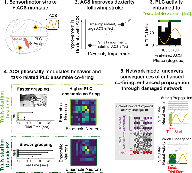
Graphical Abstract

Introduction

The time-varying activation of neural ensembles is an essential driver of behavior (Buzsáki, 2010; Harris, 2005; Hebb, 1949), yet it remains unknown how to precisely modulate ensembles using electrical stimulation. This knowledge gap prevents development of technologies that directly target the neural patterns underlying complex behaviors. For example, stimulation methods to improve motor function after stroke initially showed promise (Fregni et al., 2006; Plautz et al., 2003), but translational efforts were hampered by inconsistent results; two recent clinical trials failed to detect a benefit of stimulation (Harvey et al., 2018; Levy et al., 2016). These studies typically delivered stimulation continuously, without knowledge of the current state of neural patterns and behavior. In contrast, understanding how stimulation directly alters neural patterns and behavior has the potential to improve efficacy (Ganguly et al., 2013; Liu et al., 2018; Ramanathan et al., 2018). The neural patterns that produce behavior are driven by an interplay between “internal dynamics” and external environmental cues (Harris, 2005; Shenoy et al., 2013). Internal dynamics refers to the property that neural activity at a given time point can reliably predict future activity without apparent influence from external sources (Churchland et al., 2012; Harris et al., 2003; Luczak et al., 2007; Pastalkova et al., 2008). Internal dynamics are likely the result of network connectivity that produces time-varying ensemble activations without need for external drive (Diesmann et al., 1999; Lemke et al., 2019; Luczak et al., 2009; Rajan et al., 2016; Sussillo et al., 2015).

How then can electrical stimulation, which is not sensitive to internal dynamics, be used therapeutically to assist neural processing and boost motor function after stroke? We focus on epidural electrical stimulation approaches since they are relatively less invasive and are promising for translation (Levy et al., 2016; Liu et al., 2018; Ozen et al., 2010; Ramanathan et al., 2018). Studies in vitro and in anesthetized animals have found that externally applied fields, static or oscillatory, can grossly boost firing rates (Bergmann et al., 2009; Bindman et al., 1962; Feurra et al., 2011) and bias spike timing (Ali et al., 2013; Fröhlich and McCormick, 2010; Ozen et al., 2010). More recent studies confirmed these results in awake animals (Johnson et al., 2020; Krause et al., 2019). However, in the few studies where spiking activity was monitored during stimulation in behaving animals, expected neural changes predicted from in vitro and in vivo studies were not found (Berényi et al., 2012; Kar et al., 2017; Krause et al., 2017; Ozen et al., 2010). Thus, it remains unclear how stimulation can influence ensemble activity governed by internal dynamics.

The primary goal of this study was to assess how external stimulation directly interacts with impaired task-related neural patterns to improve neural processing and restore motor function following stroke. Past studies to improve motor outcomes following stroke have used continuously delivered electrical stimulation to induce long-term plasticity (Cooperrider et al., 2014; Guggenmos et al., 2013; Plautz et al., 2003), with mixed clinical outcomes (Hao et al., 2013; Harvey et al., 2018; Levy et al., 2016). In contrast, relatively little attention has been paid to how electrical stimulation immediately and directly influences task-specific neural patterns (Liu et al., 2018; Ramanathan et al., 2018). We thus monitored “perilesional” cortex (PLC) patterns during sham and stimulation while non-human primates recovering from either a motor or sensorimotor cortical stroke (Darling et al., 2016; Morecraft et al., 2015) performed a reach-to-grasp task. We found a significant improvement in dexterity with low-frequency alternating current stimulation (ACS). We also found that ACS increased co-firing in task-related PLC ensembles during dexterous behavior. Notably, these changes resembled increases in co-firing observed during recovery. To further explore how changes in co-firing may be linked to improved function, we developed a neural network model of the PLC. This model revealed that increases in co-firing driven by ACS allowed for more reliable activity propagation. Together, our results demonstrate how oscillatory stimulation can directly modulate impaired task-related neural patterns after stroke and improve function.

Results

Recovery of dexterity from an M1 stroke

Rhesus macaques were trained to perform a pellet-retrieval task (Fig. 1A). Animals retrieved pellets from wells of varying diameters. Trial time varied depending on well size (Fig. S1). Animals were trained until performance plateaued. Next, animals underwent stroke induction in which the right hemisphere primary motor cortex (M1) arm and hand area was targeted with surface vessel occlusion followed by subpial aspiration (Darling et al., 2009). Surgical images were used to illustrate lesions (Fig. S2). In a subset of animals, ex-vivo MRIs confirmed lesion location (Fig. 1B). In the same surgery, microwire electrode arrays were implanted in the PLC. Following a period of recovery, animals were behaviorally tested.

Figure 1: Improved behavior and consistency of PLC sequential firing with recovery.

(A) Pellet retrieval task paradigm.

(B) Top Lesion and electrode array location Bottom left, intact M1 (Rohlfing et al., 2012) accessed via The Scalable Brain Atlas (Bakker et al., 2015). Bottom right, ex-vivo MRI from Monkey Bl illustrating lesion. See also Fig. S2

(C) Example index finger trajectories from Monkey H during an intermediate session (top) and following full recovery (bottom). See also Fig. S1.

(D) Behavioral improvements in 3 animals performing the pellet task. Baseline normalized R2G (LME with animal as random effect, t₅₄₄ = −6.161, p = 7.22×10⁻¹⁰), normalized reach duration (t₅₄₄ = −4.457, p = 8.31×10⁻⁶), and normalized grasp duration (t₅₄₄ = −5.902, p = 3.58×10⁻⁹) over recovery. Lines show LME fits with animal-specific intercepts.

(E) Fast, successful trial-averaged templates (left column) and single trials (right column) aligned to reach start (RS) during “intermediate” recovery (top row) and full recovery (bottom row).

(F) Template match over recovery (LME with animal as random effect, t₃₃₄ = 6.193, p = 5.92×10⁻¹⁰). Bars indicate mean (sem) over trials. Gray lines indicate average trend per animal.

(G) Normalized R2G time is significantly negatively correlated with template match (LME, animal as a random effect on slope and intercept: t₅₈ = −2.409, p = 0.016). Individual points are means (sem) of trials binned into twenty equal sample size bins based on normalized R2G times. Lines indicate animal-specific slope and intercept fit by LME model. See also Fig. S3

(H) Example of non-multiphasic and multiphasic trial-averaged unit activity aligned to reach start (RS), quantified by assessing if the autocorrelation (middle column) exhibited a significant peak between 0.1–0.5 seconds. (Right) Timing of peak (non-multi phasic) or peaks (multiphasic) of trial-averaged activity for task-modulated units pooled over three animals.

As expected, behavior improved over time. Example index finger trajectories from impaired and recovered trials are plotted in Fig. 1C. Early in recovery, animals were slow at performing the task for the more difficult, smaller wells. When animals fully recovered, they could quickly retrieve the pellet from all wells. Recovery was quantified by measuring “reach duration” (time to transport hand from “start” to the well), “grasp duration” (from end of reach to having stable control of the pellet), and “reach-to-grasp time” (sum of reach and grasp, hereafter R2G). These metrics were normalized by their respective average pre-stroke times on the same well size. For successful trials, there were significant improvements in normalized R2G time (LME, animal as random effect t₅₄₄ = −6.161, p = 7.22×10⁻¹⁰), normalized reach duration (t₅₄₄=−4.457, p = 8.31×10⁻⁶) and normalized grasp duration (t₅₄₄ = −5.902, p = 3.58×10⁻⁹).

Consistent sequential neural patterns emerge with recovery

We next characterized changes in task-related neural activity over recovery. Single units in PLC were binned, temporally smoothed, and z-scored. Single trial PLC patterns were then compared to a template of behaviorally successful PLC patterns per session. Session-specific templates were computed since the exact single-unit population recorded varied over recovery. Behavior in single trials early in recovery was slower on average, but a subset of trials were executed quickly and successfully. Averaging PLC activity over these fast, rewarded trials on each day of recovery yielded a template that estimated the PLC pattern for successful behavior (Fig. 1E, left column).

We observed that similarity of single trials to the trial-averaged template tracked improvements (Fig. 1F–G). Similarity was estimated by computing the correlation coefficient (“template match”) between single trials and the template. Differences in numbers of units and numbers of fast, rewarded trials over recovery were accounted for by averaging template match estimates for each trial over many templates subselected to match unit and trial numbers. Example trial templates from an impaired (top) and recovered (bottom) sessions are shown in Fig. 1E left; single trials from the same session are shown in Fig. 1E right. There was an increase in template match with recovery. To quantify this, the first two sessions post-stroke with more than 5 rewarded trials were designated as “early”, and the sessions in which R2G trial times were not significantly different than the pre-stroke behavior were designated as “recovered”. All sessions in between “early” and “recovered” were designated as “intermediate”. Since different animals had different rates of recovery, “early”, “intermediate”, and “recovered” stages were determined for each animal.

Single trial template matching significantly increased over recovery (Fig. 1F, LME with animal as random effect t₃₃₄ = 6.193, p = 5.92×10⁻¹⁰). To assess if template match improvements correlated with behavioral improvement, linear regression was conducted between normalized R2G time and template match. For visualization, trials were grouped into twenty equally sized bins based on normalized R2G time, and averaged into a single point. Mean of binned template matching was significantly negatively correlated with mean of binned normalized R2G time (Fig. 1G, LME with animal as a random effect on slope and intercept: t₅₈ = −2.409, p = 0.016). Thus, with recovery, PLC activity became more similar to a template for successful behavior. We also tested whether the low frequency band of the local field potential (LFP) exhibited changes in consistency (Bönstrup et al., 2019; Lemke et al., 2019; Ramanathan et al., 2018). Similar to these studies, we found an increase in low frequency LFP phase consistency with recovery (Fig. S3 H–J).

We further characterized the underlying spatiotemporal structure of spiking in the recovered state and found it resembled a sequence of phasically active units. Sequential patterns are high dimensional and exhibit consistent temporal structure; we observed increases in dimensionality and predictability of single trial temporal dynamics with recovery (Fig. S3 A–G). To further elucidate the structure of PLC patterns, trial-averaged activity was analyzed (Fig 1H) to assess what fraction of units were sparsely active (monophasic) versus multiphasic (Churchland and Shenoy, 2007; Lemke et al., 2019). Aggregated over all three animals and recovered sessions, 22.0% of units were classified as multiphasic. Units were further classified as task-modulated, and of these, only 8.9% were multiphasic. Fig. 1H right illustrates the timing of the peaks of all task-modulated mono and multiphasic units. Thus, task-modulated units in the recovered state were primarily monophasic and population activity was high dimensional and temporally predictable, consistent with a sequential structure.

Epidural ACS enhances dexterity

When animals were in the impaired “intermediate” stage, 3Hz ACS was delivered on a subset of sessions (Fig 2A–B, yellow arrows). In this stage, reaching had largely recovered, but grasping deficits remained. ACS was compared to sham sessions that were performed on the same or an adjacent day. Session order was randomized. Low frequency ACS was chosen as a compromise between DCS, which was previously shown to improve R2G in rat stroke models (Ramanathan et al., 2018), and a charge-balanced paradigm which is more clinically translatable for an invasive device. ACS was turned on during behavioral sessions (open loop, lasting 10–15 minutes) without intentional alignment to trial structure (Fig 2A). ACS was off outside of behavioral sessions. ACS was delivered between pairs of stainless steel or titanium cranial screws positioned posterior to the lesion in the right hemisphere and anterior to the lesion in the left hemisphere, matching the efficacious orientation in Ramanathan et al., 2018 (Fig. 2A, Table S1 for animal-specific doses).

Figure 2: Open-loop epidural ACS improves dexterity.

(A) Open loop epidural ACS stimulation protocol

(B) Recovery of normalized R2G time for two animals performing pellet retrieval task. Yellow arrows indicate stimulation sessions.

(C) Significant improvements in pellet retrieval R2G time with ACS (LME with animal, ACS day, and well size as random effects: t₃₂₆ = −3.08, p = 0.0021), no change in reach duration (t₃₂₆ = 0.618, p = 0.537), and significant reduction in grasp duration (t₃₂₆ = −3.148, p = 0.00165). Bars are means (sem) over trials and each line is the mean for an animal, session, and well-size (Monkey H (Bl): black (gray)).

(D) For pellet retrieval task, significant correlation between sham grasp duration and effect of ACS (ACS minus sham grasp duration), (LME with animal as random effect: t₁₆ = −3.456, p = 0.000547). Each data point is the mean grasp duration of all trials for an animal, paired sham/ACS session, and well-size. Squares (circles) indicate data from Monkey H (Bl).

(E) Schematic of pinch-and-lift task and “gripper” objects that change task difficulty.

(F) Recovery of R2G time for two animals performing pinch-and-lift task. Left, Monkey Sb using flat, wide grippers. Center, Monkey Sb using narrow sloped grippers. Right, Monkey Sd using flat, wide grippers.

(G) Significant improvements in R2G time with ACS (LME, animal, ACS day, and gripper identity as random effects: t₉₀₄ = −3.143, p = 0.00167), no change in reach duration (t₈₈₆ = −0.401 p = 0.689), and significant reduction in grasp duration (t₈₈₆ = −3.104, p = 0.00191). Bars are mean (sem) over all trials and each black (gray) line is mean for each animal, day and grippers for Monkey Sd (Sb).

(H) For pinch-and-lift task, significant correlation between sham grasp duration and effect of ACS (ACS minus sham grasp duration), (LME with animal as random effect: t₁₁ = −2.708, p = 0.00676). Each point is the mean grasp duration for an animal, sham/ACS session pair, and gripper identity. Circles (squares, triangles) indicate data from Monkey Sb (Sb, Sd) for flat/wide (narrow/sloped, all) grippers.

See also Fig. S4

Epidural ACS improved dexterity in the pellet-retrieval task in two animals (third animal shown in Fig. 1 recovered too quickly, Table S1). ACS significantly reduced total R2G time (LME with animal, ACS day, and well size as random effects: t₃₂₆ = −3.08, p = 0.0021), driven by a significant reduction in grasp duration (t₃₂₆ = −3.148, p = 0.00165), and no significant change in reach duration (t₃₂₆ = 0.618, p = 0.537) (Fig. 2C). Video S1 shows a representative session with and without ACS.

In two additional animals, ACS improved dexterity in a separate R2G task, the “Pinch-and-Lift” task (Fig. 2E, F) (Brochier et al., 1999; Glees and Cole, 1950). One of these two animals received a motor cortical stroke (as previously described), while the second animal (Monkey Sd) received a sensorimotor stroke that included both M1 and primary somatosensory cortex (S1) (Darling et al., 2016). The task required use of the thumb and index fingers to lift an object from a slot (Fig. 2E). In contrast to the pellet retrieval task this task could only be accomplished using a pincer grip. Thus behavioral improvements could not simply be due to compensation with another grasp type (Ganguly et al., 2013; Krakauer, 2006). ACS significantly reduced R2G time (LME with animal, ACS day, and gripper identity as random effects: t₉₀₄ = −3.143, p = 0.00167), which was also driven by a significant reduction in grasp duration (t₈₈₆ = −3.104, p = 0.00191), and no significant change in reach duration (t₈₈₆ = −0.401 p = 0.689) (Fig. 2G). Video S2 shows a representative session with and without ACS.

For both sets of animals, we found that the greater the impairment, the greater the efficacy of ACS. Grasp duration impairment (grasp duration during sham sessions, x-axis), was significantly correlated with how strongly ACS improved grasp duration (ACS minus sham grasp duration, y-axis, Fig. 2D, pellet retrieval task, LME with animal as random effect: t₁₆ = −3.456, p = 0.000547, Fig. 2H, pinch-and-lift task : t₁₁ = −2.708, p = 0.00676). While this correlation may arise from a floor effect since the amount that grasp durations can reduce is limited, it is promising for clinical translation that large impairments benefit from ACS.

Finally, to investigate whether there were any ‘carryover’ effects once ACS was turned off, a subset of sessions where pre-ACS and post-ACS sham blocks were completed within the same day were analyzed, revealing no significant carryover effect of ACS (Fig. S4).

ACS entrains neural activity at a preferred phase

Next, we quantified how ACS influenced PLC units. Fig. 3B shows mean voltages, negative voltage gradient directions, and voltage gradient magnitudes for an example session from Monkey Sd. Negative voltage gradient directions (center) indicate estimates of current flow direction (other animals’ voltage gradient directions were comparable). The distribution of the electric field (voltage gradient magnitude) recorded in PLC during application of ACS (n=3, see Table S1) showed that mean field values ranged from ~2–4 mV/mm (Fig. 3C) and was consistently higher for animals who received higher amplitude ACS (Table S1). These field strengths are in the range previously shown to be efficacious for biasing neural activity (Liu et al., 2018). Using spiking data from the full 10–15 min session recordings, we estimated entrainment to ACS. Only two animals had sufficient unit recording quality to perform this analysis (Fig. 3D, see Fig S5 for example units and a discussion of recording challenges). Overall, 180 of the 316 units recorded from two animals (3 sessions/animal) were significantly entrained (57%). If units were restricted to putative single units, only 8 of 35 units were significantly entrained (23%).

Figure 3: ACS drives phases of neural excitability.

(A) PLC electrode array and ACS stimulation screws.

(B) Mean voltages (left), negative voltage gradient directions (middle), voltage gradient magnitudes (right) recorded on the PLC array when ACS waveform at peak (top row), intermediate point (middle row), and trough (bottom row) from an example session from Monkey Sd.

(C) Distribution of voltage gradients over channels and sessions for the peak (left), intermediate point (middle), and trough (right) of the ACS waveform. Arrows on x-axis indicate subject means.

(D) Example units recorded from Monkey H during ACS. Left (chan 48) is significantly entrained Right (chan 61) is not significantly entrained but shows slight phase preference. Example waveforms (gray), average waveforms (black), and ISIs (black histograms). See also Fig. S5.

(E) Distribution of preferred phases over all units (gray bars) and significantly entrained units (black bars) recorded during ACS for Monkey H (left) and Monkey Bl (right). Distributions are significantly non-uniform (Rayleigh test, Monkey H: all units, N = 163, z = 11.38, p = 9.68e-6, only significantly entrained units, N = 72, z = 12.70, p = 1.82e-6, Monkey Bl: all units; N = 153, z = 6.64, p = 0.00124, significantly entrained units, N = 108, z = 13.33, p = 1.11e-6). The designated “excitable zone” (light green bar) is illustrated above distributions.

We also observed a clear ACS phase preference across the population of all PLC units in each animal (Fig. 3E, gray bars) that was consistent even if only significantly entrained units were considered (Fig. 3E black bars). Distributions were significantly non-uniform (Rayleigh test, Monkey H: all units, N = 163, z = 11.38, p = 9.68e-6, sig. entrained units, N = 72, z = 12.70, p = 1.82e-6, Monkey Bl: all units; N = 153, z = 6.64, p = 0.00124, sig. entrained units, N = 108, z = 13.33, p = 1.11e-6). There was no significant difference between the distribution of all units and of significantly entrained units (Kuiper test, circular analog of KS test: Monkey H, test statistic = 2026., p = 1.0, Monkey Bl: test statistic = 2106., p = 1.0). Interestingly, units from Monkey H preferred the peak whereas units from Monkey Bl preferred the trough. The magnitude of the voltage gradient at the peak and trough were comparable but with opposite current flow direction (Fig. 3B–C). Geometric orientation of units to the electric field (Radman et al., 2009), current amplitude (Batsikadze et al., 2013), and the directional sensitivity of the network (Bikson et al., 2004) may all have influenced the preferred current direction. We next defined an animal-specific range of phases (circular mean +/− 1.5*95% circular confidence interval) that captured most units’ preferred phase. We called this window of animal-specific ACS preferred phases the neural “excitable zone” (EZ, light green bar, Fig. 3E).

Dexterity improves when trials are aligned to EZ

If the EZ, defined from PLC units’ preferred phase, was important for function we predicted differences in motor behavior based on EZ alignment. We fit a circular histogram to the distribution of preferred phases (Fig. 4A, left) and binned R2G time for a representative session from Monkey Bl by ACS phase at reach start (Fig. 4A right). We observed a correspondence between preferred phase and faster behavior for trials starting at preferred phases.

Figure 4: Behavior starting in the excitable zone is faster.

(A) Left: Circular histogram fit to distribution of preferred phases. Right: Example session from Monkey Bl, average (sem) R2G times binned by ACS phase at reach start superimposed with circular histogram fit of phase.

(B) Visualization of phase-dependency of grasp duration (purple, note inversion so faster R2G times higher on y-axis) and circular histogram fit to phase preferences (green, same as A).

(C) Mean outside EZ trials are significantly slower for R2G time (LME with animal, session, and well-size as random effects: t₁₀₁ = −2.15, p = 0.0315), not significantly different for reach duration (t₁₀₁ = 0.6465, p = 0.518), and significantly slower for grasp duration (t₁₀₁ = −2.086, p = 0.037). Bars indicate mean (sem) over trials. Black (Monkey H) and gray (Monkey Bl) dashed lines indicate average session trends. Solid lines indicate average trends pooled over sessions.

For visualization, we smoothed ACS phase at reach start versus R2G time (Fig. 4B, purple) using a non-parametric moving average. The curves were inverted with faster R2G times higher on the y-axis. To quantify ACS-phase effect on behavior, all trials were grouped as either “inside EZ” or “outside EZ” based on the phase of reach start. Trials were significantly faster inside EZ than outside EZ (Fig. 4C: LME with animal, session, and well-size as random effects, t₁₀₁ = −2.15, p = 0.0315) and grasp duration (t₁₀₁ = −2.086, p = 0.037) with no significant difference for reach duration (t₁₀₁ = 0.6465, p = 0.518). Thus, the EZ reflected periods of network-wide change that significantly influenced behavior.

ACS drives phase-dependent increases in ensemble co-firing

We hypothesized that ACS phase may also influence task-related activity. Specifically, units that fired together in the task-related sequence may exhibit stronger co-firing due to the common influence from ACS. We split activity into “ensembles” consisting of distinct subsets of units that significantly modulated above baseline during i) reaching but not grasping (“reach”), ii) reaching and grasping (“reach-grasp”), or iii) grasping but not reaching (“grasp”) (Fig. S6A). The reach and reach-grasp ensembles were analyzed from −1.0–0.25s and −0.25–0.25s aligned to reach start respectively. The grasp ensemble was analyzed from −0.25–0.45s (Monkey H) or −0.25–0.85s (Monkey Bl), reflecting animal-specific average grasp duration.

We first analyzed modulation of trial-averaged unit activity. Fig. 5A illustrates raster plots and normalized mean traces for example units from the grasp ensemble. Over the full population there were no significant changes in unit modulation (Fig. 5B, LME with animal and session as random effects: reach ensemble: t₂₃₀ = 1.10, p = 0.27, reach-grasp ensemble: t₇₆=−0.429, p=0.668, grasp ensemble: t₅₀ = 0.0399, p=0.968). There was also no significant difference for ACS trials with reach start outside EZ vs. inside EZ (LME with animal and session as random effects: reach ensemble: t₂₃₀ = 1.88, p = 0.059, reach-grasp ensemble: t₇₆ = 0.944, p=0.345, grasp ensemble: t₅₀ = 1.140, p=0.254). We next analyzed pairwise correlations between pairs of units within an ensemble, and found no changes with ACS or inside vs. outside EZ trials (Fig. S6B–D). Thus, the effects of stimulation were not detectable at the level of single units or pairwise interactions. We did, however, observe that there were substantial changes in the off-diagonal values of the pairwise correlation matrices across conditions (Fig. S6B). Thus, ACS may modify a subset of pairwise interactions that is detectable at the level of ensemble correlations.

Figure 5: Phase-dependent increases in task ensemble co-firing with ACS.

(A) Top: Example grasp start (GS) aligned rasters from grasp ensemble units in Monkey H on day 23 (sham) and 24 (ACS). Bottom: Normalized trial-averaged activity for sham and ACS

(B) No significant differences in trial-averaged unit modulation for sham vs. ACS (LME, animal and session as random effects: reach ensemble: t₂₃₀ = 1.10, p = 0.27, reach-grasp ensemble: t₇₆=−0.429, p=0.668, grasp ensemble: t₅₀ = 0.0399, p=0.968). No significant differences in trial-averaged unit modulation for ACS trials with reach start outside EZ vs. inside EZ (reach ensemble: t₂₃₀ = 1.88, p = 0.059, reach-grasp ensemble: t₇₆ = 0.944, p=0.345, grasp ensemble: t₅₀ = 1.140, p=0.254). Bars indicate mean (sem) across all units. Black (gray) lines correspond to mean trends for each session pair for Monkey H (Bl).

(C) 1D-shared over total (1D-SOT) metric to assess co-firing. One-dimensional Factor Analysis model fit to ensemble data (as in bottom left equations), and 1D-SOT computed using model parameters. 2-neuron examples of high, medium, and low 1D-SOT (right).

(D) Reach and reach-grasp ensemble 1D-SOT is not significantly different for sham vs. ACS (LME, animal and session as random effects: reach:, t₁₀=0.524, p=0.600, reach-grasp: t₁₀ = −0.1945, p=0.846), but grasp ensemble 1D-SOT is significantly higher for ACS vs. sham (t₈ = 2.112, p = 0.0347). Bars indicate means (sem) over all animals and sessions. Black (Monkey H) and gray (Monkey Bl) lines correspond to 1D-SOT values for each session pair.

(E) Covariance matrices for grasp ensemble units for Monkey H days 23 (sham) and 24 (ACS).

(F) 1D-SOT is not significantly different for ACS outside EZ vs. inside EZ trials in reach ensemble (LME, animal and session as random effects: t₁₀ = 0.879, p = 0.379), but is significantly higher for trials with reach start inside EZ vs. outside EZ for the reach-grasp (t₁₀ = 3.359, p = 0.000782) and grasp ensembles (t₈ = 3.7076, p = 0.00021). Bars indicate means (sem) over animals and sessions. Black (Monkey H) and gray (Monkey Bl) lines correspond to 1D-SOT values for each condition pair.

(G) Covariance matrices for grasp ensemble units from Monkey H days 24 (ACS) for outside EZ and inside EZ trials.

See also Fig. S6

We quantified ensemble co-firing using a metric we termed “one dimensional shared over total variance” (1D-SOT, Fig. 5C), a modified version of the SOT metric (Athalye et al., 2017, 2018). Specifically, the 1D-SOT was derived by fitting a Factor Analysis (FA) model with a single shared dimension to ensemble activity. FA models population variance as a sum of low-dimensional sources of shared variance (co-firing), and high-dimensional sources of variance specific to each unit. FA was used instead of other dimensionality reduction methods to specifically model co-firing. A single shared dimension was used since the model was fit on ensembles, thereby already restricting to units that positively modulate in the analyzed time windows. Thus, ensemble shared variance was expected to be one-dimensional. Further, we aimed to assess whether ACS would affect the dominant shared variance dimension for each ensemble, making 1D-SOT comparisons appropriate. A high 1D-SOT value indicates high ensemble co-firing whereas a low 1D-SOT value indicates that ensemble units largely fire independently (Fig. 5C).

We compared the sham and ACS conditions and found that 1D-SOT was significantly higher in the grasp ensemble with ACS (Fig. 5D, LME with animal and session as random effects, t₈ = 2.112, p = 0.0347) and not significantly different for the reach (t₁₀=0.524, p=0.600) or reach-grasp ensemble (t₁₀= −0.1945, p=0.846). Increased off-diagonal components in grasp ensemble covariance matrices illustrate increased 1D-SOT (Fig. 5E). We then found that inside EZ 1D-SOT was significantly higher than outside EZ 1D-SOT for the reach-grasp (LME with animal and session as random effects: t₁₀ = 3.359, p = 0.000782) and grasp (t₈ = 3.7076, p = 0.00021) ensembles but not different for the reach ensemble (t₁₀ = 0.879, p = 0.379). The higher inside EZ versus outside EZ off diagonal components illustrate the higher 1D-SOT (Fig. 5G). Template match (Fig. 1), dimensionality, and temporal predictability (Fig. S3) were also analyzed, and ACS did not significantly affect these metrics (Fig S6). Thus, changes with ACS were not detectable in modulation of individual units (Fig. 5B) or pairwise interactions (Fig S6 B–D) but were clear at the ensemble correlation level (Fig. 5D–G).

Finally, given the increases in grasp-ensemble 1D-SOT with ACS, we wondered whether 1D-SOT also increased over the course of behavioral recovery. However, changes in neural activity from early to recovered sessions exhibited increases in dimensionality (Fig. S3C). Since higher dimensional signals directly reduce the amount of shared variance that can be absorbed by a single dimension, this change prevented a comparison of 1D-SOT from early to recovered sessions. Further, the same stably recorded units observed in early sessions were not always observed in later sessions, preventing a comparison of early session units to a subselection of the same units in late sessions. We thus sought to compare intermediate days to fully recovered days since the neural population did not exhibit significant changes in dimensionality (LME with animal as random effect t₁₀ = −0.1747, p = 0.8613). There was a significant increase in 1D-SOT computed from the full population of units within the R2G time period (−0.25 to 0.25 seconds aligned to grasp start, LME with animal as random effect, t₈ = 2.29, p = 0.0219). Thus, increases in 1D-SOT could account for the immediate effects of stimulation and the improvements in behavior over late stage recovery.

Overall, the preferred phases of ACS corresponded to increased neural excitability (EZ) which increased grasp ensemble co-firing especially when behavior started within the EZ. This increased co-firing may reflect neural patterns that resemble a more “recovered state”, and may account for improved dexterity.

A neural network model of stroke, ACS, and sequence propagation

Our results suggest that changes in task-related ensemble firing is linked to improvements in dexterity. We next established a model of an impaired PLC to explore the relationship between ACS, co-firing, and propagation of neural sequences.

To model an impaired PLC, we modified a synfire network that was designed to produce sequential activity (Diesmann et al., 1999; Gewaltig et al., 2001), emulating the R2G-related PLC patterns observed in the recovered state and in intact animals from other studies (Lecas et al., 1986; Rouse and Schieber, 2016a, 2016b; Veuthey et al., 2020). To model impairment, parts of the network had reduced internal connectivity (Fig. 6A, Table S2). Premotor PLC rewiring is critical for recovery, and reduced internal network connectivity reflected incomplete rewiring. Specifically, following M1 lesions, hand movement representation within premotor (PLC) motor maps have been shown to expand in area (Frost et al., 2003; Liu and Rouiller, 1999; Nudo, 1997). Changes in premotor maps are correlated with behavioral recovery (Ramanathan et al., 2006). Premotor PLC also has anatomical projections to subcortical targets that can drive both proximal and distal movements enabling its role in recovery (Darling et al., 2018; Dum and Strick, 1991). Furthermore, we interpret the sequential neural activity that emerged with recovery (Fig. 1, Fig. S3) to reflect a PLC network that developed internal connections to produce neural patterns for successful R2G actions. We focus here on modeling changes within premotor PLC as they correlate with recovery and ACS-related improvements.

Figure 6: A neural network model of PLC links ACS, ensemble co-firing, and neural sequence propagation.

(A) Neural network with input (red), fully connected (gray) and impaired subnetwork (purple). See also Fig. S7.

(B) Statistics of input spikes (σ, N) influence sequence propagation: left: (8ms, 145 spikes), center: (8ms, 300 spikes), and right: (0ms, 145 spikes).

(C) Impaired R2G input parameters. Left, 25ms, 350 spikes, Right 2ms, 60 spikes.

(D) Sequence propagation for input parameters (σ, N) on x, y axes. Pixels inside white boxed regions correspond to impaired R2G input parameters.

(E) Distribution of preferred phases of simulated neurons during ACS (gray bars). EZ is centered on circular mean of distribution (+/− π/4).

(F) 1D-SOT significantly changes for sham vs. ACS and Outside vs. Inside EZ for all ensembles. (LME, input parameter as random effect: Top, sham vs. ACS: pool 1: t₃₆ = −10.03, p < 1.08e-23, pool 43:, t₃₆ = 9.38, p < 6.45 e-21, pool 53: t₃₆ = 8.61, p < 7.05e-18. Bottom outside EZ vs. inside EZ, pool 1: t₃₆= 24.77, p < 1.87e-135, pool 43: t₃₆= 13.23, p < 5.7e-40, pool 53: t₃₆= 11.51, p < 1.18e-30)

(G) A short propagation sequence (left). Input aligned to EZ can improve (center), or worsen propagation (right).

(H) Change in sequence propagation (ACS – sham) over all impaired R2G inputs (x-axis) for alignment of input to ACS phase (y-axis).

(I) Correlation between change in 1D-SOT in grasp ensemble vs. change in propagation (linear correlation, r = 0.89, p < 3.77e-59, N = 171). Each point is average over many simulations for each impaired R2G input parameter-by-ACS-phase combination.

Specifically, the PLC model was composed of a fully connected “reach” subnetwork (43 pools, 100% inter-pool connectivity) connected to an incompletely formed “grasp” subnetwork (43 pools, 85% inter-pool connectivity, Fig. 6A, Fig. S7, Table S2) with pools comprised of 100 integrate-and-fire neurons. The model had impaired neural sequence production (Fig S7E) and activity patterns that replicated our experimentally observed reductions in template matching, dimensionality, and temporal predictability found early after stroke (Fig 1., Fig. S3 and S7F–G). Importantly, the timing between the start of the “reach” subnetwork and the start of the “grasp” subnetwork was ~258ms, matched to experimental data (Monkey H: 260 ms, Monkey Bl: 253 ms). R2G neural patterns in the network were initiated by an “input” spike train that consisted of N spikes drawn from a Gaussian distribution with mean (μ) and standard deviation (σ) (Fig. 6C). Input properties influenced activity propagation. Fig 6B left illustrates input parameters that did not fully propagate. An increase in N (center) or a decrease in σ (right) allowed full propagation.

We considered activity propagation as a proxy for quality of R2G behavior where poorly propagating activity corresponded to poor movements. We selected input parameters where activity was successfully initiated but exhibited incomplete propagation to model intact reaching and impaired grasping, as when we testing ACS. “Sequence propagation” was defined as the correlation between simulated activity and an ideal, fully propagated template sequence (Fig. 6D). White lines illustrate input parameters (σ, N) where sequence propagation was incomplete but initiated.

We applied ACS to the model and found entrained network activity and phase-dependent improvements in propagation. ACS was modeled as a sinusoidal current injected directly into each neuron. Units exhibited entrainment to the ongoing sine wave (Fig. 6E). As in the experimental data, the EZ was computed from the distribution of preferred phase of all units (Fig. 6E). When simulating activity with ongoing ACS, if the mean of the input spike train (μ) was inside the EZ, propagation improved (Fig. 6G center) compared to activity simulations without ACS (Fig. 6G left). When the same input spike train was outside the EZ, propagation worsened (Fig. 6G, right). Generally, when input spike trains were centered on the EZ, sequence propagation improved. Changes in propagation (Fig. 6H) depended on input parameters (x-axis) and alignment to ACS phase (y-axis). Input spike trains starting inside the EZ improved propagation (red) compared to the no-ACS (sham) condition.

As in the experimental data, simulated patterns were analyzed for changes in 1D-SOT. The 1^st, 43^rd, and 53^rd pools were analyzed to assess “reach”, “reach-grasp”, and “grasp” ensemble 1D-SOT, as in Fig. 5 (pools marked with horizontal arrows to the right of Fig. 6G right). We found 1D-SOT significantly increased for sham vs. ACS and Outside vs. Inside EZ for all ensembles except sham vs. ACS for the reach ensemble (Fig. 6F LME with input parameter as random effect: Top, sham vs. ACS: pool 1: t₃₆ = −10.03, p < 1.08e-23, pool 43: t₃₆ = 9.38, p < 6.45 e-21, pool 53: t₃₆= 8.61, p < 7.05e-18. Bottom outside EZ vs. inside EZ, pool 1: t₃₆= 24.77, p < 1.87e-135, pool 43: t₃₆ = 13.23, p < 5.7e-40, pool 53: t₃₆ = 11.51, p < 1.18e-30). As in Fig. 5D–G, 1D-SOT effects are stronger for the inside vs. outside EZ comparisons compared to the sham vs. ACS comparisons. Effects are also strongest for the later activating reach-grasp and grasp ensembles compared to the reach ensemble.

We wondered whether there was a link between changes in 1D-SOT and changes in propagation. We found that changes in 1D-SOT observed in the “grasp” ensemble were strongly predictive of sequence propagation (Fig. 6I, linear regression, slope = 1.58, r = 0.89, p < 3.77e-59, N = 171). This result draws a putative link between the phase-dependent increases in 1D-SOT observed in the experimental data (Fig. 5) and the phase-dependent improvements in behavior observed (Fig. 4). Increased grasp co-firing may reflect neural patterns with improved propagation, and therefore improved behavior.

ACS waveform optimization

Can we design a charge-balanced stimulation waveform that improves propagation in a less phase-dependent manner? We tracked the “mean-effect” and “phase-effect” to compare different stimulation paradigms (Fig. 7A). Mean effect was mean improvement in sequence propagation computed over all input parameters and ACS phases. Phase effect reflected the phase dependence of improvements. Ideal stimulation would have low phase (x-axis) and high mean effects (y-axis, purple region, Fig. 7B).

Figure 7: Waveform optimization to enhance propagation.

(A) “Mean effect” and “Phase-effect” quantification. Left: Gray lines are change in propagation as function of input alignment to ACS phase for each impaired R2G input parameter, Right: Black line is average over all input parameters. “Mean effect” is average of black line and “phase effect” is std. of black line.

(B) Phase-effect vs. mean-effect space: ideal stimulation has a low phase-effect and high mean-effect (purple).

(C) Phase-effect vs. mean-effect for varying amplitudes (in nanoamps) of 3 Hz ACS. Circled point indicates amplitude used in Fig. 6.

(D) ACS amplitude affects sequence propagation when input is delivered inside EZ (left plots in each column) and outside EZ (right plots in each column). Sequences are red for visualization.

(E) Phase-effect vs. mean-effect for different ACS frequencies.</p/> F) Phase-effect vs. mean-effect for designed waveforms. Colors denote waveform shape (maroon = single negative half-cycle, orange = multiple negative half-cycles). Frequency labels denote the frequency of the negative half-cycle.

(G) Optimized waveform (+3Hz, single half-cycle −10Hz) improves sequence propagation (right) compared to 3Hz ACS (left) for same inputs.

(H) Comparison between 3Hz ACS (left) and optimized waveform (+3Hz, single phase −10Hz, right) sequence propagation length. Color indicates change in propagation length (units of # pools) compared to non-ACS for a given input parameter set (y-axis) at a given phase of the waveform (x-axis). Red and blue indicate lengthening and shortening in propagation respectively.

(I) Phase-effect vs. mean-effect in units of “change in pools propagated” instead of “change in sequence propagation metric” (as in Fig. 7B-C, E-F). For 3 Hz ACS (black), ACS extends propagation by a mean-effect (phase-effect) of 11.2 (15.5) pools. Optimized waveform (maroon) extends propagation by 18.9 (13.5) pools.

We first explored changing the amplitude of 3Hz ACS (Fig. 7C). While increased amplitude increased the mean effect, there was increased phase-effects up to 75nA, after which both effects reduced. Above 75nA, amplitude was so high it started to drive neural sequences at unintended times (Fig. 7D center) or completely entrain neurons, preventing sequence production (Fig. 7D right). While entrainment is viewed as beneficial, these results suggest that excess entrainment can subsume intrinsic dynamics.

We next explored changing ACS frequency (constant amplitude). Low frequencies (blue, Fig. 7E) were efficacious, but had large phase-effects. High frequencies were ineffective at improving sequence propagation, due to neuron membrane time constants preventing integration of high frequency inputs. Theoretically, higher frequencies could be efficacious, but would require much higher amplitudes.

Can a more efficacious, charge-balanced stimulation waveform be designed using the principle that low frequencies influence membrane voltages more than high frequencies? In order to keep the efficacious EZ of the 3 Hz waveform and reduce the detrimental phases (Fig. 6H), we created a new waveform by adjoining a positive half cycle of the 3 Hz waveform to one or many negative half-cycles of a higher frequency waveform (Fig. 7F, right). Overall, the waveform with the single negative half-cycle (maroon) improved most upon standard 3Hz ACS by reducing the phase effect and improving mean effect (Fig. 7F left). Examples in Fig. 7G illustrate that the reduced duration of the negative half-cycle of the designed waveforms may assist with sequence propagation.

We further quantified the efficacy of the optimized waveform (specifically, +3hz and −10 Hz waveform) by computing length of sequence propagation, or how many more pools the sequence travels before failure compared to no simulation. Over all input parameters assessed, the designed waveform propagated ~19 pools further than no stimulation (vs ~11 pools for 3Hz ACS). Averaged over all input parameters (y-axis of Fig. 7H), the optimized waveform improved sequence propagation for all 9/9 phases compared to only 5/9 phases for 3 Hz ACS. The designed waveform is thus closer to the “ideal” purple region (Fig. 7F, I). In contrast, changes in stimulation amplitude or frequency could only jointly increase or decrease the mean and phase effects together (Fig. 7C, E). While future work must validate these simulations in vivo, they reveal principles of how to design external modulation to optimize propagation.

Discussion

In summary, we demonstrate that epidural low-frequency ACS in primates recovering from stroke can significantly improve dexterity in two different R2G tasks. ACS improved dexterity in a phase-dependent manner. Moreover, task-related ensembles exhibited increases in co-firing for trials with reach starting inside EZ. A model of impaired PLC ties increases in co-firing to improved activity propagation. Overall, these findings demonstrate how externally applied ACS can interact with and enhance internal processing and restore dexterity after stroke.

Reemergence of sequential activity with recovery

Recovered task-related activity was largely comprised of a sequence of monophasic neural activations (Fig. 1). Previous work in motor areas has found evidence for sequential structure during well learned R2G tasks in intact animals (Lecas et al., 1986; Murphy et al., 1985; Riehle et al., 2013). Further, a neural network model designed to produce sequential activity exhibited increases in template matching, dimensionality, and temporal predictability with increasing internal connectivity (Fig. S7), as was observed in experimental data with recovery (Fig. 1, Fig. S3). Thus, stroke interrupted network function and PLC connectivity, with recovery reinstating reliable, high-dimensional, predictable activity patterns. As highlighted in Lebedev et al., 2019, a population where units are monophasically activated at consistent time lags will produce rotational dynamics making our findings of sequential patterns consistent with studies of rotational dynamics in premotor cortex and M1 (Churchland et al., 2012; Sussillo et al., 2015).

What might this sequential structure encode? Sequential activity during R2G tasks may reflect a sequential drive of proximal then distal muscles (Lecas et al., 1986; Rouse and Schieber, 2016a, 2016b). Alternatively motor cortical areas may not directly generate movement, instead sequentially coordinating downstream areas that drive movement (Buford and Davidson, 2004; Darling et al., 2018; Fetz et al., 2000; Lawrence and Kuypers, 1968a; Lemke et al., 2019; Lemon, 2008; Riddle et al., 2009; Zaaimi et al., 2012). Sequential patterns may also serve a role in maintaining timing between sub-movements (Hall et al., 2014), higher level task timing (Karmarkar and Buonomano, 2007; Remington et al., 2018), or tracking sensory feedback (Hatsopoulos and Suminski, 2011). How exactly sequential activity is related to movement control is unclear, but our results support that behavioral recovery following M1 damage occurs concomitantly with the re-emergence of reliable, temporally predictable, neural sequences in the PLC.

Neuromodulation entrains neural activity

Our study provides strong evidence that low-frequency ACS directly influences network activity and improves dexterity. We found that epidural ACS entrained ~60% of recorded units in awake-behaving animals, more than in previous studies (Johnson et al., 2020; Krause et al., 2019; Ozen et al., 2010). When we restricted to putative single-units, ~ 23% were entrained, comparable to these studies. Discrepancies across studies could be explained by differences in stimulation fields (~2–4 V/m here vs. ~1V/m in Ozen et al., 2010, < 0.5V/m in Krause et. al., 2019, 0.2–1.2V/m in Johnson et. al. 2020), frequency of stimulation, gyrated vs lissencephalic cortex, recording site, behavioral or anesthesia state, or unit properties.

We also found that for different animals, PLC units exhibited different phase preferences. However, after identifying each animals’ preferred phase of ACS, we found a clear link between preferred phase and behavior quality. Both preferences were at the maximal voltage gradient magnitudes, but differed in gradient direction. In vitro and in vivo work has shown that direction of current flow affects neural modulation (Bikson et al., 2004; Radman et al., 2009; Rawji et al., 2018). In gyrated brains, there is considerable variation in neuron orientation, complicating predictions of sensitivity to direction (Datta et al., 2009; Huang et al., 2017). Further complicating comparisons, stimulation amplitude can modify effects. For example, increasing the amplitude of cathodal tDCS from 1mA to 2mA makes the typically inhibitory effect excitatory (Batsikadze et al., 2013). It is possible that since amplitude and lesion location varied across animals, different current directions were efficacious for each animal.

Neuromodulation enhances propagation of sequences

ACS increased task-related PLC ensemble co-firing in a phase-dependent manner, mirroring phase-dependent dexterity improvements. To our knowledge, this is the first evidence of epidural stimulation driving changes in task-related ensemble spiking. To further explore how co-firing may improve behavior, we developed a model of the recovering PLC. In the model, we found that when ACS increased 1D-SOT (phase-dependent), sequence propagation improved. Since we considered propagation a proxy for R2G behavior, these findings link experimental findings of ACS-driven increases in co-firing to improved behavior. Further, in the brain, each “pool” likely has a downstream target (subcortical network or muscle). Thus, increased co-firing within the network may also assist with propagation to subcortical targets; boosting neural propagation may be a key therapeutic target for ACS.

While our model captured features from our experimental results and allowed us to design novel stimulation waveforms, it was a purely excitatory feedforward network without recurrent connections. Feedforward sequences can be embedded within randomly connected networks (Aviel et al., 2005; Trengove et al., 2013) or cortical networks (Kumar et al., 2008). Recurrently connected random networks can also produce sequential activity (Hardy and Buonomano, 2017; Rajan et al., 2016). Future work can assess how stimulation interacts with recurrently connected networks with both excitatory and inhibitory populations.

Direct neuromodulation

Our results suggest that open-loop low-frequency ACS may improve dexterity in stroke patients. The use of cranial screws to deliver epidural stimulation is relatively less invasive (Ramanathan et al., 2018) compared to deep brain stimulation or subdural stimulation. Moreover, cranial screw based stimulation avoids concerns regarding current shunting through the skin, muscle, skull, or neck in non-invasive approaches (Vöröslakos et al., 2018). Current paths taken due to current shunting may modulate peripheral nerves or off-target brain regions, confounding results. In this work, current shunting through the skull is possible. The most likely path was via the craniotomy defect, which was covered with non-conductive bone cement, thus making extracranial peripheral stimulation unlikely. Notably, while our measured electrical fields suggest the need for an invasive approach, it is possible that non-invasive methods may eventually allow reliable modulation of cortical structures (Grossman et al., 2017; Johnson et al., 2020). Lastly, our approach was effective for both motor cortical strokes and one larger sensorimotor stroke (Monkey Sd). Future work can assess whether this modulation approach will be efficacious for larger strokes.

While our approach was to assess the direct consequences of ACS on neural activity and behavior, it is unclear if sustained exposure can result in long-term plasticity. Our data suggests there were not short-term carryover effects of stimulation (Fig. S4), but longer stimulation sessions could result in carryover effects. ACS-driven increases in co-firing could improve dexterity and assist in PLC network recovery through Hebbian plasticity mechanisms (Plautz et al., 2003). Notably, our animals did fully recover over time; future studies can determine whether rehabilitation with ACS can accelerate this recovery.

Low-frequency oscillations, spiking, and epidural stimulation

Past work identified LFP low frequency oscillations (LFOs) as a marker of successful movement execution that also tracks recovery (Bönstrup et al., 2019; Hall et al., 2014; Lemke et al., 2019; Ramanathan et al., 2018). Here, we found that LFO phase consistency increased with recovery (Fig. S3H–J). Further, our recent work in a rodent stroke model highlighted that direct current stimulation could improve reaching and increase task-related LFO power (Ramanathan et al., 2018), perhaps consistent with our observations that ACS increased co-firing. These results suggest that increased LFO power may reflect co-firing that is boosted with stimulation to enhance behavior. Interestingly, stimulation was most efficacious when delivered at specific times with respect to behavior, congruent with our findings that ACS was efficacious when reach start aligned to the EZ. Thus, if our paradigm operated in “closed-loop”, it may be possible to reduce total current injected and align the EZ to movement onset. Together, our results suggest that epidural stimulation can be effective in both rodent and primate stroke models and that stimulation induced changes in task ensemble co-firing underlie improved dexterity.

STAR Methods

RESOURCE AVAILABILITY

Lead Contact

Further information and requests for resources should be directed to and will be fulfilled by the Lead Contact, Karunesh Ganguly (karunesh.ganguly@ucsf.edu).

Materials Availability

This study did not generate new unique reagents.

Data and Code Availability

The data and custom code that support the findings from this study are available from the Lead Contact upon reasonable request.

EXPERIMENTAL MODEL AND SUBJECT DETAILS

Macaques

Experiments were conducted in compliance with the NIH Guide for the Care and Use of Laboratory Animals and were approved by the University of California, Davis Institutional Animal Care and Use Committee. A total of five adult healthy rhesus macaques (macaca mulatta) were used in experiments. Animals were 5–6 years old and 12.0–15.0 kilograms. Four of five animals were pair-housed and one animal was singly housed. Animals were housed in rooms with lights that turned on at 6am and off at 6pm. Of the five animals, three animals exhibited sufficient quality neural recordings to monitor over the course of recovery and ACS was tested in four animals (one animal recovered too quickly). See Table S1 for details.

METHOD DETAILS

Animal care and surgery

Lesion

Following task training, animals underwent a stroke-induction and microelectrode array implantation surgery. Preoperatively, animals were sedated with ketamine hydrocholoride (10 mg/kg), administered atropine sulfate (0.05 mg/kg), prepared and intubated. They were then placed on a mechanical ventilator and maintained on isoflurane inhalation (1.2–1.5%). Animals were positioned in a stereotactic frame (David Kopf Instruments, Tujunga, CA) and administered mannitol (1.5 g/kg) intravenously prior to the craniotomy (note that two animals did not receive mannitol in an effort to improve microelectrode array insertion). A skin incision, bone flap, and dural flap were made over the lateral frontoparietal convexity of the hemisphere and the caudal region of the frontal lobe and rostral region of the parietal lobe was exposed unilaterally. After cortical exposure, the lesion was induced using surface vessel coagulation/occlusion followed by subpial aspiration (Darling et al., 2009). In three of the five animals (Monkey Bl, Monkey H, Monkey Ba,), the lesion target was the forelimb region of primary motor cortex (M1) using anatomical landmarks. Specifically, the lesion extended dorsally to a horizontal level including the precentral dimple (the lateral-most part of the of the M1 leg area) and ventrally to the central sulcus genu (the dorsal most part of the M1 face area). In one animal (Monkey Sb), the central sulcus was slightly expanded, and the rostral bank of precentral gyrus was targeted constituting a lesion in the forelimb region of the “new M1” (Dum and Strick, 2002). Finally, in one animal (Monkey Sd), the forelimb region of the surface of both precentral and postcentral gyri were included in the lesion, constituting a sensorimotor lesion. Following resection, a flap of the dura was sutured to cover the lesioned area, while leaving a small window anterior and posterior to the lesion for electrode implantation. Drawings of all 5 animals’ lesions are illustrated in Fig. S2 based on photographs taken during surgery.

Microwire implantation

An 8×8 tungsten microwire multielectrode array with 500um electrode spacing in both dimensions (Tucker-Davis Technology, Alachua, FL) was mounted to a micromanipulator, attached to the stereotax, and inserted 2mm into dorsal premotor cortex (PMd) using anatomical landmarks. Array ground and references were tied to titanium skull screws. Another multielectrode array was inserted in primary sensory cortex (S1, area 2) in all animals but was not analyzed in this study due to inconsistent recording quality.

Skull screws

For structural support 6–8 titanium screws (Gray Matter Research, Bozeman, MT) of length 3mm or 5mm were placed around the skull to serve as an anchor for a dental acrylic headcap that was used to secure the microwire electrodes in place and seal the craniotomy. Two or three titanium screws were also placed anterior on the left hemisphere from the craniotomy and lesion and served as one of the ACS stimulation contacts (top right screws in Fig. 2A). These screws were lowered such that they were in contact with the dura. The other stimulation contacts were 2–3 stainless steel screws (Depuy Synthes, Raynham, MA) of length 6mm or 8mm and were located just posterior to the craniotomy. Screws were confirmed to be in contact with the dura during surgery and post-mortem.

Following surgery, animals were administered analgesics and antibiotics, and were carefully monitored post-operatively for 7 days.

Reach-to-Grasp Behavior

Prior to surgery, macaques were trained to perform either the pellet retrieval task or the pinch-and-lift task (described below).

Pellet Retrieval Task

A custom-built, automated pellet retrieval task was used to assess forelimb function in three animals (Totten et al., 2018). Briefly, animals were seated in a primate chair outfitted with a door allowing them to interact with the pellet task. To initiate a trial, animals touched a “start screw” that was connected to a capacitive touch sensor. Holding the screw for the random hold time (uniformly distributed between 0.5 – 0.8 seconds) triggered the automated apparatus to release an edible pellet from an automated pellet dispenser (80209–190S,142 Lafayette Instrument, Lafayette, IN) into one of five “wells”. All five wells had depths of 5.9mm and diameters of either 13mm, 19mm, 25mm, 31mm, or 37mm, with the smaller wells making the pellet retrieval more challenging for animals. Animals had 5 seconds to retrieve the pellet from the well before the apparatus would rotate the well out of view. Animals performed 10–100 trials per day, depending on impairment.

Two cameras (CM3-U3–13Y3C-CS, Point Grey, Richmond, BC, Canada) were mounted to a stainless steel platform providing a side and top view of the animal performing the pellet retrieval task. Camera frames and touch sensor activity were synchronized using the electrophysiology recordings system (Tucker-Davis Technology, Alachua FL).

Offline, videos from individual trials were automatically parsed and manually reviewed to mark trial scores (success, attempt but failure, or no attempt) and behavioral time points. Time points that were manually marked include a) Reach start: time at which hand starts moving toward well from the capacitive start screw, b) Grasp start: time at which the hand arrives at the well, c) Grasp finish: time at which the pellet is in control and the hand starts to retract back towards the mouth. For trials scored as “no attempt”, no behavioral markers were noted. For trials scored as “attempt but failure”, only reach start and grasp start were noted. For trials marked as “success”, reach start, grasp start, and grasp finish were all marked. All analyses excluded trials scored as “no attempt”.

To produce kinematic trajectories in Fig 1C–D, Fig. S1, markerless tracking algorithm DeepLabCut was used to track parts of the hand that were consistently visible throughout the trial (Mathis et al., 2018)

Pinch-and-Lift Task

While the pellet retrieval task resembles many established methods to assess dexterity such as the Kluver board (Lawrence and Kuypers, 1968b; Nudo et al., 1996), we noticed that the unconstrained nature of the task allowed animals to succeed in the task using variable grasp strategies. In order to constrain the grasp portion of the task and specifically study the pinch grip, thought to be cortically dependent (Muir and Lemon, 1983), we developed a task we termed the ‘pinch-and-lift’ task (Brochier et al., 1999; Glees and Cole, 1950). Animals initiate a trial by touching a capacitive touch sensor. A sound cuing successfully contact served as the “go cue”. Animals then reached toward a 1.5cm × 4.0cm slot located 9 cm in front of the capacitive touch sensor. They reached their index and thumb into the slot to pinch and lift “grippers”. The grippers were custom-designed and 3D-printed. Grippers used in the pinch-and-lift task are illustrated in Fig. 2E. Grippers were mounted to a device that transmitted the pinch force to a piezo resistive force sensor (FlexiForce A201). Varying the height and width of the grippers varied the difficulty of the task and the amount of force that animals needed to complete the task. Grippers were broadly split into two categories. Grippers were either flat and wide and able to be pinched early after stroke or they were narrow and sloped and required more control and strength to pinch (Fig. 2E, F). The grippers were pinched together and then lifted 1.5cm to a height that allowed the grippers to interrupt an infrared beam (IR Break Beam Sensor, 3mm LED, Adafruit.com). Animals had to hold the device at the lifted height for 0.25 sec, following which they received a juice reward through a chair-mounted juice tube. Animals had 10 seconds to complete the pinch-and-lift successfully.

The same 2 cameras were used in this task as in the pellet retrieval task. An additional camera was positioned such that it had a lateral view the slot into in order to see index and thumb movements.

Trials were automatically scored as “rewarded” or “unrewarded” based on whether the object was lifted above the 1.5cm height threshold for the 0.25 second hold period. Reach start and grasp finish behavioral markers were determined automatically from the capacitive sensor offset after holding and IR sensor onset respectively. Grasp start was determined based on kinematics that were extracted with DeepLabCut (Mathis et al., 2018). Specifically, animal wrist position was tracked, and grasp start was marked when the wrist crossed the vertical plane at the front of the slot following release from capacitive touch sensor.

Note that in the pinch-and-lift task, automated hand tracking was used to identify the grasp start behavioral mark from video data (necessary for computation of reach duration and grasp duration but not reach-to-grasp time), and could not identify grasp start due to camera occlusion in 18 trials. However, reach start and grasp finish were identified from task sensors, so there are 18 more trials included in the statistics for reach-to-grasp-time than reach duration and grasp duration in Fig. 2G,H.

Behavioral Metrics

For the both tasks, reach duration was defined as the time between reach start and grasp start. Grasp duration was defined as the time between grasp start and grasp finish. Reach-to-grasp duration was defined as the time between reach start and grasp finish. Normalized reach time, grasp time, and reach-to-grasp time were computed in some cases in the pellet retrieval task (e.g. Fig. 1) in order to account for the differences in difficulty for different well-diameters. All metrics for were normalized by dividing by the average of the pre-stroke performance for that well (see Fig. S1 for pre-stroke averages). Finally, trials were label as “single grasp attempt” or “multi grasp attempt” depending on the number of grasp attempts needed to complete the trial.

In Fig. 1, all days where behavioral metrics were not significantly different from pre-stroke baseline (Student’s t-test comparing reach-to-grasp durations for wells performed that day) were considered in the “recovered” category. The “early” category was composed of the first two sessions where more than 5 rewarded trials were performed. “Intermediate” days were after “early” and before “recovered”. Note that rate of recovery varied from animal to animal including how soon they were able to participate in doing the tasks. Due to this, animals began participating in tasks at different days post stroke, and the animal-specific “early”, “intermediate”, and “recovered” phases fell at different days post stroke.

Electrophysiology

Single Unit Extraction

Raw neural signals were acquired at 24414.0625 Hz using Analog PZ5 Pre-amplifier, RZ2 Bioamplifier, and RS4 Data Streamer (Tucker-Davis Technology, Alachua, FL). Offline, signals were median subtracted (median computed on each bank of 16 channels in array) to reduce motion artifacts and external noise and then bandpass filtered between 300 Hz and 6000 Hz. Spikes were then extracted from signals using MountainSort (Chung et al., 2017). For the recovery datasets (Fig. 1, Fig S3), all waveforms with noise overlap metrics < 0.4 and SNR metrics of > 1.5 were visually inspected and selected for analysis. Noise overlap provides a prediction of the fraction of noise included in the unit cluster. Lower values indicate better isolated units with less noise. SNR is defined as the peak minus trough of the average waveform divided by the standard deviation of the waveform and was computed in MountainSort.

For sessions where neural data is recorded during ACS (Fig. 3–5), more lenient criteria were used for unit inclusion due to the small number of sessions. In these datasets, all waveforms with noise overlap metrics < 0.5, SNR metrics of > 1.5 were considered for inclusion. Mean waveforms recorded on the same channel during ACS and sham sessions were compared using the coefficient of determination (Xu et al., 2019), and units with CoD > 0.75 were included in analysis. For Fig. 3 analyses, only units with mean firing rates > 0.5 Hz over the course of the full recording session were included in analysis. For Fig. 4–5 units with mean firings rate > 0.5 Hz in the time window of −5 seconds to 5 seconds with respect to reach start over all trials were included in analysis. Examples of units (waveforms, rasters, trial-averaged activity (PETH), and ISIs) are shown in Fig. S5 along with distributions of unit metrics over the full population.

Single Unit Analysis Preprocessing

After spike sorting, all units were binned at 20ms bins and smoothed using a Gaussian waveform with a standard deviation of 60ms, unless otherwise noted. Units were then z-scored. The mean and standard deviation of unit activity 5 seconds before reach start to 2.5 seconds before reach start was used to z-score each unit.

Local Field Potential

The local field potential signal was also acquired at a sampling rate of 1017.25 Hz.

ACS delivery

ACS was delivered via skull screws implanted during surgery. Screws were implanted such that they were touching the dura. A set of three stainless steel screws were implanted in the skull just posterior to the edge of the craniotomy (right hemisphere) which extended back to expose somatosensory cortex but not far enough to see intraparietal sulcus. On the left hemisphere, 2–3 titanium screws were implanted frontally, about 1 cm lateral of midline and 1cm anterior of the coronal suture. All screws were connected to PFA-coated stainless steel wire (Diameter: 0.005 in. bare, 0.008 in. coated, AWG: 36 bare, 32 coated, Annealed, 110–140 kPSI, 100 ft., AM Systems, Sequim, WA). Wires were soldered to an Omnetics connector (PS1–10-SS-LT, Omnetics, Minneapolis, MN). The connector was secured in the final headcap using bone cement (Stryker 6191–1-010 Simplex P, Kalamazoo, MI). Screws were also surrounded by bone cement making it unlikely that current delivered through screws was shunted by skin or muscle. Screws were confirmed to be touching dura post-mortem.

When stimulation was delivered during behavioral sessions, 1–3 stimulus output channels from an MCS STG4004 (Multi Channel Systems, Reutlingen, Germany) were connected to the stimulation screws. Each of the 1–3 active output channels had a positive and negative terminal that were each connected to a different screw. All positive terminals were connected to the stainless steel screws posterior to the craniotomy on the right hemisphere and all negative terminals were connected to titanium screws on the left hemisphere anterior to the craniotomy. The MCS was operated in dipolar current control stimulation mode, meaning that the negative channel emitted an inverted version of the waveform that the positive channel was emitting. Thus, stimulus currents listed below define the peak-to-peak amplitude of the 3 Hz sine wave output by each channel.

Various stimulation amplitudes were attempted in each animal (See Table S1 for full list), varying from 0.5mA – 3.0mA. In order to reduce charge density on screws, for larger stimulation amplitudes multiple pairs of screws were used (e.g. 3.0mA involved 3 output channels from the MCS, each attached to one positive stainless steel screw and one negative titanium screw and each channel injecting 1.0 mA).

During ACS blocks, stimulation was started 1–2 minutes prior to block start, and turned off after the last trial was completed. In behavioral sessions with both stimulation and sham blocks, breaks of 1–2 minutes occurred in between stimulation and sham blocks. During the sham sessions, animals were still connected to the MCS system (including the omnetics clip but the stimulator was turned off). Some pairs of stimulation and sham sessions occurred across days (e.g. ACS session on one day, sham session on next day). Since experiments took place on Mon Tues, Thurs, and Fri, pairs of data were always Mon-Tues pairs or Thurs-Fri pairs if pairs were done across days.

Ex-vivo MRI

After animals were sacrificed, brains were perfused with 1L of cold saline followed by 4% paraformaldehyde fast for 10 minutes, then slow for the remaining time. Post fixation of the brain was 10% glycerol after 5–6 hours, then 20% glycerol after about 24 hours. Prior to imaging (weeks later), for the subset of animals where MRIs were acquired, brains were immobilized in a 1–2% agar solution, and transferred back to the 20% glycerol solution after imaging. Imaging was done using a RARE T2-weighted scanning protocol (Fig. 1B).

Recovery Neural Data Analysis

Template Matching

In order to assess how similar single trial neural activity was to an estimate of “good neural activity”, for each animal on each session we trial-averaged activity from rewarded trials with normalized reach-to-grasp times that fell below a specific threshold. Thresholds were defined by pooling the normalized reach-to-grasp times across the full recovery curve and training a linear discriminant analysis (LDA) classifier (sklearn.discriminant_analysis.LinearDiscriminantAnalysis, (Pedregosa et al., 2011)) to separate single grasp attempt vs. multi grasp attempt trials based on normalized reach-to-grasp time. The classifier threshold was used over all sessions of recovery, though the specific neural template used for analysis was computed specifically for each session. Animals had slightly different thresholds, though all were between 2.2 – 2.5 normalized R2G units.

For a given session, once fast (normalized reach-to-grasp time below animal-specific threshold), rewarded trials were identified, the neural activity from 1 second before reach start to 1.25 seconds after reach start was trial-averaged to create a units-by-time template of “good neural activity” (Fig 1E). Then, individual trials were compared to the template with a correlation coefficient.

In order to control for i) differences in the number of units, ii) different numbers of “fast” trials, and iii) single trials sometimes being compared to a template that included that same trial in the trial-averaged estimate we developed two subsampling procedures and a policy for ensuring (iii) did not influence results. First, we computed the minimum number of units over all analyzed sessions for each animal (N_min). Second, we computed the minimum number of fast, rewarded trials over all analyzed sessions for each animal (RewTrl_min). See Table S3 for values of N_min and RewTrl_min for each animal. Only sessions that met the criteria for minimum number of units and trials were included in Fig. 1F–G. Then, for each session, we first subsampled the number of fast, rewarded trials that were used to compute the template. We then subsampled the number of units that were used in computing the correlation coefficient between single trials and the subsampled template. Finally, if the single trial that was being compared to the template had also been included in computing that particular template, the template was recomputed after removing that trial before computing the correlation coefficient for that trial. We repeated each template subsampling and unit subsampling for a total 1000 subsamples, resulting in 1000 estimates of the correlation coefficient for each single trial. The 1000 repetitions were averaged to produce one correlation coefficient for each single trial.

Dimensionality

Dimensionality of neural data was computed (Fig. S3) using neural activity from all trials from 1 second before reach start to 1.25 seconds after reach start. Similar to the template matching, trials (Trl_min) and units (N_min) were subsampled to prevent differences in numbers of units and numbers of trials influence this metric. See Table S3 for values of Trl_min and N_min for each animal. For each session, units, and trials were subsampled resulting in a Time x units x trials data matrix. This was transformed into a Time*trials x units data matrix. PCA was performed on this matrix, and the number of PCs needed to account for 80% of the total variance were noted (Saleh et al., 2012). Each session’s dimensionality was computed as the mean of the 1000 subsampled dimensionality estimates for that session.

Temporal Predictability

Temporal predictability (TP) of the neural data (Fig. S3) is defined as the amount of change in future neural activity (dX_t) that can be predicted as a linear function of current neural activity (X_t–1):

$$d{X}_t=X_t-X_{t-1}=A{X}_{t-1}$$

$$\mathit{TP}=\mathrm{variance}\mathrm{accounted}\mathrm{for}\mathrm{in}{\mathit{dX}}_t\mathrm{by}{\mathit{AX}}_{t-1}$$

In this equation, X_t–1 refers to the neural activations. TP was computed using the same subselected datasets used to fit the dimensionality (above), resulting in 1000 estimates of the temporal predictability which were averaged to yield one value of TP per session.

Multiphasic versus monophasic units

In order to estimate the fraction of multiphasic versus monophasic units in the recovered state, neural pre-processing procedure was slightly modified. Instead of smoothing neural data with a Gaussian filter with standard deviation equal to 60 ms, instead a Gaussian filter with standard deviation equal to 20 ms was used in order to preserve temporal variation. Each unit’s activity was then z-scored the same way as described in the preprocessing section.

Neural activity during fast, rewarded trials was then averaged to yield a trial-averaged response for each unit. The autocorrelation of each trial-averaged response for each unit was computed. The autocorrelation response was then smoothed with a 5 point box-car filter. Peaks were then detected using scipy.signal.find_peaks, which identifies all local maxima (individual points in a one-dimensional array of data points where a given point is higher than its neighbor on either side). No other criteria needed to be met for a peak to be identified (i.e. no prominence, width, height criteria). If there were peaks in the autocorrelation response between 0.1 – 0.5 seconds lag, a unit was called “multiphasic”.

Units that have maximum values greater than 1 std. or less than −1 std. in their trial-averaged response were termed “task-modulated”.

Inter-trial phase coherence LFP

Local field potential (LFP) signals from 64 electrodes in PLC were recorded at a sampling rate of 1017.25 Hz. Signals from each channel were z-scored (mean and standard deviation estimated over the full recording session). A median signal was computed across all channels and subtracted away from each channel to decrease common noise and minimize volume conduction. Each channel was then bandpass filtered in the LFO range of 1.5–4 Hz (5^th order bandpass butterworth filter, scipy.signal.butter, (Virtanen et al., 2020)).

To compute inter-trial phase coherence, the hilbert transform was applied to the LFO signals and the phase was extracted. LFO phases aligned to reach start were then gathered into a channels x time x trials array. The mean resultant vector length was computed over trials to yield a channels x time array which was the ITPC. Finally, ITPC values were baseline normalized by average ITPC in the period [−5, −2.5] seconds prior to reach start.

ACS neural and behavioral analysis

Stimulation Field

Stimulation fields (Fig. 3) were computed by taking the value of the local field potential on each channel at the peak, trough, or zero-crossing (with positive derivative) of the stimulation waveform. At each point of interest in the stimulation waveform, the voltage values of the microelectrode array were extracted and arranged in an 8×8 matrix corresponding to the electrode locations. Voltages were spatially smoothed (imgaussfilt in Matlab with a standard deviation of 0.5). The gradient function in Matlab was then used to compute the voltage gradient (V/m) in the horizontal and vertical direction across the grid. Estimates of the gradient were averaged over all instances of the peak, trough, or zero crossing for a given ACS session. For each electrode, the negative of the mean horizontal and vertical gradient values were plotted as an arrow to illustrate negative gradient direction (Fig. 3B, center) and the magnitude of the horizontal and vertical values was computed to yield a single V/m estimate for each electrode (Fig. 3B right).

Entrainment

To compute entrainment of units to the stimulation waveform (Fig. 3), we used data across the full behavioral session (not split into trials). For each unit, the phase of each spike time was aggregated. The Rayleigh test at a significance level of 0.05 was applied to test the non-uniformity of each unit’s phase distribution.

For this analysis we report 1) percentage of entrained units using all extracted units and 2) percentage of entrained units using a subset of high SNR units. Units with SNR values > 3.5, and noise overlap values < 0.4 were considered “high SNR units”. See Electrophysiology section for metric definitions.

Excitable Zone

To infer if there was a population preference of preferred stimulation phase across all units, we aggregated the preferred ACS phase across all units (Fig. 3). The distribution of preferred phases of all units was compared to the distribution of preferred phases of only significantly entrained units using the Kuiper’s test (circular version of Kolmogorov-Smirnov test). The distribution of preferred phases of all units was assessed for non-uniformity using the Rayleigh test. Since both animals’ phase preference distributions were significantly different than a uniform distribution, the excitable zone was estimated using the circular mean as the center of the excitable zone and 1.5 × (95^th confidence interval computed using pycircstats.descriptive.mean_ci_limits (https://github.com/circstat/pycircstat)) as the width of the zone.

Fit Histogram to Preferred Phase Distribution

Solely for visualization of the distribution of preferred phases for each animal (Fig. 4), a kernel density estimation (KDE) using a vonMises kernel function method to fit a probability density function (PDF) to the preferred phases of units for each animal. The vonMises functions utilized a kappa value estimated from the preferred phase distribution for each animal. The PDF was normalized to fall between 0 and 1.

Phase Dependent Behavior

In order to visualize the relationship between phase of stimulation and behavioral metrics such as reach-to-grasp time (Fig. 4), we used a non-parametric smoothing approach applied to the dataset of all rewarded ACS trials for a animal. Each data point plotted the phase of ACS at reach start versus reach-to-grasp time. To fit a smooth curve to this dataset, lowess (locally weighted scatterplot smoothing), using 25% of the data used to estimate each reach-to-grasp-value (statsmodels.api.nonparametric.lowess in python) was applied. In order to force the resultant function to fit a circular smoothing function (similar values at –π and π), data points were repeated twice with phase values were shifted by −2π in the first repeat, and shifted by +2π for the second repeat.

Reach, Reach-Grasp, and Grasp Ensembles

Full trial activity was split into a “reach”, “reach-grasp”, and “grasp” ensemble for analysis in Fig. 5. These ensembles were spatiotemporal subsets of the full time-by-neural activity array of data. The reach ensemble consisted of a time window (−1.0, 0.25) with respect to reach start. The reach-grasp ensemble consisted of a time window (−0.25, 0.25) with respect to reach start. The grasp ensemble included a window (−0.25, 0.45) or (−0.25, 0.85) with respect to grasp start. The different windows reflected different average grasp durations during sham/ACS session pairs for the different animals (Monkey H and Monkey Bl respectively).

Units were assigned to an ensemble depending on their firing rate during task-related activity. Firing rate activity was aggregated during all reach periods (reach start → grasp start) and grasp periods (grasp start → grasp finish) and compared to a baseline period (−5 seconds prior to reach start to 5 seconds after reach start). A Student’s t-test was used to determine whether a unit was significantly modulated compared to baseline. Following significance tests, the following categories were made:

1. Reach Units: Units that were significantly modulated above baseline during reach periods and not significantly modulated above baseline during grasp periods

2. Grasp Units: Units that were significantly modulated above baseline during grasp periods and not significantly modulated above baseline during reach periods

3. Reach-grasp Units: Units that were significantly modulated above baseline during reach periods and grasp periods.

4. None units: Units there were not significantly modulated.

Trial-Averaged Modulation

To assess mean changes in unit activity, the modulation (max − min) of each unit’s time-varying, trial-averaged pattern was computed for the reach, reach-grasp, and grasp ensembles (Fig. 5A–B)

Pairwise Correlations

For each pair of units with in an ensemble, the correlation coefficient between the units’ activity patterns over all trials (restricted to the window of analysis for that particular ensemble) was computed (Fig. S6).

1D-SOT

To study ensemble co-firing, Factor Analysis (FA), a model specifically designed for parsing variance that is shared across observations from variance private to each observation was used. FA models the joint distribution of N units spike at a given time point (x_t ∈ R^N) as a sum of 1) a mean rate μ ∈ R^N, 2) private variance ψ_t ∈ R^N where ψ_t ~N(0, Ψ) and Ψ is a diagonal covariance matrix, and 3) shared variance due to a low-dimensional (here, one-dimensional) latent variable z_t ∈ R^K, K = 1 where z_t ~ N(0,I). Expressed fully, x_t is modeled as x_t = Uz_t + ψ_t + μ, or x_t ~ N(μ, UU^T + Ψ).

The model is fit using expectation-maximization (sklearn.decomposition.FactorAnalysis, (Pedregosa et al., 2011)). The 1D-SOT (shared over total) is defined as: trace(UU^T)/trace(UU^T + Ψ), reflecting fraction of the total variance of x_t that can be modeled as shared across units.

Since the 1D-SOT was computed in sessions with matched numbers of units (stim vs. ACS sessions), no unit subsampling was done. Trial numbers were subsampled so that FA models were fit on equal numbers of data between sham and ACS (and inside vs. outside EZ). Models were fit 100 times on different subsamples of data. 1D-SOT estimated in different subsamples were averaged to yield a single 1D-SOT estimate per session and condition (sham vs. ACS or inside EZ vs. outside EZ).

For one animal on one sham-ACS session pair, only one unit was in the grasp ensemble. Thus, grasp ensemble 1D-SOT comparisons include one fewer session pair than reach ensemble and reach-grasp ensemble comparisons.

When grasp-ensemble 1D-SOT was computed over late-state recovery (intermediate to recovered), all recorded units were analyzed (did not restrict to significantly modulated units as in “ensembles” analysis in Fig. 5) in the time period of −0.25 seconds to 0.25 seconds following grasp start. The number of trials and units were subsampled to match across compared conditions.

Neural Network Model

An 86-pool feedforward neural network was implemented using the software Brian2 (Stimberg et al., 2019). Model parameters are listed in Table S2 and used from previous studies (mainly Diesmann et al., 1999; Gewaltig et al., 2001). Briefly, a network was formed by connecting 86 pools of 100 integrate and fire neurons (total of 8600 neurons). Neurons from pool 1 were connected to neurons from pool 2 with a probability of p_cx. There were no intra-pool connections, and no connections from neurons in pool i to any neurons except those in pool i + 1. All connections were excitatory and post-synaptic potentials were modeled with an alpha function with parameters (see Table S2) such that the effect of post-synaptic potential on membrane voltage was a time to peak of 1.8 ms and membrane voltage deflection of 0.14 mV. Each post-synaptic potential was triggered 5 ms following the pre-synaptic neuron spiking. If neurons received ACS input (Fig. 6, 7), ACS was modeled as an input current into all neurons. All neurons received the same ACS input.

To trigger the start of the simulated activity, N spike times were drawn from a Gaussian distribution with a mean start time (μ) and a standard deviation (σ). At each input spike time, all neurons in pool 1 experienced a post-synaptic potential. In Fig S7C and Fig. 6D,H–I sequence propagation was plotted as a function of N and σ with μ set to 400 ms (mean of input spike times = 400ms into simulation). In Fig. 6F–I, N, σ, and μ all vary, where μ dictates what phase of ACS the input is aligned to. Depending on the properties of the input (N, σ, μ) and of the network connectivity (p_cx), the input could trigger a sequence of activity or not. Each simulation was run for 1.5 seconds. All analysis of the simulations was performed on binned spike counts (20 ms binsize) smoothed with a Gaussian kernel (60ms standard deviation) as in the true experimental data analysis.

For the network in Fig. S7B–C, all inter-pool neural connections were set to p_cx=100%, and in Fig. S7E–H p_cx varied from 70% – 100%. For the network in Fig. 6–7, an 86-pool network was also implemented where the first 43 pools were loosely designated as “reach pools”, and the second 43 pools were loosely designated as “grasp pools”. Connectivity between reach pools was 100%, whereas connectivity from the last reach pool to the first grasp pool and between the grasp pools was 85%.

Network Model Metrics

Sequence propagation

Each simulation of the network produced a spatiotemporal pattern of activity. Neural activity was binned and smoothed (see above), and assessed for how closely the produced spatiotemporal pattern matched a fully propagated template spatiotemporal pattern. The ideal spatiotemporal pattern was created assuming that the statistics of the input pattern (N, σ) would faithfully be propagated through the network such that each neuron in each pool i would exhibit a burst of activity with standard deviation σ, centered at (i-1)*(5ms + 1ms) + μ. The inter-pool delay was estimated to be 6ms based on empirical results (5ms synaptic delay + PSP function). This “ideal” spatiotemporal pattern was correlated with the simulated patterns at each trial to get a “sequence propagation” metric. This analysis was identical the template match analysis from Figure 1, but instead of using trial-averaged activity to create a template, an ideal template was created from knowledge about the network.

Selection of input parameters

In Fig. 6D, input parameters with sequence propagation > 0.03 and < 0.15 were selected as parameters where sequences were successfully initiated but incompletely propagated.

Network model 1D-SOT

1D-SOT (Fig. 6F, I) was computed using only the 100 neurons in pool 1 (“reach”), pool 43 (“reach-grasp”), and pool 53 (“grasp”). Spike counts were binned at 20 ms using neural data from the full trial and smoothed. A 1-factor Factor Analysis model was fit, and the 1D-SOT as defined above for experimental data was reported.

Template match

Simulated data was binned in 20ms bins and bins were smoothed (Gaussian filter, 60ms std) as was done in the experimental data in Fig 1 and Fig. S6. Identical to the template match analysis in Fig. 1, here all 20 simulated trials are averaged together to create a trial-averaged template, and single trials are correlated with the template to assess consistency of template match (Fig. S7 F–G).

Variance accounted for by PC1

In the simulated networks, dimensionality of neural activity was 8600 (86 pools x 100 neurons / pool), making the use of PCA poorly conditioned (computing entries of an 8600×8600 covariance matrix far exceeds amount of simulated data). Since we knew what the expected network structure was, and knew that we were sampling from a population where signals were shared over many neurons (in contrast to the unknown structure in the real data analysis), we summed the activity patterns of neurons over their pool (e.g. sum neurons 1–100, 101–200, etc.) to yield a reduced set of observations (# observations = # pools = 86). We then applied PCA to the reduced set of observations. Instead of reporting the number of PCs that are needed to explain 80% of the variance we instead report the amount of variance accounted for the by the first PC. The number of PCs needed to explain 80% of the variance was often high and included PCs that did not explain sequence-related activity. We could have tried to lower the threshold for reporting number of PCs, but instead opted to report how much variance was captured by PC 1, since PC1 was always relevant to sequence activity (Fig. S7 F–G)

Temporal predictability

A similar dimensionality problem presents when using high dimensional data to estimate a linear dynamics matrix. Here, we again take advantage of our knowledge of the structure of the sequence and first fit a Factor Analysis model with twenty-five dimensions (86 pools, each activating at 6 ms offset from each other yields an 86*6 = 516ms sequence. 516ms binned into 20 ms bins yields 25, hence 25 factors) to the data. We then estimated the 25×25 dynamics matrix to predict changes in factor activations at the next time point using current factor activations. (Fig. S7 F–G)

Quantifying phase-effect and mean-effect

In Fig 7A–B, mean improvement in sequence propagation with ACS compared to non-ACS was computed (mean over all input parameters and all phase alignments of input to ACS phase). This mean was the “mean-effect” of ACS. Then the mean over all input parameters was defined yielding a 1×9 vector of mean improvement as a function of phase. The “phase-effect” was defined as the standard deviation of this 1×9 vector, capturing the variance in change in sequence propagation as a function of phase.

Alternative ACS waveforms

Different amplitudes of 3Hz ACS (Fig. 7C), different frequencies at the same amplitude (Fig. 7D), and novel waveforms (Fig. 7E) were all tested. The novel, or “optimized” waveforms were all charge balanced. All new waveforms were simulated in the same manner as 3 Hz ACS in Fig. 6 – as an injected current. The same input parameters, number of trials, and analysis methods were for these waveforms as identified in Fig. 6D and reported in Fig. 6F.

Number of pools propagated

To estimate the number of pools propagated (Fig 7H–I), a distribution of the number of spikes in each pool (over 100 neurons) for trials with and without ACS, but no triggered sequence, was computed. The 99^th percentile of this distribution was set as a threshold (375 spikes). For all trials with simulated sequences without ACS, with 3 Hz ACS, or with the optimized waveform, the highest pool number with activity above the threshold was the “length of propagation” for that trial. For example, if in a trial pools 1–30 had spiking activity > 375 spikes, and pools 31–86 had spiking activity <= 375 spikes, the number of pools propagated in this trial would be 30.

QUANTIFICATION AND STATISTICAL ANALYSIS

Figures show mean ± s.e.m.; if this was not case, it was specifically indicated. Mostly, linear mixed-effects (LME) models were used to test the significance of behavioral and neural changes. Using these models accounts for animal-to-animal differences in neural or behavioral measures that may contribute to high variability in pooled data, but which may still have clear within-animal effects. In all cases unless otherwise noted, animal was modeled as a random effect on intercept. Sometimes well-size or gripper identity and session were included as random effects on intercept (indicted when done), and animal was included as a random effect on regression coefficient. The LME model was fit using specified random and fixed effects, and the test statistic and p-value of the regression coefficient for the fixed effect is reported. All random effects, sample sizes, test statistics, and p-values are reported in the results and figure legends. No normality tests were carried out prior to LME use, but individual points have been included in the figures to display distributions.

In cases where statistics were applied to multiple metrics (e.g. reach duration, grasp duration, R2G duration), the details (i.e. random effect variables) of the statistical test were not re-printed for metrics immediately following the first in a series of tests. LME models were implemented in python2.7 using the statsmodels “mixedlm” method.

Other tests used include Rayleigh tests for non-uniformity of circular distributions and linear regression.

The number of animals was not pre-determined. Table S1 lists which animals were included in which analyses. Animal inclusion/exclusion only reflected whether ACS was tested in a particular animal or whether an animal had sufficient quality of neural recordings to perform an analysis (see Fig. S5 for discussion regarding recording simultaneously with ACS).

Supplementary Material

1

Figure S1: Pre-stroke behavior and kinematic trajectories with recovery, related to Fig. 1A, D

(A) Left: Illustration of pellet retrieval task. Bottom left: CAD images of 3D printed wells with differing diameters. Smaller diameter wells make pellet retrieval more difficult. Right: Average pre-stroke behavior for each metric and each well size. Lines indicate different animals.

(B) – (D) Kinematic speed traces for individual trials over the course of recovery. Traces reflect speed (change in pixels) of the following joints: (B, Monkey Ba): index proximal interphalangeal joint, (C, Monkey Bl): index finger tip, (D, Monkey H post stroke day 13–20): index metacarpophalangeal joint, (D, Monkey H post stroke day 23 – 41): thumb tip. Different joints were used for different animals due to slightly different camera positions that affected which joints were consistently visible over the course of the trial. Camera position was adjusted between day 20 and day 23 of Monkey H’s recovery, hence different joints are plotted for the first and second halves of recovery. Joints were tracked using DeepLabCut (Mathis et al., 2018). Trials were plotted from reach start (time = 0 seconds) to grasp finish. Grasp start is illustrated with a black dot. The first 15 successful trials (or all trials if fewer than 15) per well are plotted. Trials for a given well are sorted by R2G time. Dashed vertical lines indicate pre-stroke baseline mean for each well. Abbreviations: DPS = days post stroke.

2

Figure S2: Lesion line drawings, related to Fig. 1B: Line drawings of the surface of the right hemisphere cerebral cortex exposed by the craniotomy during the stroke-induction and electrode implantation surgery. The grayed area illustrates the location of the lesion site in primary motor cortex (Monkeys Bl, H, Ba, Sb) and primary motor and somatosensory cortex (Monkey Sd). Drawings were created from high resolution digital photographs taken during surgery. Abbreviations: SI = primary somatosensory cortex, MI = primary motor cortex, ips = Intraparietal sulcus, cs = central sulcus, as = arcuate sulcus, sps = superior precentral sulcus, ps = principal sulcus

3

Figure S3: Changes in dimensionality, temporal predictability, and low frequency LFP oscillations with recovery, related to Fig. 1

(A) In Figure 1E–G we established that consistency of single trial PLC neural activity tracked the recovery of dexterous function after stroke. We also sought to quantify whether the specific structure of single-trial neural activity patterns changed with recovery. To characterize the single trial spatiotemporal patterns, we developed measures of “dimensionality” (Dim) to measure the complexity of population activity and “temporal predictability” to quantify the reliability of the temporal evolution of the neural patterns. (A) Illustrates both metrics used to quantify example simulated neural data. The dimensionality measure used principle component analysis (PCA) to assess how many orthogonal principle components (PCs) were required to reconstruct 80% of PLC neural patterns on a given day during the recovery period. For the simulated example in (A, top, left), 3 PCs were needed to capture 80% of the variance expressed in the 25 simulated neurons (A, bottom left).

We next assessed changes in the temporal evolution of neural activity on each day of recovery. We were motivated by work highlighting that in healthy animals performing stereotyped behaviors, neural activity patterns in the future were well explained as a linear function of current neural activity (Churchland et al., 2012; Kao et al., 2015; Michaels et al., 2016; Russo et al., 2018). This consistent relationship likely reflected a stable, consolidated network through which activity patterns reliably propagated to generate consistent behavior. Even in tasks that were feedback reliant (Kao et al., 2015), consistent temporal dynamics persisted and helped explain future neural activity. We hypothesized an increase in the predictability of the temporal evolution of PLC patterns would reflect a recovered network and would correlate with improved behavior.

To quantify “temporal predictability”, a linear dynamics model was employed. Specifically, the change in neural activity from the current time point (t-1) to the next time point (t) was modeled as a linear function of current activity (dX_t = X_t − X_t–1 = AX_t–1). The variance explained by this model indicated how well the model could estimate future fluctuations in neural activity i.e, “temporal predictability”. Model predictions were visualized with a flow field plot (A, right bottom) where at each point $X_{t-1}=(x_{t-1}^1,x_{t-1}^2,\dots x_{t-1}^N)$ in neural state space (visualized here just to be 2D space), an arrow is plotted that corresponds to the prediction for the change in activation predicted by the linear model (arrow = AX_t–1). The temporal predictability metric is then the variance of true future change in PC activity (dX_t) accounted for by the linear prediction (AX_t–1). If the prediction is very high, then whenever a point in PC-space is entered, it is very likely that the next point X_t will be equal to AX_t–1 + X_t–1, or that the neural trajectory will follow the flow field predictions.

(B) To provide intuition for how spatiotemporal patterns change dimensionality and temporal predictability, two spatiotemporal patterns were simulated (B). The first pattern consists of mostly co-active neurons, so the dimensionality of this pattern is low (dim = 2). The temporal predictability of this pattern is also low (visualized with flow field plot at bottom). The flow field illustrates predictions made by the dynamics model, and since the neural state in the first part of the sequence (e.g. green line, B, top left) is also entered in the second part of the sequence (e.g. pink line), yet the change in direction for these two instances is opposite (activity is moving to the left for the green arrow, and to the right for the pink arrow). Thus, the linear model cannot reliably predict the change in state for the next time point since it is given data where the state is the same but the next state is different. This feature in the data results in a low temporal predictability. The second example illustrates a simulated spatiotemporal pattern where groups of neurons are co-active at different time delays. This pattern has a higher dimensionality (Dim = 4), and also has a high temporal predictability since changes in neural activity are well predicted by the flow field (B, bottom right).

(C) Single-trial PLC spatiotemporal patterns increase in dimensionality and temporal predictability with recovery: Both dimensionality and temporal predictability increased with recovery. To account for differences in numbers of units and numbers of trials over recovery, metrics were computed over many iterations of subselecting units and subselecting trials, and the mean over all iterations is reported. To improve visualization, both metrics were normalized by the mean “early” animal-specific values though results are significant without normalization. First, normalized dimensionality of PLC patterns significantly increased with recovery (C, top), (mixed-effect model with animal as random effect on intercept, slope = 0.094, t(8) = 2.45, p = 0.0143). However, dimensionality was still less than the full dimensionality defined by the number of observations analyzed (illustrated by comparison to the gray bars representing the dimensionality metric computed on shuffled neural data). If data is not normalized by the early sessions, dimensionality still significantly increases (mixed-effect model with animal modeled as random effect on intercept, slope = 0.3145, t(8) = 2.036, p = 0.042).

(D) Normalized temporal predictability also significantly increased with recovery (D, top), (mixed-effect model with animal modeled as random effect, slope = 0.441, t(8) = 5.45, p = 4.98×10⁻⁸). Even when not normalized by early sessions TP still significantly increased with recovery (mixed-effect model with animal modeled as random effect, slope = 0.0125, t(8) = 6.304, p = 2.897×10⁻¹⁰).

(E) Predictions from the dynamics models (flow fields) for early and recovered conditions differed, and single trials (black lines) exhibited greater adherence to the model predictions in the recovered states exemplified in (E). These results suggest that early and recovered PLC patterns resembled the left and right examples illustrated in (B) respectively. Qualitatively, the flow fields shown as examples in (E) were different, with the early field having smaller arrows, and the late fields having larger more rotational arrows. While the TP metric quantified how well the model fits the data, it does not consider the differences in how the linear dynamics model makes predictions. One way of quantifying the types of neural dynamics that are being captured by the model is by visualizing the eigenvalue spectrum of the dynamics matrix “A”. For a given n-by-n A matrix, there will be n eigenvalues corresponding to n independent dynamics “modes”. Each eigenvalue has a frequency and magnitude associated with it which respectively convey i) whether the associated dynamical mode oscillates and if so how quickly, and ii) how persistent activity is in the associated dynamical mode. Since magnitudes of eigenvalues computed from brain data are almost always stable, a common way to convey the “persistence” of a dynamical mode in a more interpretable unit is to compute the “time decay” of an eigenvalue in units of seconds. The “time decay” refers to how long it would take for a dynamical mode of activation k to decay to a value of k/e. Long time decays reflect very persistent activity, whereas short time decays reflect activity that dies out quickly.

(F) An example from one animal and two representative sessions (early, recovered) of the distribution of eigenvalues represented in the dynamics matrix fit to data. The distribution was built over data that was subsampled to match numbers of units and numbers of timepoints used to fit the linear dynamics model. Early, eigenvalues tended to be concentrated at lower frequencies with less variety in time decays whereas later more higher frequency eigenvalues emerged (white arrow).

(G) Distributions of eigenvalues based on time decay (left) or frequency of eigenvalue (right) for all animals (Gi – Giii) over all early and recovered sessions. Blue arrows denote the increase in higher frequency eigenvalues. Although a small effect, we note that other groups have identified a computational roll for oscillations of higher frequencies (Churchland et al., 2012; Kao et al., 2015, 2017). Our view of recovering neural activity is that it becomes more reliably sequential as behavior improves. In simulated sequences of neural activity (not shown), higher frequency eigenvalues emerge in linear dynamcis models fit to data when i) individual units have narrower temporal modulation (e.g. units quickly activate and deactivate), ii) or when there are shorter lags between subsequently firing units (i.e. a compressed sequence). Overall, these findings are consistent with the emergence of reliable, complex network with recovery from stroke.

(H) Change in low frequency oscillation (LFO) phase consistency with recovery. Previous work has identified low frequency oscillations in the LFP (“LFOs”) as a biomarker of recovery from stroke (Bönstrup et al., 2019; Ramanathan et al., 2018). We analyze early and recovered sessions. After pre-processing LFP signals to extract the LFO signal, intra-trial phase coherence (ITPC) was computed for all 64 electrodes in PLC for trials aligned to reach start (RS). For Monkey Bl, LFO from PLC channel 1 is plotted for 25 trials on an early session (top) and recovered session (bottom).

(I) Baseline-normalized ITPC for Monkey Bl for two early sessions and two recovered sessions.

(J) ITPC significantly increases with recovery (mixed-effect model with animal modeled as random effect on intercept, slope = 0.9462, t(766) = 15.81, p < 2.56e-56).

4

Figure S4: No carryover effect of ACS, related to Fig. 2

(A) Example session with interleaved ACS and sham sessions for Monkey Sb on gripper A3 on Day 36 post stroke. Grasp durations are faster in stimulation sessions, but there do not appear to be strong differences between the sham sessions Blk1 and Blk3 despite the intermediate Blk2 ACS session.

(B) Aggregated data over two animals performing the pinch-and-lift task (pellet retrieval task was never performed with a block structure suitable for this analysis) in which a sham block came before any ACS for the day, and a sham block came after ACS. Four days of stimulation testing distributed over the two animals performing the pinch-and-lift task were included in this analysis. There was no significant difference between pre-ACS sham and post-ACS sham (mixed-effect model with animal, ACS day, and gripper identity as fixed effects: slope = −0.257, t(177) = −0.853, p = 0.394).

5

Figure S5: Example units recorded during ACS, related to Fig. 3, 4, 5

Example waveform and waveform characteristics from Monkey Bl (A). Each row corresponds to an isolated unit. Column 1: Mean ACS (yellow) and sham (black) waveform (+/− s.d.), SNR for sham (ns) and ACS (st) are printed in the title. CoD corresponds to the coefficient of determination (Xu et al., 2019) between the mean ACS and sham waveforms. Titles in red reflect units rejected because of CoD < 0.75. Column 2, 3: Raster plots of unit for sham (column 2) and ACS (column 3) conditions aligned to reach start. Column 4: Normalized PETH aligned to reach start (yellow trace = ACS, black trace = sham). Column 5, 6: Interspike interval distributions for unit times in Sham (column 5) and ACS (column 6) condition. Firing rate for each condition is printed in the title. (B) illustrates the distributions of metrics for all units isolated from Monkey Bl. Red sections indicate values of metrics which result in unit rejection. From right to left: i) CoD, rejection for CoD < 0.75, ii) ACS waveform SNR, rejection for SNR < 1.5 (not shown), iii) ACS firing rate (FR), rejection for FR < 0.5 Hz, iv) Estimate of ACS waveform noise overlap, rejection for noise overlap < 0.5 (C) is the same as (A) for Monkey H and (D) is the same as (B) for Monkey H. Unfortunately, in Monkeys Sd and Sb, neural unit recordings were very poor even without any ACS-related artifacts. It is worth noting that this approach of chronic tracking of behavior, monitoring of activity with and without stimulation has rarely been done in the past. We hypothesize that the probability of achieving reliable chronic recording in a primate stroke model could have been poor due to a variety of factors:

1. For our chronic implantable microwire approach (i.e. implanted during surgery without further targeting), dorsal premotor cortex is more challenging than targeting primary motor cortex due to the thinner cortical layers (PMd, Area 6 cortical layer V depth ~2.5mm, M1 Area 4 Layer V cortical depth ~3–5mm estimated from slices from (S. Mikula et al., 2007)). Anecdotally, we have also experienced lower yields and shorter lasting recordings in PMd compared to M1 from previous studies in intact animals (Ganguly and Carmena, 2009; Ganguly et al., 2011).

2. Following stroke, both in this study and in our analogous rodent studies (Gulati, 2015, Ramanathan 2018), we have observed a low yield of neurons immediately following stroke and an increase in neural yield with recovery. This effect is particularly pronounced for electrodes near the stroke site (Gulati 2015). This effect is perhaps not surprising, given the loss of connectivity and the evidence of increased tonic GABAergic inhibition in the peri-infarct area following stroke (Clarkson et al., 2010). Further, while strokes were targeted to primary motor cortex, small variations in the vasculature affected by the infarct could have largely variable impacts on the spatiotemporal extent of cortical tissues affected (He et al., 2020; Shih et al., 2013).

3. Following surgery and especially after a stroke, the craniotomy site and cortical tissues around the infarct undergoes transient swelling, which then slow subsides. Electrodes that may be in cortical layers during surgery may be pushed into white matter as swelling and inflammation reduce. In these experiments, neural activity yield must often be sustained for months as animals recover from injury at variable rates. Thus, even early recording success guided by intraoperative recordings may not last throughout the full behavioral recovery.

In summary, getting successful chronic neural recordings during these experiments is challenging to accomplish and we feel fortunate to have successfully recorded successfully from two of the four animals that underwent ACS testing.

6

Figure S6: Changes in neural firing properties with ACS, related to Fig. 5

(A) Trial-averaged activity from Monkey H on day 23 post-stroke. Units that are significantly modulated above baseline during reaching but not grasping, reach and grasping, or grasping but not reaching are in the “reach ensemble”, “reach-grasp” ensemble, or “grasp ensemble” respectively. Time windows of analysis for the reach (−1.0, 0.25 sec aligned to reach start), reach-grasp (−0.25, 0.25 sec aligned to reach start), and grasp (−0.25, 0.45 sec aligned to grasp start) ensembles are also illustrated.

(B) Example from Monkey H, day post stroke 23 (sham) and 24 (ACS) of pairwise correlations computed from sham trials (top left), ACS trials (top right). ACS trials are broken into outside EZ trials (bottom left) and inside EZ trials (bottom right). White boxes highlight examples shown in (C). Diagonals are set to zero.

(C) Cross correlograms for pairs of units (correspond to the white boxes in (B)). For some pairs, correlations increase for ACS, and increase even more of “inside EZ” (e.g. top left, right). For other pairs, there is little change (bottom left), or only a change for “inside EZ” trials (bottom right).

(D) There is a significant increase in pairwise correlations for the reach ensemble for ACS sessions compared to sham sessions, and no significant difference in pairwise correlations for the reach-grasp, grasp ensembles, and no significant difference in pairwise correlations for outside vs. inside EZ trials for any ensemble (mixed-effects model with animal and session modeled as random effects: ACS vs. sham: reach ensemble: slope=0.0199, t(2144)=2.738, p=0.00618, reach-grasp ensemble: slope=0.0038, t(268) = 0.1911, p=0.8484, grasp-ensemble: slope = 0.0257, t(100) = 1.8557, p = 0.0635. Outside EZ vs. Inside EZ: reach ensemble: slope = −0.0076, t(2144) = −0.9553, p = 0.3394, reach-grasp ensemble: slope = 0.0156, t(268) = 0.6333, p = 0.5265, grasp ensemble: slope = −0.0113, t(100) = −0.4377, p = 0.6616). Bars indicate means +/− s.e.m across all pairs of units over all monkeys and sessions. Black and gray lines correspond to means over all unit pairs for each session pair from Monkey H and Bl respectively.

(E) There are no significant difference in template matching for ACS vs. sham or inside EZ vs. outside EZ for any ensemble (mixed-effects model with animal and session modeled as random effects: ACS vs. sham: reach ensemble: slope = 0.0, t(407) = −0.1105, p = 0.912, reach-grasp ensemble: slope = −0.03, t(407) = −1.45, p = 0.146, grasp ensemble; slope = −0.03, t(407) = −1.236, p = 0.2165, Outside vs. inside EZ; reach ensemble; slope = 0.01, t(211) = 0.776, p = 0.438, reach-grasp ensemble: slope = 0.00, t(211) = 0.1223, p = 0.9027, grasp ensemble: slope = 0.06, t(211) = 1.746, pv = 0.0808). Bars indicate means +/− s.e.m across all trials over all monkeys and sessions. Black and gray lines correspond to means over trials for each session pair from Monkey H and Bl respectively.

(F) – (G) There are no significant differences in temporal predictability (F) or dimensionality (G) for ACS vs. Sham conditions for any ensemble or Inside EZ vs. Outsize EZ for any ensemble. Temporal predictability, mixed-effects model with animal and session modeled as random effects: ACS vs. sham: reach ensemble, slope = 0.0002, t(10) = 0.043, p = 0.966, reach-grasp ensemble, slope = −0.0017, t(10) = −0.2035, p = 0.839, grasp ensemble: slope = −0.0031, t(8) = −0.8803, p = 0.379. Outside vs. Inside EZ: reach ensemble, slope = 0.0003, t(10) = 0.0265, p = 0.979, R2G ensemble: slope = 0.029, t(10) = 1.811, p = 0.070, grasp ensemble: slope = −0.0063, t(8) = −1.1852, p = 0.2359. Dimensionality, mixed-effects model with animal and session modeled as random effects: ACS vs. sham: reach ensemble, slope = 0.1667, t(10) = 0.5423, p = 0.5876. reach-grasp ensemble, slope = 0.333, t(10) = 1.581, p=0.114, grasp ensemble, slope = 0.0, t(8) = 0.0, p = 1.0. Outside vs. Inside EZ: reach ensemble, slope = 0.0667, t(10) = 0.4385, p = 0.661, reach-grasp ensemble, slope = −0.0167, t(10) = −0.064, p = 0.949. grasp ensemble, slope = −0.020, t(8) = −0.4082, p = 0.683. Bars indicate means +/− s.e.m across all estimates of TP and Dim over all monkeys and sessions. Black and gray lines correspond values of TP and Dim for each session pair from Monkey H and Bl respectively.

9

Video S1: Behavior on pellet retrieval task with ACS, related to Fig. 2

Videos of Monkey H performing the pellet retrieval task on a pre-stroke baseline day and Day 29 post-stroke. For Day 29 post-stroke, ACS and sham trials are selected from block 1 and block 2 respectively. Trials 3–6 for the 13mm well are shown. Each of the 3 trials are shown for sham and ACS trials sequentially (at 20% video speed) and then simultaneously (at 50% video speed) for ease of comparison.

10

Video S2: Behavior on pinch-and-lift task with ACS, related to Fig. 2

Videos of Monkey Sd performing the pinch and lift task on a pre-stroke baseline day and Day 34 post-stroke. For Day 34 post-stroke, ACS and sham trials are selected from block 3 and 4 respectively. Trials performed for “gripper” A1 are shown. Each of the 3 trials are shown for sham and ACS trials sequentially (at 20% speed) and then simultaneously (at 50% speed) for ease of comparison. A horizontal green dashed line indicates approximate height the red base of the gripper must be lifted above in order to trigger the infrared sensor that signaled successful lifting.

supplemental F7

Figure S7: Effects of network connectivity on sequence propagation, dimensionality, and temporal predictability of simulated activity patterns, related to Fig. 6

(A) Schematic of 86 pool neural network with each pool consisting of 100 integrate and fire neurons. Right bottom illustrates post-synaptic potential effect on membrane potential.

(B) Example of how background drive and noise affect membrane potential

(C) Sequence propagation (color) as a function of σ (standard deviation of input, x-axis) and N (number of input spikes, y-axis). Similar to Fig. 6D but for a network with full connectivity. Top right of the plot is blue indicating little to no sequence triggered due to inputs that are dispersed (high σ) and weak (low N). Bottom left of the plot is red indicating longer sequence propagation due to inputs that are synchronous (low σ) and strong (high N). White boxes indicate input parameters analyzed in F-G.

(D) To model a perilesional network that is still active but is re-developing connectivity to drive reliable sequential patterns following stroke, inter-pool connectivity was pruned randomly.

(E) Examples of inputs (parameters correspond to leftmost white box in (C)) driving sequential activity in a network with full connectivity (left) and reduced inter-pool connectivity (center, right). Low connectivity impedes successful sequence propagation.

(F) Input parameters boxed in (C) were selected for analysis. Changes in sequence propagation, template match, variance accounted for by PC1 (proxy for dimensionality in high-dimensional network), and temporal predictability as a function of increasing connectivity is plotted. Each line indicates a different input parameter regime (boxes from (C)). With increases in connectivity, seqeuence propagation improves (column 1,), template matching improves (column 2), dimensionality increases (variance accounted for by PC 1 reduces, column 3), and temporal predictability improves (column 4). The changes in template matching, dimensionality, and temporal predictability all recapitulate the observed changes in the experimental data (Fig. 1, Fig. S3), suggesting that recovery and the emergence of reliable, high-dimensional, temporally predictable neural sequences may be associated with an increase in network connectivity.

(G) Sequence propagation, template matching, variance accounted for by PC1 (proxy for dimensionality in high-dimensional network), and temporal predictability all significantly change with connectivity increase from 85% to 100% (mixed-effect model with input parameters modeled as random effect: sequence propagation: slope = 0.4417, t(10) = 23.67, p < 8.1e-124, template match: slope = 0.256, t(10) = 29.15, p < 8.4e-187, variance accounted for by PC1: slope = −0.278, t(10) = −5.39, p = 7.29e-8, temporal predictability: slope = 0.642, t(10) = 27.3, p < 3.7e-164).

KEY RESOURCES TABLE.

REAGENT or RESOURCE	SOURCE	IDENTIFIER
Experimental Models: Organisms/Strains
Rhesus macaque (macaca mulatta)	California National Primate Center, Davis, CA	N/A
Software and Algorithms
Python 2.7	Python Software Foundation	https://www.python.org
MATLAB	Mathworks	https://www.mathworks.com/products/matlab.html
Brian2	(Stimberg et al., 2019)	https://brian2.readthedocs.io/en/stable/#
Mountainsort	(Chung et al., 2017)	https://github.com/flatironinstitute/mountainsort
Other
Bioamp processor (RZ2), neurodigitizer (analog PZ5), Data Streamer (RS4)	Tucker-Davis Technologies (TDT)	https://www.tdt.com
64-channel microwire electrode arrays	Tucker-Davis Technologies (TDT)	https://www.tdt.com/component/zif-cliparray-electrodes/

Highlights.

• Low-frequency alternating current stimulation (ACS) improves dexterity after stroke

• Preferred ACS phases excite perilesional cortex (PLC) activity

• Dexterity and ensemble co-firing improve in trials aligned to preferred ACS phases

• In a network model, increases in co-firing predict enhanced activity propagation

References:

- Ali MM, Sellers KK, and Fröhlich F (2013). Transcranial Alternating Current Stimulation Modulates Large-Scale Cortical Network Activity by Network Resonance. J. Neurosci 33, 11262–11275. [DOI] [PMC free article] [PubMed] [Google Scholar]
- Athalye VR, Ganguly K, Costa RM, and Carmena JM (2017). Emergence of Coordinated Neural Dynamics Underlies Neuroprosthetic Learning and Skillful Control. Neuron 93, 955–970.e5. [DOI] [PubMed] [Google Scholar]
- Athalye VR, Santos FJ, Carmena JM, and Costa RM (2018). Evidence for a neural law of effect. Science 359, 1024–1029. [DOI] [PubMed] [Google Scholar]
- Aviel Y, Horn D, and Abeles M (2005). Memory capacity of balanced networks. Neural Comput 17, 691–713. [DOI] [PubMed] [Google Scholar]
- Bakker R, Tiesinga P, and Kötter R (2015). The Scalable Brain Atlas: Instant Web-Based Access to Public Brain Atlases and Related Content. Neuroinformatics 13, 353–366. [DOI] [PMC free article] [PubMed] [Google Scholar]
- Batsikadze G, Moliadze V, Paulus W, Kuo M-F, and Nitsche MA (2013). Partially non-linear stimulation intensity-dependent effects of direct current stimulation on motor cortex excitability in humans. J. Physiol 591, 1987–2000. [DOI] [PMC free article] [PubMed] [Google Scholar]
- Berényi A, Belluscio M, Mao D, and Buzsáki G (2012). Closed-Loop Control of Epilepsy by Transcranial Electrical Stimulation. Science 337, 735–737. [DOI] [PMC free article] [PubMed] [Google Scholar]
- Bergmann TO, Groppa S, Seeger M, Mölle M, Marshall L, and Siebner HR (2009). Acute changes in motor cortical excitability during slow oscillatory and constant anodal transcranial direct current stimulation. J. Neurophysiol 102, 2303–2311. [DOI] [PubMed] [Google Scholar]
- Bikson M, Inoue M, Akiyama H, Deans JK, Fox JE, Miyakawa H, and Jefferys JGR (2004). Effects of uniform extracellular DC electric fields on excitability in rat hippocampal slices in vitro. J. Physiol 557, 175–190. [DOI] [PMC free article] [PubMed] [Google Scholar]
- Bindman LJ, Lippold OCJ, and Redfearn JWT (1962). Long-lasting Changes in the Level of the Electrical Activity of the Cerebral Cortex produced by Polarizing Currents. Nature 196, 584–585. [DOI] [PubMed] [Google Scholar]
- Bönstrup M, Krawinkel L, Schulz R, Cheng B, Feldheim J, Thomalla G, Cohen LG, and Gerloff C (2019). Low-Frequency Brain Oscillations Track Motor Recovery in Human Stroke. Ann. Neurol 86, 853–865. [DOI] [PubMed] [Google Scholar]
- Brochier T, Boudreau MJ, Paré M, and Smith AM (1999). The effects of muscimol inactivation of small regions of motor and somatosensory cortex on independent finger movements and force control in the precision grip. Exp. Brain Res 128, 31–40. [DOI] [PubMed] [Google Scholar]
- Buford JA, and Davidson AG (2004). Movement-related and preparatory activity in the reticulospinal system of the monkey. Exp. Brain Res 159, 284–300. [DOI] [PubMed] [Google Scholar]
- Buzsáki G (2010). Neural Syntax: Cell Assemblies, Synapsembles, and Readers. Neuron 68, 362–385. [DOI] [PMC free article] [PubMed] [Google Scholar]
- Chung JE, Magland JF, Barnett AH, Tolosa VM, Tooker AC, Lee KY, Shah KG, Felix SH, Frank LM, and Greengard LF (2017). A Fully Automated Approach to Spike Sorting. Neuron 95, 1381–1394.e6. [DOI] [PMC free article] [PubMed] [Google Scholar]
- Churchland MM, and Shenoy KV (2007). Temporal Complexity and Heterogeneity of Single-Neuron Activity in Premotor and Motor Cortex. J. Neurophysiol 97, 4235–4257. [DOI] [PubMed] [Google Scholar]
- Churchland MM, Cunningham JP, Kaufman MT, Foster JD, Nuyujukian P, Ryu SI, and Shenoy KV (2012). Neural population dynamics during reaching. Nature 487, 51–56. [DOI] [PMC free article] [PubMed] [Google Scholar]
- Clarkson AN, Huang BS, Macisaac SE, Mody I, and Carmichael ST (2010). Reducing excessive GABA-mediated tonic inhibition promotes functional recovery after stroke. Nature 468, 305–309. [DOI] [PMC free article] [PubMed] [Google Scholar]
- Cooperrider J, Furmaga H, Plow E, Park H-J, Chen Z, Kidd G, Baker KB, Gale JT, and Machado AG (2014). Chronic deep cerebellar stimulation promotes long-term potentiation, microstructural plasticity, and reorganization of perilesional cortical representation in a rodent model. J. Neurosci. Off. J. Soc. Neurosci 34, 9040–9050. [DOI] [PMC free article] [PubMed] [Google Scholar]
- Darling WG, Pizzimenti MA, Rotella DL, Peterson CR, Hynes SM, Ge J, Solon K, McNeal DW, Stilwell-Morecraft KS, and Morecraft RJ (2009). Volumetric effects of motor cortex injury on recovery of dexterous movements. Exp. Neurol 220, 90–108. [DOI] [PMC free article] [PubMed] [Google Scholar]
- Darling WG, Pizzimenti MA, Rotella DL, Hynes SM, Ge J, Stilwell-Morecraft K, and Morecraft RJ (2016). Sensorimotor Cortex Injury Effects on Recovery of Contralesional Dexterous Movements in Macaca mulatta. Exp. Neurol 281, 37–52. [DOI] [PMC free article] [PubMed] [Google Scholar]
- Darling WG, Ge J, Stilwell-Morecraft KS, Rotella DL, Pizzimenti MA, and Morecraft RJ (2018). Hand Motor Recovery Following Extensive Frontoparietal Cortical Injury Is Accompanied by Upregulated Corticoreticular Projections in Monkey. J. Neurosci 38, 6323–6339. [DOI] [PMC free article] [PubMed] [Google Scholar]
- Datta A, Bansal V, Diaz J, Patel J, Reato D, and Bikson M (2009). Gyri –precise head model of transcranial DC stimulation: Improved spatial focality using a ring electrode versus conventional rectangular pad. Brain Stimulat 2, 201–207. [DOI] [PMC free article] [PubMed] [Google Scholar]
- Diesmann M, Gewaltig M-O, and Aertsen A (1999). Stable propagation of synchronous spiking in cortical neural networks. Nature 402, 529–533. [DOI] [PubMed] [Google Scholar]
- Dum RP, and Strick PL (1991). The origin of corticospinal projections from the premotor areas in the frontal lobe. J. Neurosci 11, 667–689. [DOI] [PMC free article] [PubMed] [Google Scholar]
- Dum RP, and Strick PL (2002). Motor areas in the frontal lobe of the primate. Physiol. Behav 77, 677–682. [DOI] [PubMed] [Google Scholar]
- Fetz EE, Perlmutter SI, and Prut Y (2000). Functions of mammalian spinal interneurons during movement. Curr. Opin. Neurobiol 10, 699–707. [DOI] [PubMed] [Google Scholar]
- Feurra M, Paulus W, Walsh V, and Kanai R (2011). Frequency Specific Modulation of Human Somatosensory Cortex. Front. Psychol 2. [DOI] [PMC free article] [PubMed] [Google Scholar]
- Fregni F, Boggio PS, Valle AC, Rocha RR, Duarte J, Ferreira MJL, Wagner T, Fecteau S, Rigonatti SP, Riberto M, et al. (2006). A sham-controlled trial of a 5-day course of repetitive transcranial magnetic stimulation of the unaffected hemisphere in stroke patients. Stroke 37, 2115–2122. [DOI] [PubMed] [Google Scholar]
- Fröhlich F, and McCormick DA (2010). Endogenous Electric Fields May Guide Neocortical Network Activity. Neuron 67, 129–143. [DOI] [PMC free article] [PubMed] [Google Scholar]
- Frost SB, Barbay S, Friel KM, Plautz EJ, and Nudo RJ (2003). Reorganization of Remote Cortical Regions After Ischemic Brain Injury: A Potential Substrate for Stroke Recovery. J. Neurophysiol 89, 3205–3214. [DOI] [PubMed] [Google Scholar]
- Ganguly K, and Carmena JM (2009). Emergence of a Stable Cortical Map for Neuroprosthetic Control. PLoS Biol 7, e1000153. [DOI] [PMC free article] [PubMed] [Google Scholar]
- Ganguly K, Dimitrov DF, Wallis JD, and Carmena JM (2011). Reversible large-scale modification of cortical networks during neuroprosthetic control. Nat. Neurosci 14, 662–667. [DOI] [PMC free article] [PubMed] [Google Scholar]
- Ganguly K, Byl NN, and Abrams GM (2013). Neurorehabilitation: motor recovery after stroke as an example. Ann. Neurol 74, 373–381. [DOI] [PubMed] [Google Scholar]
- Gewaltig M-O, Diesmann M, and Aertsen A (2001). Propagation of cortical synfire activity: survival probability in single trials and stability in the mean. Neural Netw 14, 657–673. [DOI] [PubMed] [Google Scholar]
- Glees P, and Cole J (1950). Recovery of skilled motor functions after small repeated lesions of motor cortex in macaque. J. Neurophysiol 13, 137–148. [Google Scholar]
- Grossman N, Bono D, Dedic N, Kodandaramaiah SB, Rudenko A, Suk H-J, Cassara AM, Neufeld E, Kuster N, Tsai L-H, et al. (2017). Noninvasive Deep Brain Stimulation via Temporally Interfering Electric Fields. Cell 169, 1029–1041.e16. [DOI] [PMC free article] [PubMed] [Google Scholar]
- Guggenmos DJ, Azin M, Barbay S, Mahnken JD, Dunham C, Mohseni P, and Nudo RJ (2013). Restoration of function after brain damage using a neural prosthesis. Proc. Natl. Acad. Sci 110, 21177–21182. [DOI] [PMC free article] [PubMed] [Google Scholar]
- Hall TM, de Carvalho F, and Jackson A (2014). A common structure underlies low-frequency cortical dynamics in movement, sleep, and sedation. Neuron 83, 1185–1199. [DOI] [PMC free article] [PubMed] [Google Scholar]
- Hao Z, Wang D, Zeng Y, and Liu M (2013). Repetitive transcranial magnetic stimulation for improving function after stroke. Cochrane Database Syst. Rev CD008862. [DOI] [PMC free article] [PubMed] [Google Scholar]
- Hardy NF, and Buonomano DV (2017). Encoding Time in Feedforward Trajectories of a Recurrent Neural Network Model. Neural Comput 30, 378–396. [DOI] [PMC free article] [PubMed] [Google Scholar]
- Harris KD (2005). Neural signatures of cell assembly organization. Nat. Rev. Neurosci 6, 399–407. [DOI] [PubMed] [Google Scholar]
- Harris KD, Csicsvari J, Hirase H, Dragoi G, and Buzsáki G (2003). Organization of cell assemblies in the hippocampus. Nature 424, 552–556. [DOI] [PubMed] [Google Scholar]
- Harvey RL, Edwards D, Dunning K, Fregni F, Stein J, Laine J, Rogers LM, Vox F, Durand-Sanchez A, Bockbrader M, et al. (2018). Randomized Sham-Controlled Trial of Navigated Repetitive Transcranial Magnetic Stimulation for Motor Recovery in Stroke. Stroke 49, 2138–2146. [DOI] [PubMed] [Google Scholar]
- Hatsopoulos NG, and Suminski AJ (2011). Sensing with the Motor Cortex. Neuron 72, 477–487. [DOI] [PMC free article] [PubMed] [Google Scholar]
- He F, Sullender CT, Zhu H, Williamson MR, Li X, Zhao Z, Jones TA, Xie C, Dunn AK, and Luan L (2020). Multimodal mapping of neural activity and cerebral blood flow reveals long-lasting neurovascular dissociations after small-scale strokes. Sci. Adv 6, eaba1933. [DOI] [PMC free article] [PubMed] [Google Scholar]
- Hebb DO (1949). The Organization of Behavior: A Neuropsychological Theory (Psychology Press; ). [Google Scholar]
- Huang Y, Liu AA, Lafon B, Friedman D, Dayan M, Wang X, Bikson M, Doyle WK, Devinsky O, and Parra LC (2017). Measurements and models of electric fields in the in vivo human brain during transcranial electric stimulation. ELife 6, e18834. [DOI] [PMC free article] [PubMed] [Google Scholar]
- Johnson L, Alekseichuk I, Krieg J, Doyle A, Yu Y, Vitek J, Johnson M, and Opitz A (2020). Dose-dependent effects of transcranial alternating current stimulation on spike timing in awake nonhuman primates. Sci. Adv 6, eaaz2747. [DOI] [PMC free article] [PubMed] [Google Scholar]
- Kao JC, Nuyujukian P, Ryu SI, Churchland MM, Cunningham JP, and Shenoy KV (2015). Single-trial dynamics of motor cortex and their applications to brain-machine interfaces. Nat. Commun 6, ncomms8759. [DOI] [PMC free article] [PubMed] [Google Scholar]
- Kao JC, Ryu SI, and Shenoy KV (2017). Leveraging neural dynamics to extend functional lifetime of brain-machine interfaces. Sci. Rep 7, 7395. [DOI] [PMC free article] [PubMed] [Google Scholar]
- Kar K, Duijnhouwer J, and Krekelberg B (2017). Transcranial Alternating Current Stimulation Attenuates Neuronal Adaptation. J. Neurosci 37, 2325–2335. [DOI] [PMC free article] [PubMed] [Google Scholar]
- Karmarkar UR, and Buonomano DV (2007). Timing in the Absence of Clocks: Encoding Time in Neural Network States. Neuron 53, 427–438. [DOI] [PMC free article] [PubMed] [Google Scholar]
- Krakauer JW (2006). Motor learning: its relevance to stroke recovery and neurorehabilitation. Curr. Opin. Neurol 19, 84–90. [DOI] [PubMed] [Google Scholar]
- Krause MR, Zanos TP, Csorba BA, Pilly PK, Choe J, Phillips ME, Datta A, and Pack CC (2017). Transcranial Direct Current Stimulation Facilitates Associative Learning and Alters Functional Connectivity in the Primate Brain. Curr. Biol. CB 27, 3086–3096.e3. [DOI] [PubMed] [Google Scholar]
- Krause MR, Vieira PG, Csorba BA, Pilly PK, and Pack CC (2019). Transcranial alternating current stimulation entrains single-neuron activity in the primate brain. Proc. Natl. Acad. Sci 116, 5747–5755. [DOI] [PMC free article] [PubMed] [Google Scholar]
- Kumar A, Rotter S, and Aertsen A (2008). Conditions for Propagating Synchronous Spiking and Asynchronous Firing Rates in a Cortical Network Model. J. Neurosci 28, 5268–5280. [DOI] [PMC free article] [PubMed] [Google Scholar]
- Lawrence DG, and Kuypers HG (1968a). The functional organization of the motor system in the monkey. II. The effects of lesions of the descending brain-stem pathways. Brain J. Neurol 91, 15–36. [DOI] [PubMed] [Google Scholar]
- Lawrence DG, and Kuypers HG (1968b). The functional organization of the motor system in the monkey. I. The effects of bilateral pyramidal lesions. Brain J. Neurol 91, 1–14. [DOI] [PubMed] [Google Scholar]
- Lebedev MA, Ossadtchi A, Mill NA, Urpí NA, Cervera MR, and Nicolelis MAL (2019). Analysis of neuronal ensemble activity reveals the pitfalls and shortcomings of rotation dynamics. Sci. Rep 9, 1–14. [DOI] [PMC free article] [PubMed] [Google Scholar]
- Lecas JC, Requin J, Anger C, and Vitton N (1986). Changes in neuronal activity of the monkey precentral cortex during preparation for movement. J. Neurophysiol [DOI] [PubMed] [Google Scholar]
- Lemke SM, Ramanathan DS, Guo L, Won SJ, and Ganguly K (2019). Emergent modular neural control drives coordinated motor actions. Nat. Neurosci 22, 1122–1131. [DOI] [PMC free article] [PubMed] [Google Scholar]
- Lemon RN (2008). Descending Pathways in Motor Control. Annu. Rev. Neurosci 31, 195–218. [DOI] [PubMed] [Google Scholar]
- Levy RM, Harvey RL, Kissela BM, Winstein CJ, Lutsep HL, Parrish TB, Cramer SC, and Venkatesan L (2016). Epidural Electrical Stimulation for Stroke Rehabilitation: Results of the Prospective, Multicenter, Randomized, Single-Blinded Everest Trial. Neurorehabil. Neural Repair 30, 107–119. [DOI] [PubMed] [Google Scholar]
- Liu Y, and Rouiller EM (1999). Mechanisms of recovery of dexterity following unilateral lesion of the sensorimotor cortex in adult monkeys. Exp. Brain Res 128, 149–159. [DOI] [PubMed] [Google Scholar]
- Liu A, Vöröslakos M, Kronberg G, Henin S, Krause MR, Huang Y, Opitz A, Mehta A, Pack CC, Krekelberg B, et al. (2018). Immediate neurophysiological effects of transcranial electrical stimulation. Nat. Commun. 9, 1–12. [DOI] [PMC free article] [PubMed] [Google Scholar]
- Luczak A, Barthó P, Marguet SL, Buzsáki G, and Harris KD (2007). Sequential structure of neocortical spontaneous activity in vivo. Proc. Natl. Acad. Sci 104, 347–352. [DOI] [PMC free article] [PubMed] [Google Scholar]
- Luczak A, Barthó P, and Harris KD (2009). Spontaneous Events Outline the Realm of Possible Sensory Responses in Neocortical Populations. Neuron 62, 413–425. [DOI] [PMC free article] [PubMed] [Google Scholar]
- Mathis A, Mamidanna P, Cury KM, Abe T, Murthy VN, Mathis MW, and Bethge M (2018). DeepLabCut: markerless pose estimation of user-defined body parts with deep learning. Nat. Neurosci 21, 1281–1289. [DOI] [PubMed] [Google Scholar]
- Michaels JA, Dann B, and Scherberger H (2016). Neural Population Dynamics during Reaching Are Better Explained by a Dynamical System than Representational Tuning. PLOS Comput. Biol 12, e1005175. [DOI] [PMC free article] [PubMed] [Google Scholar]
- Morecraft RJ, Ge J, Stilwell-Morecraft KS, McNeal DW, Hynes SM, Pizzimenti MA, Rotella DL, and Darling WG (2015). Vulnerability of the medial frontal corticospinal projection accompanies combined lateral frontal and parietal cortex injury in rhesus monkey. J. Comp. Neurol 523, 669–697. [DOI] [PMC free article] [PubMed] [Google Scholar]
- Muir RB, and Lemon RN (1983). Corticospinal neurons with a special role in precision grip. Brain Res. 261, 312–316. [DOI] [PubMed] [Google Scholar]
- Murphy JT, Wong YC, and Kwan HC (1985). Sequential activation of neurons in primate motor cortex during unrestrained forelimb movement. J. Neurophysiol 53, 435–445. [DOI] [PubMed] [Google Scholar]
- Nudo RJ (1997). Remodeling of cortical motor representations after stroke: implications for recovery from brain damage. Mol. Psychiatry 2, 188–191. [DOI] [PubMed] [Google Scholar]
- Nudo RJ, Wise BM, SiFuentes F, and Milliken GW (1996). Neural substrates for the effects of rehabilitative training on motor recovery after ischemic infarct. Science 272, 1791–1794. [DOI] [PubMed] [Google Scholar]
- Ozen S, Sirota A, Belluscio MA, Anastassiou CA, Stark E, Koch C, and Buzsáki G (2010). Transcranial electric stimulation entrains cortical neuronal populations in rats. J Neurosci 30, 11476–11485. [DOI] [PMC free article] [PubMed] [Google Scholar]
- Pastalkova E, Itskov V, Amarasingham A, and Buzsáki G (2008). Internally Generated Cell Assembly Sequences in the Rat Hippocampus. Science 321, 1322–1327. [DOI] [PMC free article] [PubMed] [Google Scholar]
- Pedregosa F, Varoquaux G, Gramfort A, Michel V, Thirion B, Grisel O, Blondel M, Prettenhofer P, Weiss R, Dubourg V, et al. (2011). Scikit-learn: Machine Learning in Python. J. Mach. Learn. Res 12, 2825–2830. [Google Scholar]
- Plautz EJ, Barbay S, Frost SB, Friel KM, Dancause N, Zoubina EV, Stowe AM, Quaney BM, and Nudo RJ (2003). Post-infarct cortical plasticity and behavioral recovery using concurrent cortical stimulation and rehabilitative training: a feasibility study in primates. Neurol. Res 25, 801–810. [DOI] [PubMed] [Google Scholar]
- Radman T, Ramos RL, Brumberg JC, and Bikson M (2009). Role of cortical cell type and morphology in subthreshold and suprathreshold uniform electric field stimulation in vitro. Brain Stimulat 2, 215–228.e3. [DOI] [PMC free article] [PubMed] [Google Scholar]
- Rajan K, Harvey CD, and Tank DW (2016). Recurrent Network Models of Sequence Generation and Memory. Neuron 90, 128–142. [DOI] [PMC free article] [PubMed] [Google Scholar]
- Ramanathan D, Conner JM, and Tuszynski MH (2006). A form of motor cortical plasticity that correlates with recovery of function after brain injury. Proc. Natl. Acad. Sci 103, 11370–11375. [DOI] [PMC free article] [PubMed] [Google Scholar]
- Ramanathan DS, Guo L, Gulati T, Davidson G, Hishinuma AK, Won SJ, Knight RT, Chang EF, Swanson RA, and Ganguly K (2018). Low-frequency cortical activity is a neuromodulatory target that tracks recovery after stroke. Nat. Med 24, 1257–1267. [DOI] [PMC free article] [PubMed] [Google Scholar]
- Rawji V, Ciocca M, Zacharia A, Soares D, Truong D, Bikson M, Rothwell J, and Bestmann S (2018). tDCS changes in motor excitability are specific to orientation of current flow. Brain Stimulat 11, 289–298. [DOI] [PMC free article] [PubMed] [Google Scholar]
- Remington ED, Egger SW, Narain D, Wang J, and Jazayeri M (2018). A Dynamical Systems Perspective on Flexible Motor Timing. Trends Cogn. Sci 22, 938–952. [DOI] [PMC free article] [PubMed] [Google Scholar]
- Riddle CN, Edgley SA, and Baker SN (2009). Direct and Indirect Connections with Upper Limb Motoneurons from the Primate Reticulospinal Tract. J. Neurosci. Off. J. Soc. Neurosci 29, 4993. [DOI] [PMC free article] [PubMed] [Google Scholar]
- Riehle A, Wirtssohn S, Gruen S, and Brochier T (2013). Mapping the spatio-temporal structure of motor cortical LFP and spiking activities during reach-to-grasp movements. Front. Neural Circuits 7, 48. [DOI] [PMC free article] [PubMed] [Google Scholar]
- Rohlfing T, Kroenke CD, Sullivan EV, Dubach MF, Bowden DM, Grant K, and Pfefferbaum A (2012). The INIA19 Template and NeuroMaps Atlas for Primate Brain Image Parcellation and Spatial Normalization. Front. Neuroinformatics 6. [DOI] [PMC free article] [PubMed] [Google Scholar]
- Rouse AG, and Schieber MH (2016a). Spatiotemporal Distribution of Location and Object Effects in Primary Motor Cortex Neurons during Reach-to-Grasp. J. Neurosci 36, 10640–10653. [DOI] [PMC free article] [PubMed] [Google Scholar]
- Rouse AG, and Schieber MH (2016b). Spatiotemporal distribution of location and object effects in the electromyographic activity of upper extremity muscles during reach-to-grasp. J. Neurophysiol 115, 3238–3248. [DOI] [PMC free article] [PubMed] [Google Scholar]
- Russo AA, Bittner SR, Perkins SM, Seely JS, London BM, Lara AH, Miri A, Marshall NJ, Kohn A, Jessell TM, et al. (2018). Motor Cortex Embeds Muscle-like Commands in an Untangled Population Response. Neuron 97, 953–966.e8. [DOI] [PMC free article] [PubMed] [Google Scholar]
- Mikula S, Trotts I, Stone J, and Jones EG (2007). Internet-Enabled High-Resolution Brain Mapping and Virtual Microscopy. NeuroImage 35, 9–15. [DOI] [PMC free article] [PubMed] [Google Scholar]
- Saleh M, Takahashi K, and Hatsopoulos NG (2012). Encoding of Coordinated Reach and Grasp Trajectories in Primary Motor Cortex. J. Neurosci 32, 1220–1232. [DOI] [PMC free article] [PubMed] [Google Scholar]
- Shenoy KV, Sahani M, and Churchland MM (2013). Cortical control of arm movements: a dynamical systems perspective. Annu. Rev. Neurosci 36, 337–359. [DOI] [PubMed] [Google Scholar]
- Shih AY, Blinder P, Tsai PS, Friedman B, Stanley G, Lyden PD, and Kleinfeld D (2013). The smallest stroke: Occlusion of one penetrating vessel leads to infarction and a cognitive deficit. Nat. Neurosci 16, 55–63. [DOI] [PMC free article] [PubMed] [Google Scholar]
- Stimberg M, Brette R, and Goodman DF (2019). Brian 2, an intuitive and efficient neural simulator. ELife 8, e47314. [DOI] [PMC free article] [PubMed] [Google Scholar]
- Sussillo D, Churchland MM, Kaufman MT, and Shenoy KV (2015). A neural network that finds a naturalistic solution for the production of muscle activity. Nat. Neurosci 18, 1025–1033. [DOI] [PMC free article] [PubMed] [Google Scholar]
- Totten D, Novik L, Christe K, Lemoy M-J, Roberts J, Carmena J, Morecraft R, and Ganguly K (2018). An Automated Behavioral Apparatus to Assess Distal Forelimb Function in Non-Human Primates. BioRxiv 396572. [Google Scholar]
- Trengove C, van Leeuwen C, and Diesmann M (2013). High-capacity embedding of synfire chains in a cortical network model. J. Comput. Neurosci 34, 185–209. [DOI] [PMC free article] [PubMed] [Google Scholar]
- Veuthey TL, Derosier K, Kondapavulur S, and Ganguly K (2020). Single-trial cross-area neural population dynamics during long-term skill learning. Nat. Commun 11, 4057. [DOI] [PMC free article] [PubMed] [Google Scholar]
- Virtanen P, Gommers R, Oliphant TE, Haberland M, Reddy T, Cournapeau D, Burovski E, Peterson P, Weckesser W, Bright J, et al. (2020). SciPy 1.0: fundamental algorithms for scientific computing in Python. Nat. Methods 17, 261–272. [DOI] [PMC free article] [PubMed] [Google Scholar]
- Vöröslakos M, Takeuchi Y, Brinyiczki K, Zombori T, Oliva A, Fernández-Ruiz A, Kozák G, Kincses ZT, Iványi B, Buzsáki G, et al. (2018). Direct effects of transcranial electric stimulation on brain circuits in rats and humans. Nat. Commun 9, 1–17. [DOI] [PMC free article] [PubMed] [Google Scholar]
- Xu W, Carvalho F. de, and Jackson A (2019). Sequential Neural Activity in Primary Motor Cortex during Sleep. J. Neurosci 39, 3698–3712. [DOI] [PMC free article] [PubMed] [Google Scholar]
- Zaaimi B, Edgleoy SA, Soteropoulos DS, and Baker SN (2012). Changes in descending motor pathway connectivity after corticospinal tract lesion in macaque monkey. Brain J. Neurol 135, 2277–2289. [DOI] [PMC free article] [PubMed] [Google Scholar]
Associated Data
This section collects any data citations, data availability statements, or supplementary materials included in this article.
Supplementary Materials