Variable selection for high-dimensional partly linear additive Cox model with application to Alzheimer’s disease

Abstract

Variable selection has been discussed under many contexts and especially, a large literature has been established for the analysis of right-censored failure time data. In this article, we discuss an interval-censored failure time situation where there exist two sets of covariates with one being low-dimensional and having possible nonlinear effects and the other being high-dimensional. For the problem, we present a penalized estimation procedure for simultaneous variable selection and estimation, and in the method, Bernstein polynomials are used to approximate the involved nonlinear functions. Furthermore, for implementation, a coordinate-wise optimization algorithm, which can accommodate most commonly used penalty functions, is developed. A numerical study is performed for the evaluation of the proposed approach and suggests that it works well in practical situations. Finally the method is applied to an Alzheimer’s disease study that motivated this investigation.

1 |. INTRODUCTION

Variable selection has been discussed under many contexts and especially, a large literature has been established for the analysis of failure time data.^1–7 However, most of the existing methods for failure time data only apply to right-censored data, and as discussed by many authors, in practice, it is quite common that one may face interval-censored data, a more general type of failure time data that included right-censored data as a special case.^8–13 By interval-censored data, we usually mean that the failure time of interest is observed only to belong to an interval and among others, one field that commonly generates such data is medical follow-up studies or clinical trials. In this article, we will discuss regression analysis of interval-censored data with the focus on simultaneous variable selection and estimation.

The Cox proportional hazards model is perhaps the most commonly used regression model for regression analysis of either right-censored or interval-censored data.^9,14 The standard Cox model assumes that covariates have linear effects and one advantage with the Cox model is that a partial likelihood can be constructed for inference about regression parameters. In practice, however, sometimes covariates may have nonlinear effects or there exist two sets of covariates, one being low-dimensional demographic measurements or environmental factors and the other being high-dimensional biomarkers or gene expressions. For the latter situation, one main goal is often to identify important biomarkers while taking into account all demographic or environmental factors. Among others, Huang¹⁵ considered the partly linear additive Cox model and proposed a partial likelihood-based estimation procedure for right-censored data. Du et al,¹⁶ Long et al,¹⁷ and Ma and Du¹⁸ investigated the variable selection problem for right-censored data with two sets of covariates.

Although intuitively it may seem to be straightforward to generalize the variable selection procedures developed for the right-censored data to interval-censored data, it is actually quite challenging due to the much more complicated structures of interval-censored data than right-censored data. In particular, unlike with right-censored data, there is no simple partial likelihood function available for interval-censored data. In other word, for the latter, one has to deal with both regression parameters and the unknown baseline hazard function together. Several methods have been developed for variable selection of interval-censored failure time data arising from the Cox model. Among them, Scolas et al¹⁹ and Wu and Cook¹⁰ gave two parametric procedures and in particular, the latter assumed that the underlying unknown hazard function is a piecewise constant function. More recently, Zhao et al¹³ proposed a broken adaptive ridge (BAR) regression approach²⁰ and established the asymptotic properties of the proposed method. Note that all three methods above apply only to the low-dimensional (n>p) situation and only considered linear covariate effects. In the following, we consider a situation where there exist two sets of covariates, with one set including high-dimensional variables and the other having have nonlinear effects.

The rest of the article is organized as follows. In Section 2, after the introduction of some notation and the model, a penalized likelihood estimation procedure will be presented for simultaneous variable selection and estimation. In the method, the sieve approach with Bernstein polynomials will be employed to approximate the nonlinear part of the model. For the implementation of the presented procedure, by following Lv and Fan,²¹ Lin and Lv,²² and others, we will develop a coordinate-wise optimization algorithm in Section 3. Section 4 presents some results obtained from an extensive simulation study conducted to assess the finite sample performance of the proposed method and they indicate that it works well for practical situations. In Section 5, we apply the presented approach to a set of interval-censored data arising from an Alzheimer’s disease (AD) study that motivated this investigation, and some discussion and concluding remarks are given in Section 6.

2 |. PENALIZED VARIABLE SECTION AND ESTIMATION PROCEDURE

Consider a failure time study that involves two sets of covariates $X\in {\mathcal{R}}^p$ and $Z\in {\mathcal{R}}^q$ that may be related to the failure time of interest T. Suppose that X is a vector of high-dimensional covariates such as biomarkers and Z is a vector of low-dimensional covariates such as demographic or baseline factors. To describe the covariates effects, we will assume that T follows the Cox model given by

$$\lambda (t\mid X,Z)={\lambda }_0(t)\text{exp}\left\{{\beta }^{\prime }X+\psi (Z)\right\},$$ (1)

where λ₀(t) is an unknown baseline hazard function, β is a p-dimensional vector of regression parameters, and $\psi (Z)=\sum _{j=1}^q{\psi }_j\left(Z_j\right)$ with ψ_j(·) being an unknown function for all j∈{1,2,…,q}. That is, the covariates Z may have nonlinear effects on T. For the identifiability of the model above, it will be assumed that all components of X and each ψ_j(Z_j) are centered.¹⁵ In addition, we assume that the main focus will be to identify a small subset of X that is relevant with or predictive to T conditional on Z.

Suppose that the study consists of n independent subjects and the observed data have the form {(L_i < T_i ≤ R_i, X_i, Z_i), i = 1, … , n}. That is, for each i, the failure time T_i associated with subject i is known only to belong to the interval (L_i,R_i] or only interval-censored data are available for the failure times T_i’s. In the following, we will assume that interval censoring is independent⁹. Then the likelihood function has the form

$$L\left(\beta ,{\Lambda }_0,\psi \right)=\prod _{i=1}^n\left\{\text{exp}\left(-{\Lambda }_0\left(L_i\right)e^{{\beta }^{\prime }{X}_i+\psi \left(Z_i\right)}\right)-\text{exp}\left(-{\Lambda }_0\left(R_i\right)e^{{\beta }^{\prime }{X}_i+\psi \left(Z_i\right)}\right)\right\}.$$

Note that for either estimation or covariate selection based on the function above, one has to deal with the unknown functions Λ₀ and ψ_j’s, which would make the task difficult. To address this, we propose to employ the sieve approach to first approximate them by Bernstein polynomials.

More specifically, let

$$\Theta =\left\{\left(\beta ,{\Lambda }_0,{\psi }_1,\dots ,{\psi }_q\right)\in \mathcal{B}\otimes {\mathcal{M}}_0\otimes {\mathcal{M}}_1\otimes \dots \otimes {\mathcal{M}}_q\right\}$$

denote the parameter space. Here $\mathcal{B}=\left\{\beta \in {\mathcal{R}}^p,\parallel \beta \parallel \le M\right\}$ with M being a positive constant, ${\mathcal{M}}_0$ is the collection of all bounded and continuous nondecreasing, nonnegative functions over the interval [c, u] with c and u usually taken to be min(Li) and max(Ri), respectively, and ${\mathcal{M}}_j(j=1,\dots ,q)$ is the collection of all bounded and continuous functions over the interval [c_j, u_j] with c_j and u_j usually set to be min(Z_j) and max(Z_j), respectively. Also define the sieve space

$${\Theta }_n=\left\{\left(\beta ,{\Lambda }_{0n},{\psi }_{1n},\dots ,{\psi }_{qn}\right)\in \mathcal{B}\otimes {\mathcal{M}}_{0n}\otimes {\mathcal{M}}_{1n}\otimes \dots \otimes {\mathcal{M}}_{qn}\right\},$$

where

$${\mathcal{M}}_{0n}=\left\{{\Lambda }_{0n}(t)=\sum _{k=0}^{m_0}{\varphi }_k^{\ast }{B}_{0k}\left(t,m_0,c,u\right):\sum _{0\le k\le m_0}\left|{\varphi }_k^{\ast }\right|\le M_{0n},0\le {\varphi }_0^{\ast }\le {\varphi }_1^{\ast }\le \dots \le {\varphi }_{m_0}^{\ast }\right\},$$

and

$${\mathcal{M}}_{jn}=\left\{{\psi }_{jn}\left(Z_j\right)=\sum _{k=0}^{m_j}{\alpha }_{jk}{B}_{jk}\left(Z_j,m_j,c_j,u_j\right):\sum _{0\le k\le m_j}\left|{\alpha }_{jk}\right|\le M_{jn}\right\}.$$

In the above, B_0k(t,m₀,c,u) and B_jk(Z_j,m_j,c_j,u_j) denote the Bernstein basis polynomials of m₀ and m_j degree of freedoms given by

$$B_{0k}\left(t,m_0,c,u\right)=\left(\begin{array}{c}{m}_0\\ k\end{array}\right){\left(\frac{t-c}{u-c}\right)}^k{\left(1-\frac{t-c}{u-c}\right)}^{m_0-k},k=0,1,\dots ,m_0,$$

and

$$B_{jk}\left(Z_j,m_j,c_j,u_j\right)=\left(\begin{array}{c}{m}_j\\ k\end{array}\right){\left(\frac{Z_j-c_j}{u_j-c_j}\right)}^k{\left(1-\frac{Z_j-c_j}{u_j-c_j}\right)}^{m_j-k},k=0,1,\dots ,m_j,$$

respectively. Note that in ${\mathcal{M}}_{0n}$, the constraint $0\le {\varphi }_0^{\ast }\le {\varphi }_1^{\ast }\le \dots \le {\varphi }_{m_0}^{\ast }$ can be easily removed by the reparameterization ${\varphi }_0^{\ast }=e^{{\varphi }_0}$, ${\varphi }_l^{\ast }={\sum }_{i=0}^l{e}^{{\varphi }_i}$, $\forall 1\le l\le m_0$.

Let $\mathit{\varphi }={\left({\varphi }_0,\dots ,{\varphi }_{m_0}\right)}^{\prime }$ and $\alpha ={\left({\alpha }_{10},\dots ,{\alpha }_{1m_1},\dots ,{\alpha }_{q0},\dots ,{\alpha }_{q{m}_q}\right)}^{\prime }$. For estimation of {β,Λ_0n,ψ_1n,…,ψ_qn}, it is natural to consider the log-likelihood function

$$\mathcal{l}(\beta ,\varphi ,\alpha )=\sum _{i=1}^n\text{log}\left\{\text{exp}\left(-{\Lambda }_{0n}\left(L_i\right)e^{{\beta }^{\prime }{X}_i+\sum _{j=1}^q{\psi }_{jn}\left(Z_j\right)}\right)-\text{exp}\left(-{\Lambda }_{0n}\left(R_i\right)e^{{\beta }^{\prime }{X}_i+\sum _{j=1}^q{\psi }_{jn}\left(Z_j\right)}\right)\right\}$$

over the sieve space Θ_n. This suggests that for the covariate selection, we can maximize the penalized likelihood function

$${\mathcal{l}}_p(\beta ,\mathit{\varphi },\alpha )=\mathcal{l}(\beta ,\mathit{\varphi },\alpha )-\sum _{j=1}^p{P}_{\lambda }\left(|{\beta }_j|\right),$$ (2)

or estimate β using the profile likelihood approach, where P_λ(|β_j|) denotes a penalty function characterized by the tuning parameter λ. For the maximization, in the next section, we will develop a coordinate-wise optimization algorithm that estimates β, ϕ, and α alternately.

For the selection of the penalty function, we will consider several choices, including the LASSO penalty P_λ(|β_j|) = λ |β_j| proposed by Tibshirani,²³ the SCAD penalty

$$P_{\lambda }\left(|{\beta }_j|;a\right)=\{\begin{array}{ll}\lambda |{\beta }_j|\hfill & \text{if }|{\beta }_j|\le \lambda ,\hfill \\ -\frac{{|{\beta }_j|}^2-2a\lambda |{\beta }_j|+{\lambda }^2}{2(a-1)}\hfill & \text{if }\lambda <|{\beta }_j|\le a\lambda ,\hfill \\ \frac{(a+1){\lambda }^2}{2}\hfill & \text{if }|{\beta }_j|>a\lambda \hfill \end{array}$$

with a > 2 by Fan and Li,²⁴ the SICA penalty P_λ(|β_j|;τ) = λ (τ+1) |β_j|/(|β_j|+τ) with τ > 0 by Lv and Fan,²¹ and the SELO penalty

$$P_{\lambda }\left(|{\beta }_j|;\gamma \right)=\frac{\lambda }{\text{log}(2)}\text{log}\left(\frac{|{\beta }_j|}{|{\beta }_j|+\gamma }+1\right)$$

with γ > 0 by Dicker et al.²⁵ In addition, we will investigate the use of the MCP

$$P_{\lambda }\left(|{\beta }_j|;a\right)=\lambda {\int }_0^{|{\beta }_j|}\frac{{(a\lambda -x)}_{+}}{a\lambda }dx$$

with a > 1 given in Zhang²⁶ and the BAR penalty $P_{\lambda }\left(|{\beta }_j|\right)=\lambda {\beta }_j^2/{\tilde{\beta }}_j^2$ discussed in Liu and Li²⁰ and Zhao et al,¹³ where ${\tilde{\beta }}_j(j=1,\dots ,p)$ denotes a nonzero initial estimator of β_j.

3 |. COORDINATE-WISE OPTIMIZATION ALGORITHM

Let $\widehat{\beta }$, $\widehat{\mathit{\varphi }}$, and $\widehat{\alpha }$ denote the estimators of β, ϕ, and α given by the maximization of the penalized log likelihood function ℓ_p(β,ϕ,α). In the following, we will present a cyclic coordinate-wise optimization algorithm for the determination of $\widehat{\beta }$, $\widehat{\mathit{\varphi }}$, and $\widehat{\alpha }$.

First, we will consider the determination of $\widehat{\beta }$ and for this, we will take turn to update each element β_j of β while keeping all other elements of β as well as ϕ and α fixed at their current estimates. More specifically, define

$$g\left({\beta }_j\right)=\sum _{i=1}^n\text{log}\left\{\text{exp}\left(-{\widehat{\Lambda }}_{0n}\left(L_i\right)e^{\sum _{k=1}^q{\psi }_{kn}\left(Z_{ik}\right)+\sum _{l\ne j}{\widehat{\beta }}_l{X}_{il}+{\beta }_j{X}_{ij}}\right)-\text{exp}\left(-{\widehat{\Lambda }}_{0n}\left(R_i\right)e^{\sum _{k=1}^q{\psi }_{kn}\left(Z_{ik}\right)+\sum _{l\ne j}{\widehat{\beta }}_l{X}_{il}+{\beta }_j{X}_{ij}}\right)\right\}.$$

Then at the kth iteration, we need to determine ${\widehat{\beta }}_j^{(k)}$, the value of β_j that maximizes h(β_j)=g(β_j)−P_λ(|β_j|). Note that by borrowing the LQA idea discussed in Fan and Li,²⁴ a penalty function P(|β_j|;λ) can be locally approximated by a quadratic function at $\left|{\widehat{\beta }}_j^{(k-1)}\right|$ as

$$P_{\lambda }\left(|{\beta }_j|\right)\approx P_{\lambda }\left(\left|{\widehat{\beta }}_j^{(k-1)}\right|\right)+\frac{1}{2}\left\{P_{\lambda }^{\prime }\left(\left|{\widehat{\beta }}_j^{(k-1)}\right|\right)/\left|{\widehat{\beta }}_j^{(k-1)}\right|\right\}\left[{\beta }_j^2-{\left({\widehat{\beta }}_j^{(k-1)}\right)}^2\right].$$

On the other hand, g(β_j) can be approximated by the second-order Taylor expansion

$$g\left({\beta }_j\right)\approx g\left({\widehat{\beta }}_j^{(k-1)}\right)+g^{\prime }\left({\widehat{\beta }}_j^{(k-1)}\right)\left({\beta }_j-{\widehat{\beta }}_j^{(k-1)}\right)+\frac{1}{2}{g}^{″}\left({\widehat{\beta }}_j^{(k-1)}\right){\left({\beta }_j-{\widehat{\beta }}_j^{(k-1)}\right)}^2,$$

where g′ and g″ denote the first and second derivatives of g, respectively. In consequence, the maximizing of h(β_j) is equivalent to maximizing the function

$$g\left({\widehat{\beta }}_j^{(k-1)}\right)+g^{\prime }\left({\widehat{\beta }}_j^{(k-1)}\right)\left({\beta }_j-{\widehat{\beta }}_j^{(k-1)}\right)+\frac{1}{2}{g}^{″}\left({\widehat{\beta }}_j^{(k-1)}\right){\left({\beta }_j-{\widehat{\beta }}_j^{(k-1)}\right)}^2-P_{\lambda }\left(\left|{\widehat{\beta }}_j^{(k-1)}\right|\right)-\frac{1}{2}\left\{P_{\lambda }^{\prime }\left(\left|{\widehat{\beta }}_j^{(k-1)}\right|\right)/\left|{\widehat{\beta }}_j^{(k-1)}\right|\right\}\left[{\beta }_j^2-{\left({\widehat{\beta }}_j^{(k-1)}\right)}^2\right],$$

with respect to β_j, which gives a close form solution as

$${\widehat{\beta }}_j^{(k)}=\frac{{\widehat{\beta }}_j^{(k-1)}{g}^{″}\left({\widehat{\beta }}_j^{(k-1)}\right)-g^{\prime }\left({\widehat{\beta }}_j^{(k-1)}\right)}{g^{″}\left({\widehat{\beta }}_j^{(k-1)}\right)-P_{\lambda }^{\prime }\left(\left|{\widehat{\beta }}_j^{(k-1)}\right|\right)/\left|{\widehat{\beta }}_j^{(k-1)}\right|}.$$ (3)

Note that it is easy to see that the approximation used above for the penalty function and the resulting solution (3) apply to any penalty function. However, this is not necessary for the BAR penalty due to the fact that it is already a quadratic function of coefficients. For the situation, by following the same procedure as above except the approximation, we can obtain the close form iterative solution as

$${\widehat{\beta }}_j^{(k)}={\widehat{\beta }}_j^{(k-1)}-\frac{h^{\prime }\left({\widehat{\beta }}_j^{(k-1)}\right)}{h^{″}\left({\widehat{\beta }}_j^{(k-1)}\right)},$$ (4)

where $h^{\prime }\left({\widehat{\beta }}_j^{(k-1)}\right)$ and $h^{″}\left({\widehat{\beta }}_j^{(k-1)}\right)$ are the first and second derivatives of $h\left({\beta }_j\right)=g\left({\beta }_j\right)-\lambda {\beta }_j^2/{\left({\widehat{\beta }}_j^{(k-1)}\right)}^2$ with respect to β_j evaluated at ${\widehat{\beta }}_j^{(k-1)}$, respectively. In addition, note that our experience indicates that in the iteration above for each element of β, one only needs to update the estimate once. This is because the algorithm will update the estimates of β, ϕ, and α alternately and there is little reason to find the estimates of β with a high precision in one iteration based on the current estimates of α and ϕ.

Now we consider the determination of the estimates of α with β and ϕ set at their current estimates and for this, a similar coordinate-wise optimization procedure can be developed. Specifically, define

$$S\left({\alpha }_{jr}\right)=\sum _{i=1}^n\text{log}\left\{\text{exp}\left(-{\widehat{\Lambda }}_{0n}\left(L_i\right)e^{{\widehat{\beta }}^{\prime }{X}_i+{\alpha }_{jr}{B}_{jr}+\sum _{k\ne r}{\widehat{\alpha }}_{jk}{B}_{jk}+\sum _{l\ne j}\sum _k{\widehat{\alpha }}_{lk}{B}_{lk}}\right)-\text{exp}\left(-{\widehat{\Lambda }}_{0n}\left(R_i\right)e^{{\widehat{\beta }}^{\prime }{X}_i+{\alpha }_{jr}{B}_{jr}+\sum _{k\ne r}{\widehat{\alpha }}_{jk}{B}_{jk}+\sum _{l\ne j}\sum _k{\widehat{\alpha }}_{lk}{B}_{lk}}\right)\right\}.$$

Then the following iterative solution can be used to update the estimate of α_jl for all 1 ≤ j ≤ q, 1 ≤ r ≤ m_j,

$${\widehat{\alpha }}_{jr}^{(k)}={\widehat{\alpha }}_{jr}^{(k-1)}-\frac{s^{\prime }\left({\widehat{\alpha }}_{jr}^{(k-1)}\right)}{s^{″}\left({\widehat{\alpha }}_{jr}^{(k-1)}\right)},$$ (5)

where ${\widehat{\alpha }}_{jr}^{(k)}$ is the kth iteration result of the parameter α_jr, s′ and s″ denote the first and second derivatives of s, respectively. Note that as mentioned above, to avoid the identification issue, all ψ_j(Z_j) need to be centered. For this, let ${\widehat{\alpha }}_{jr}^{\ast }={\text{lim}}_{k\to \infty }{\widehat{\alpha }}_{jr}^{(k)}$ and define

$${\widehat{\psi }}_{jn}^{\ast }\left(Z_j\right)=\sum _{r=0}^{m_j}{\widehat{\alpha }}_{jr}^{\ast }{B}_{jr}\left(Z_j,m_j,c_j,u_j\right)\text{\hspace{1em}and\hspace{1em}}{\overline{\psi }}_{jn}^{\ast }\left(Z_j\right)=\sum _{i=1}^n{\widehat{\psi }}_{jn}^{\ast }\left(Z_{ij}\right)/n.$$

Then the final estimator of ψ_j(Z_j) will be defined to be

$${\widehat{\psi }}_{jn}\left(Z_j\right)={\widehat{\psi }}_{jn}^{\ast }\left(Z_j\right)-{\overline{\psi }}_{jn}^{\ast }\left(Z_j\right),1\le j\le q.$$

For the determination of the estimate of ϕ in the iteration, we suggest to employ the Nelder-Mead simplex algorithm since the coordinate-wise method may not be stable sometimes. The following gives the summary of the algorithm discussed above.

• Step 1:

  Set k = 0 and choose the initial estimates ${\widehat{\mathit{\varphi }}}^{(0)}$, ${\widehat{\alpha }}^{(0)}$, and ${\widehat{\beta }}^{(0)}$.

• Step 2:

  At the kth iteration, obtain ${\widehat{\mathit{\varphi }}}^{(k)}$ by using the Nelder-Mead simplex algorithm with $\beta ={\widehat{\beta }}^{(k-1)}$ and $\alpha ={\widehat{\alpha }}^{(k-1)}$.

• Step 3:

  Obtain ${\widehat{\alpha }}_j^{(k)}$ by using the coordinate descent algorithm for j = 1,… ,q with $\beta ={\widehat{\beta }}^{(k-1)}$ and $\mathit{\varphi }={\widehat{\mathit{\varphi }}}^{(k)}$, and center ${\widehat{\psi }}_{jn}^{\ast }\left(Z_j\right)$ for each j = 1,… ,q.

• Step 4:
  With $\mathit{\varphi }={\widehat{\mathit{\varphi }}}^{(k)}$ and $\alpha ={\widehat{\alpha }}^{(k)}$, use the coordinate descent algorithm to determine

  $${\widehat{\beta }}^{(k)}=\underset{\beta }{\text{argmax}}\left\{l\left(\beta ,{\widehat{\mathit{\varphi }}}^{(k)},{\widehat{\alpha }}^{(k)}\right)-\sum _{j=1}^p{P}_{\lambda }\left(|{\beta }_j|\right)\right\}.$$
• Step 5:

  Repeat Steps 2 to 4 until the convergence or k exceeding a given large number.

Note that for the better performance of the algorithm above, as with most algorithms, it is important to choose good initial estimates. For this, we suggest to use the ridge estimate or the estimate with the ridge penalty given by

$${\widehat{\beta }}^{(0)}={\widehat{\beta }}_{\text{Ridge }}=\underset{\beta }{\text{argmax}}\left\{l(\beta ,\widehat{\mathit{\varphi }},\widehat{\alpha })-\xi \sum _{j=1}^p{\beta }_j^2\right\}$$

with the application of the algorithm above, where ξ is another tuning parameter to be discussed below. To check the convergence in Step 5 above, one may apply various criteria. In the numerical studies below, we used the mean absolute difference between the consecutive estimates of all parameters defined as $N^{-1}{\Vert {\widehat{\mathit{\theta }}}^{(k)}-{\widehat{\mathit{\theta }}}^{(k-1)}\Vert }_1=N^{-1}{\sum }_{l=1}^N\left|{\widehat{\theta }}_l^{(k)}-{\widehat{\theta }}_l^{(k-1)}\right|<ϵ$ with setting ϵ = 10⁻⁴. Here θ = (ϕ′,α′,β′)′, N denotes the dimension of θ, and ${\widehat{\mathit{\theta }}}_l^{(k)}$ represents the lth component of ${\widehat{\mathit{\theta }}}^{(k)}$.

To implement the algorithm above, also one needs to choose both tuning parameters ξ and λ and for this, the simulation study below suggests that the estimation results seem to be robust with ξ and one only needs to choose λ. Furthermore, the BAR estimator appears to be robust when fixing λ to be 0.5 ln(n) − 2 for both n>p and n<p cases. For the results given below and other penalty functions, we used the K-fold cross-validation (CV)²⁷ to select the optimal λ. Of course, one could employ other methods such as Bayesian information criterion²⁸ or the generalized cross-validation.^5,29

4 |. A SIMULATION STUDY

Now we present some results obtained from an extensive simulation study conducted to assess the performance of the variable selection procedure proposed in the previous sections. To generate the simulated data, we first generated a p-dimensional vector of covariates X_i from the multivariate normal distribution with mean zero and the covariance matrix Σ_X whose (l,k) element is 0.5^|l−k|. In addition, we generated covariates Z₁ and Z₂ independently both from the standard normal distribution and Z₃ and Z₄ independently both from the uniform distribution over (0,1). That is, q = 4. By setting ψ₁(Z_1i) = 2Z_1i, ${\psi }_2\left(Z_{2i}\right)=0.2Z_{2i}^2+0.5Z_{2i}-0.5$, ψ₃(Z_3i) = sin(2πZ_3i) and ψ₄(Z_4i) = cos(2πZ_4i), the true failure times T_i’s were then generated from model (1) with Λ₀(t) = t or log(t + 1). For the generation of interval-censored observations, it was assumed that each subject can be observed at each of 10 equally spaced time points between 0 and τ = 3 with the probability 0.5 independently. For subject i, L_i was defined to be the largest observation time point less than T_i and R_i the smallest observation time point greater than T_i. The results given below are based on n =300 and p = 500 or 1000 with 100 replications.

Tables 1,2 and 3 give the results on the covariate selection given by the proposed approach with Λ₀(t) = t, log(t + 1) and exp(t/10) − 1, respectively. Here it was supposed that either 4 or 10 components (s = 4 or 10) of β were set to be nonzero (1 or −1) and the remaining to be 0. In the study, we considered the six penalty functions discussed above, BAR, LASSO, MCP, SCAD, SELO, and SICA penalty functions, and set the degrees of Bernstein polynomials to be m₀=m₁=…=m₄=3. For the two tuning parameters, as mentioned above, ξ and λ were fixed at 100 and λ = 0.5 ln(n) − 2, respectively, for the BAR penalty, and for the other penalties, ξ was fixed at 100 and the CV was used for the selection of λ. In the tables, we calculated the median of MSE among 100 replications (MMSE), the standard deviation of MSE (SD), the averaged number of nonzero estimates of parameters whose true values are not zero (TP) or are zero (FP), respectively, the mean number of misclassified coefficients (MC) and the average size of the estimated final models (MS). Here, the MSE was defined to be ${\left(\widehat{\beta }-{\beta }_0\right)}^T{\Sigma }_X\left(\widehat{\beta }-{\beta }_0\right)$ with β₀ denoting the true value of β.

TABLE 1.

Simulation results on covariate selection with Λ₀(t)=t

Method	MMSE (SD)	TP	FP	MC	MS
	p = 500 and s = 4
BAR	0.068 (0.101)	3.99	0.19	0.2	4.18
LASSO	0.748 (0.226)	3.99	5.99	6	9.98
MCP	0.069 (0.278)	4	0.69	0.69	4.69
SCAD	0.135 (0.259)	3.93	1.36	1.43	5.29
SELO	0.087 (0.218)	3.97	0.6	0.63	4.57
SICA	0.078 (0.193)	3.97	0.45	0.48	4.42
	p = 500 and s = 10
BAR	0.499 (0.893)	9.48	0.2	0.72	9.68
LASSO	2.996 (0.629)	9.98	17.1	17.12	27.08
MCP	0.479 (0.688)	9.74	0.91	1.17	10.65
SCAD	1.453 (1.429)	8.7	1.07	2.37	9.77
SELO	0.550 (0.920)	9.56	0.97	1.41	10.53
SICA	0.578 (0.865)	9.55	1.01	1.46	10.56
	p = 1000 and s = 4
BAR	0.070 (0.174)	3.98	0.17	0.19	4.15
LASSO	0.798 (0.243)	4	7.25	7.25	11.25
MCP	0.097 (0.151)	4	0.42	0.42	4.42
SCAD	0.218 (0.535)	3.78	1.42	1.64	5.2
SELO	0.092 (0.232)	3.99	0.73	0.74	4.72
SICA	0.089 (0.271)	3.96	0.5	0.54	4.46
	p = 1000 and s = 10
BAR	2.233 (1.517)	8.49	0.23	1.74	8.72
LASSO	3.503 (0.672)	9.94	17.33	17.39	27.27
MCP	0.839 (1.352)	9.26	1	1.74	10.26
SCAD	2.441 (2.050)	7.83	2.05	4.23	9.88
SELO	1.366 (1.117)	9.16	1.68	2.52	10.84
SICA	1.568 (1.824)	8.44	1.76	3.32	10.2

TABLE 2.

Simulation results on covariate selection with Λ₀(t) = log(t + 1)

Method	MMSE (SD)	TP	FP	MC	MS
	p = 500 and s = 4
BAR	0.072 (0.112)	4	0.17	0.17	4.17
LASSO	0.694 (0.250)	4	6.6	6.6	10.6
MCP	0.107 (0.331)	3.98	0.8	0.82	4.78
SCAD	0.175 (0.335)	3.99	1.76	1.77	5.75
SELO	0.121 (0.391)	3.98	1	1.02	4.98
SICA	0.114 (0.356)	3.98	0.78	0.8	4.76
	p = 500 and s = 10
BAR	1.518 (1.226)	9.06	0.35	1.29	9.41
LASSO	3.271 (0.668)	9.96	16.02	16.06	25.98
MCP	0.880 (0.939)	9.46	1.11	1.65	10.57
SCAD	1.757 (1.481)	8.52	2.06	3.54	10.58
SELO	1.201 (1.070)	9.32	1.51	2.19	10.83
SICA	1.305 (1.235)	9.08	1.23	2.15	10.31
	p = 1000 and s = 4
BAR	0.077 (0.275)	3.97	0.1	0.13	4.07
LASSO	0.697 (0.267)	4	7.21	7.21	11.21
MCP	0.088 (0.340)	3.99	0.6	0.61	4.59
SCAD	0.157 (0.537)	3.76	0.57	0.81	4.33
SELO	0.123 (0.454)	3.92	0.58	0.66	4.5
SICA	0.109 (0.481)	3.89	0.46	0.57	4.35
	p = 1000 and s = 10
BAR	2.910 (1.570)	7.97	0.26	2.29	8.23
LASSO	3.630 (0.640)	9.95	18.12	18.17	28.07
MCP	1.157 (1.362)	9.12	1.48	2.36	10.6
SCAD	1.814 (1.438)	8.48	2.24	3.76	10.72
SELO	1.403 (1.433)	8.89	1.75	2.86	10.64
SICA	1.425 (1.494)	8.90	1.58	2.68	10.48

TABLE 3.

Simulation results on covariate selection with Λ₀(t) = exp(t/10) – 1

Method	MMSE (SD)	TP	FP	MC	MS
	p = 500 and s = 4
BAR	0.139 (0.561)	3.67	0.04	0.37	3.71
LASSO	2.589 (0.412)	3.97	7.88	7.91	11.85
MCP	0.129 (0.357)	3.97	0.66	0.69	4.63
SCAD	0.274 (0.552)	3.74	1.13	1.39	4.87
SELO	0.201 (0.435)	3.85	0.63	0.78	4.48
SICA	0.177 (0.432)	3.84	0.44	0.6	4.28
	p = 500 and s = 10
BAR	1.403 (1.049)	9.12	1.16	2.04	10.28
LASSO	7.392 (0.564)	9.74	23.53	23.79	33.27
MCP	1.451 (1.407)	9.39	0.84	1.45	10.23
SCAD	1.911 (1.069)	8.71	3.88	5.17	12.59
SELO	1.410 (0.893)	9.23	2.32	3.09	11.55
SICA	1.407 (0.876)	9.19	2.06	2.87	11.25
	p = 1000 and s = 4
BAR	0.234 (0.507)	3.86	0.82	0.96	4.68
LASSO	2.539 (0.432)	3.96	13.82	13.86	17.78
MCP	0.163 (0.512)	3.98	0.67	0.69	4.65
SCAD	0.399 (0.599)	3.7	1.49	1.79	5.19
SELO	0.395 (0.515)	3.85	1.5	1.65	5.35
SICA	0.341 (0.552)	3.82	1.21	1.39	5.03
	p = 1000 and s = 10
BAR	2.685 (1.432)	8.06	1.51	3.45	9.57
LASSO	8.237 (0.577)	9.49	28.51	29.02	38
MCP	2.935 (1.777)	8.93	1.94	3.01	10.87
SCAD	4.377 (1.632)	6.58	1.33	4.75	7.91
SELO	2.704 (1.459)	8.02	2.15	4.13	10.17
SICA	2.855 (1.493)	7.9	1.89	3.99	9.79

One can see from the tables that the proposed variable selection procedure with all penalty functions seems to perform reasonably well and similarly in terms of the true positive rate, TP. On the other hand, based on the other criteria, the method with the BAR penalty function appears to perform better than the method with other penalty functions. In particular, the BAR penalty yielded smaller false positive rate, FP, and smaller estimated models, MS, and tends to select less unimportant or un-relevant covariates, MC, than the other penalty functions. As expected, the LASSO penalty function tends to select more unimportant covariates or noise and yielded more complicated models.

To see the performance of the proposed approach on estimation of the nonlinear covariate effects ψ_j’s, Figures 1 and 2 show the averages of the estimates of each of the four ψ_j’s along with the true effects with Λ₀(t)=t and log(t + 1), respectively. They indicate that the approach based the Bernstein polynomials with the degrees of freedom being 3 seems to perform reasonably well for the situations considered. We also considered some other set-ups and obtained similar results.

FIGURE 1.

Estimated nonlinear covariate effects ψ with Λ₀(t)=t

FIGURE 2.

Estimated nonlinear covariate effects ψ with Λ₀(t) = log(t + 1)

5 |. AN APPLICATION

In this section, we apply the method presented in the previous sections to the data arising from the Alzheimer’s Disease Neuroimaging Initiative (ADNI), a longitudinal multicenter study that was launched in 2003 as a public-private partnership and led by Principal Investigator Michael W. Weiner, MD. The primary goal of ADNI has been to test whether serial magnetic resonance imaging (MRI), positron emission tomography, other biological markers, and clinical and neuropsychological assessment can be combined to measure the progression of mild cognitive impairment (MCI) and early AD.^30–33 Here, we are interested in identifying the single nucleotide polymorphisms (SNPs) that have significant effects on the risk of developing AD.

In the study, the participants were recruited across North America and followed and reassessed periodically to track the pathology of the disease as it progresses. Also the participants have been divided into three groups based on the levels of their cognitive conditions, cognitively normal, MCI, and AD. In the following, by following the others,^30,32,33 we will focus on the group of the participants with MCI and the time from the baseline visit date to the AD conversion, the failure time of interest. Since the participants were only examined intermittently, the AD conversion thus cannot be observed exactly and is known only to between the last examination time when the AD had not occurred and the first examination time when the AD has already occurred. In other words, we only have interval-censored data on the failure time of interest.

For the analysis below, we will consider 280 participants who have complete information on four important demographic and clinical factors suggested by Li et al³⁰ and the 327 354 SNPs with the focus on identifying the SNPs that have significant effects on the risk of developing AD, one of the main goals of ADNI. The four covariate are participants’ Alzheimer’s Disease Assessment Scale Score of 13 items (ADAS13), Rey auditory verbal learning test score of immediate recall (RAVLT.i), functional assessment questionnaire score (FAQ) and MRI volume of middle temporal gyrus (MidTemp). The SNPs were read by Illumina method and to convert SNPs into covariates, by following Li et al,³² we treated T as the effect allete and coded each SNP as 0, 1, or 2 if it is homozygous without T, heterozygous with T or homozygous with T, respectively.

Before the application of the proposed variable selection procedure, it is apparent that we need to reduce the dimensionality, and for this, we first employed the mid-point imputation method to convert the interval-censored data to right-censored data and then applied the sure independent screening (SIS)³⁴ to identify the top SNPs. Figure 3 presents the top 3000 log partial likelihood function values from the largest to the smallest and it seems to suggest that it suffices to consider the top 500 SNPs. Table 4 presents the covariate selection results given by applying the proposed approach with the use of same penalty functions considered in the simulation study to the data with the top 500 SNPs and the four demographic and clinical covariates, ADAS13, RAVLT.i, FAQ, and MidTemp. Also as in the simulation study, the CV and the same degrees of freedom, 3, were used for the selection of the tuning parameter λ and for all Bernstein polynomials used to approximate the cumulative baseline hazard function and the nonlinear covariate effects ψ(·)’s, respectively.

FIGURE 3.

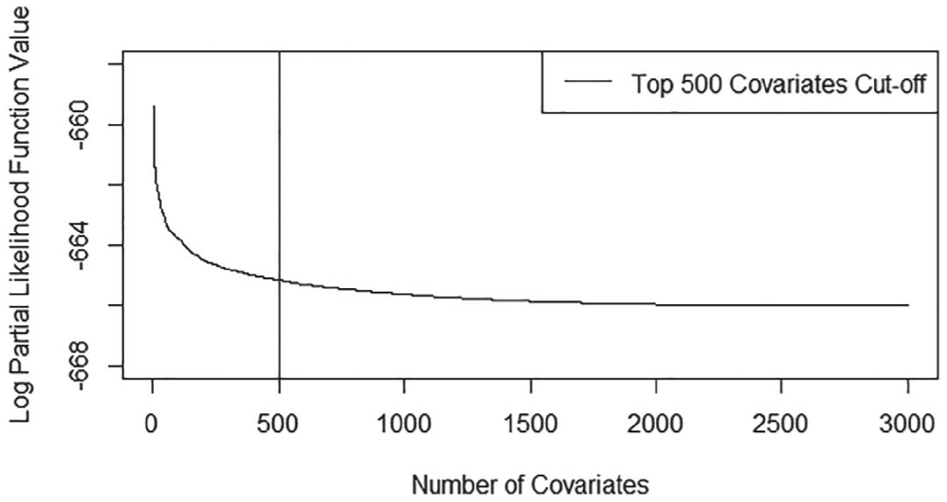
Top 3000 SNPs selected by sure independent screening

TABLE 4.

Variable selection and estimation results for the ADNI data

SNP Name	BAR	LASSO	SCAD	MCP	SELO	SICA
rs10089267	− (–)	− (–)	−0.202(0.155)	−0.186(0.156)	− (–)	− (–)
rs10150971	−0.228(0.189)	− (–)	−0.216(0.178)	−0.251(0.215)	−0.243(0.204)	−0.242(0.212)
rs10165919	− (–)	−0.042(0.084)	−0.228(0.153)	−0.226(0.123)	−0.174(0.144)	−0.170(0.121)
rs1023106	−0.092(0.165)	− (–)	−0.213(0.157)	−0.241(0.145)	−0.192(0.152)	−0.188(0.146)
rs10435804	−0.233(0.282)	− (–)	− (–)	−0.279(0.250)	−0.316(0.231)	−0.319(0.246)
rs10512390	− (–)	− (–)	−0.228(0.177)	− (–)	− (–)	− (–)
rs10513829	−0.149(0.13)	−0.065(0.091)	−0.153(0.150)	− (–)	− (–)	− (–)
rs10520450	− (–)	−0.042(0.090)	− (–)	− (–)	− (–)	− (–)
rs10780472	− (–)	−0.070(0.080)	− (–)	− (–)	− (–)	− (–)
rs10799802	− (–)	−0.067(0.102)	− (–)	− (–)	− (–)	− (–)
rs10821495	− (–)	−0.035(0.065)	− (–)	− (–)	− (–)	− (–)
rs10854810	− (–)	0.011(0.087)	− (–)	− (–)	− (–)	− (–)
rs108609	− (–)	−0.115(0.102)	− (–)	− (–)	− (–)	− (–)
rs11027723	− (–)	−0.046(0.084)	− (–)	− (–)	− (–)	− (–)
rs11131137	− (–)	−0.049(0.079)	− (–)	− (–)	− (–)	− (–)
rs1160728	− (–)	−0.070(0.096)	− (–)	− (–)	− (–)	− (–)
rs11647526	− (–)	−0.13(0.132)	− (–)	− (–)	− (–)	− (–)
rs11704226	− (–)	−0.074(0.091)	− (–)	− (–)	− (–)	− (–)
rs12454238	−0.497(0.134)	−0.329(0.156)	−0.431(0.184)	−0.425(0.138)	−0.441(0.135)	−0.442(0.129)
rs12555515	− (–)	0.040(0.098)	− (–)	− (–)	− (–)	− (–)
rs12589973	− (–)	−0.137(0.109)	− (–)	− (–)	− (–)	− (–)
rs13037957	− (–)	−0.165(0.107)	− (–)	− (–)	− (–)	− (–)
rs1330312	− (–)	− (–)	0.294(0.171)	− (–)	− (–)	− (–)
rs138957	−0.271(0.174)	−0.126(0.068)	− (–)	− (–)	− (–)	− (–)
rs1397228	−0.366(0.139)	−0.124(0.114)	−0.439(0.163)	−0.446(0.132)	−0.433(0.147)	−0.434(0.134)
rs1467025	0.168(0.126)	0.113(0.081)	− (–)	0.196(0.139)	0.165(0.120)	0.161(0.134)
rs1475950	0.793(0.224)	0.045(0.090)	0.888(0.352)	0.878(0.227)	0.816(0.244)	0.814(0.225)
rs1619465	− (–)	0.090(0.103)	− (–)	− (–)	− (–)	− (–)
rs1638438	− (–)	0.052(0.062)	− (–)	− (–)	− (–)	− (–)
rs2050635	− (–)	−0.018(0.11)	− (–)	− (–)	− (–)	− (–)
rs2175859	−0.482(0.199)	−0.033(0.083)	− (–)	−0.553(0.172)	−0.598(0.182)	−0.601(0.171)
rs2428754	0.252(0.211)	0.040(0.088)	− (–)	0.399(0.210)	0.368(0.223)	0.360(0.203)

In Table 4, for each of the 32 SNPs selected by the six penalty functions, the estimated effect is provided along with the estimated standard error in the parentheses obtained by using the bootstrap procedure with 100 bootstrap samples. Among the selected SNPs, only four, rs12454238, rs1397228, rs1475950, and rs2175859, which are located in chromosome 18, 3, 5, and 7, respectively, had significant effects on the AD conversion. In particular, it seems that the presence of allele T in the SNP rs1475950 and the absence of allele T in the SNPs rs12454238, rs1397228, and rs2175859 increased the risk of AD conversion for the subjects with MCI. Figure 4 displays the estimated four nonlinear covariate effects and indicates that higher ADAS13 and MidTemp were related to the increasing risk of the AD conversion. By contrast, lower RAVLT.i and FAQ seem to cause the increasing of the AD conversion risk. The conclusions here are similar to those given by the others who analyzed the same study. On the other hand, it is worth pointing out that most of the previous work only considered a part of the data or performed simplified analyses. For instance, Li et al³⁰ considered only the demographic and clinical factors and Li et al³² and Hu et al³³ performed a single SNP analysis.

FIGURE 4.

Estimated nonlinear covariate effects

To give a graphical idea about the analysis result, Figure 5 presents the estimates of the baseline survival function given by the proposed approach with the use of the six penalty functions mentioned above. One can see from the figure that they are quite close to each other or robust with respect to the penalty function. For comparison, we also obtained the Kaplan-Meier estimate of the general survival function by simplifying the observed data to right-censored data and treating all subjects arising from a homogeneous population and include it in Figure 5 too. It is interesting to see that the Kaplan-Meier estimate is quite close to the model-based estimates for the early period.

FIGURE 5.

Estimated survival functions

6 |. DISCUSSION AND CONCLUDING REMARKS

This article discussed the variable selection and estimation for regression analysis of high-dimensional interval-censored data arising from a partly linear additive Cox model and for the problem, a penalized variable selection procedure was developed and shown through numerical studies to work well for practical situations. In the method, Bernstein polynomials were used to approximate the nonlinear covariate effects as well as the unknown cumulative hazard function. Note that instead of Bernstein polynomials, one can employ other types of polynomials or smooth functions and develop the variable selection methods similarly as above. For the implementation, a coordinate-wise optimization algorithm, which can accommodate most of the existing penalty functions, was developed. The presented approach was then applied to the data from ADNI that motivated this study.

Note that in the proposed variable selection procedure, we used Bernstein polynomials in the sieve approach and it is apparent that a similar method can be developed if one instead employs other smooth functions such as some spline functions. As mentioned above, Zhao et al¹³ considered the same problem discussed here but only for the standard Cox model with linear covariate effects and the situation of p<n. In particular, their optimization algorithm cannot be used for or generalized to high-dimensional covariate situation. This is because it makes use of the Cholesky decomposition of a matrix and involves the inversion of a p×p matrix, which is not only unstable and problematic but also very time consuming when p is very large. By contrast, as shown in the simulation study, the coordinate-wise optimization method given above is much faster for the maximization and can easily handle the high-dimensional (p>n) situation.

There exist several directions for future research. One is that it would be helpful to establish the asymptotic properties of the proposed estimators of the covariate effects as well as the survival function such as their consistency. For this, one needs to deal with several difficulties or factors such as the nonparametric estimation involved and the large p and small p factor. Another direction is that instead of model (1), one may be interested in or prefer to employ the additive Cox model

$$\Lambda (t;X)={\Lambda }_0(t)\text{exp}\{\mathit{\varphi }(X)\}$$

and develop a variable selection and estimation procedure, where $\mathit{\varphi }(X)={\sum }_{j=1}^p{\varphi }_j\left(X_j\right)$ with ϕ_j(X_j) being an unknown function of X_j. It is easy to see that this would be much more challenging than the problem discussed above. To follow the idea above, one possible approach is to approximate the ϕ_j(·)’s by using spline functions or Bernstein polynomials and then to employ some group penalization such as group LASSO.³⁵

In the preceding sections, our focus has been on the main efforts of covariates and sometimes one may be interested in some interaction effects and thus developing the corresponding methods. Although it may seem to be straightforward, the generalization of the proposed method to or development of a method allowing for the selection of interaction effects is nontrivial or not easy.^36–39 Among others, under the current context, one issue that one needs to consider and would affect how a variable selection procedure will be developed is what type of interaction effects from the two sets of covariates considered above are of interest. One choice would be the interaction effects only between low-dimensional covariates and high-dimensional covariates and another would be the interaction effects only among high-dimensional covariates. For the former, one would have to deal with nonlinear interaction effects, which may be quite difficult. For the latter, the problem is relatively easy as one faces linear interaction effects. To deal with it, one may borrow the idea behind the regularization algorithm under marginality principle method discussed in Hao et al,³⁶ who considered the linear model situation.

REFERENCES

- 1.Tibshirani R The lasso method for variable selection in the Cox model. Stat Med. 1997;16:385–395. [DOI] [PubMed] [Google Scholar]
- 2.Fan J, Li R. Variable selection for Cox’s proportional hazards model and frailty model. Ann Stat. 2002;30:74–99. [Google Scholar]
- 3.Cai J, Fan J, Jiang J, Zhou H. Partially linear hazard regression for multivariate survival data. J Am Stat Assoc. 2007;102:538–551. [Google Scholar]
- 4.Zhang H, Lu WB. Adaptive lasso for Cox’s proportional hazards model. Biometrika. 2007;94:1–13. [Google Scholar]
- 5.Bradic J, Fan J, Jiang J. Regularization for Cox’s proportional hazards model with NP-dimensionality. Ann Stat. 2011;39:3092–3120. [DOI] [PMC free article] [PubMed] [Google Scholar]
- 6.Huang J, Liu L, Liu Y, Zhao X. Group selection in the Cox model with a diverging number of covariates. Stat Sin. 2014;24:1787–1810. [Google Scholar]
- 7.Ni A, Cai J. Tuning parameter selection in Cox proportional hazards model with a diverging number of parameters. Scand J Stat. 2018;45:557–570. [DOI] [PMC free article] [PubMed] [Google Scholar]
- 8.Finkelstein DM. A proportional hazards model for interval-censored failure time data. Biometrics. 1986;42:845–854. [PubMed] [Google Scholar]
- 9.Sun J The Statistical Analysis of Interval-Censored Failure Time Data. New York: Springer; 2006. [Google Scholar]
- 10.Wu Y, Cook R. Penalized regression for interval-censored times of disease progression: selection of HLA markers in psoriatic arthritis. Biometrics. 2015;71:782–791. [DOI] [PubMed] [Google Scholar]
- 11.Zhou Q, Hu T, Sun J. A sieve semiparametric maximum likelihood approach for regression analysis of bivariate interval-censored failure time data. J Am Stat Assoc. 2017;112:664–672. [Google Scholar]
- 12.Lu M, McMahan SC. A partially linear proportional hazards model for current status data. Biometrics. 2018;74:1240–1249. [DOI] [PubMed] [Google Scholar]
- 13.Zhao H, Wu Q, Li G, Sun J. Simultaneous estimation and variable selection for interval-censored data with broken adaptive ridge regression. J Am Stat Assoc. 2020;115:204–216. [DOI] [PMC free article] [PubMed] [Google Scholar]
- 14.Kalbfleisch JD, Prentice RL. The Statistical Analysis of Failure Time Data. New York: Wiley; 2002. [Google Scholar]
- 15.Huang J Efficient estimation of the partly linear additive Cox model. Ann Stat. 1999;27:1536–1563. [Google Scholar]
- 16.Du P, Ma S, Liang H. Penalized variable selection procedure for Cox models with semiparametric relative risk. Ann Stat. 2010;38:2092–2117. [DOI] [PMC free article] [PubMed] [Google Scholar]
- 17.Long Q, Chung M, Moreno CS, Johnson BA. Risk prediction for prostate cancer recurrence through regularized estimation with simultaneous adjustment for nonlinear clinical effects. Ann Appl Stat. 2011;5:2003–2023. [DOI] [PMC free article] [PubMed] [Google Scholar]
- 18.Ma S, Du P. Variable selection in partly linear regression model with diverging dimensions for right censored data. Stat Sin. 2012;22:1003–1020. [DOI] [PMC free article] [PubMed] [Google Scholar]
- 19.Scolas S, El Ghouch A, Legrand C, Oulhaj A. Variable selection in a flexible parametric mixture cure model with interval-censored data. Stat Med. 2016;35:1210–1225. [DOI] [PMC free article] [PubMed] [Google Scholar]
- 20.Liu Z, Li G. Efficient regularized regression with L0 penalty for variable selection and network construction. Comput Math Methods Med. 2016;2016:3456153. [DOI] [PMC free article] [PubMed] [Google Scholar]
- 21.Lv J, Fan Y. A unified approach to model selection and sparse recovery using regularized least squares. Ann Stat. 2009;37:3498–3528. [Google Scholar]
- 22.Lin W, Lv J. High-dimensional sparse additive hazards regression. J Am Stat Assoc. 2013;108:247–264. [Google Scholar]
- 23.Tibshirani R Regression shrinkage and selection via the lasso. J R Stat Soc Ser B. 1996;58:267–288. [Google Scholar]
- 24.Fan J, Li R. Variable selection via nonconcave penalized likelihood and its oracle property. J Am Stat Assoc. 2001;96:1348–1360. [Google Scholar]
- 25.Dicker L, Huang B, Lin X. Variable selection and estimation with the seamless-L0 penalty. Stat Sin. 2013;23:929–962. [Google Scholar]
- 26.Zhang CH. Nearly unbiased variable selection under minimax concave penalty. Ann Stat. 2010;38:894–942. [Google Scholar]
- 27.Verweij PJM, Houwelingen HCV. Cross-validation in survival analysis. Stat Med. 1993;12:2305–2314. [DOI] [PubMed] [Google Scholar]
- 28.Schwarz GE. Estimating the dimension of a model. Ann Stat. 1978;6:461–464. [Google Scholar]
- 29.Craven P, Wahba G. Smoothing noisy data with spline functions: estimating the correct degree of smoothing by the method of generalized cross-validation. Numer Math. 1979;31:377–403. [Google Scholar]
- 30.Li K, Chan W, Doody RS, Quinn J, Luo S, Alzheimers Disease Neuroimaging Initiative. Prediction of conversion to Alzheimer’s disease with longitudinal measures and time-to- event data. J Alzheimers Dis. 2017;58:361–371. [DOI] [PMC free article] [PubMed] [Google Scholar]
- 31.Han X, Zhang Y, Shao Y, Alzheimers Disease Neuroimaging Initiative. Application of concordance probability estimate to predict conversion from mild cognitive impairment to Alzheimer’s disease. Biostat Epidemiol. 2017;1:105–118. [DOI] [PMC free article] [PubMed] [Google Scholar]
- 32.Li JQ, Yuan XZ, Li HY, et al. Genome-wide association study identifies two loci influencing plasma neurofilament light levels. BMC Med Genomics. 2018;11:47. [DOI] [PMC free article] [PubMed] [Google Scholar]
- 33.Hu H, Li H, Li J, Yu J, Tan L, Alzheimers Disease Neuroimaging Initiative. Genome-wide association study identified ATP6V1H locus influencing cerebrospinal fluid BACE activity. BMC Med Genet. 2018;19:75. [DOI] [PMC free article] [PubMed] [Google Scholar]
- 34.Fan J, Feng Y, Wu Y. High-dimensional variable selection for Cox’s proportional hazards model. Inst Math Stat Collection. 2010;6:70–86. [Google Scholar]
- 35.Yuan M, Lin Y. Model selection and estimation in regression with grouped variables. J R Stat Soc Ser B. 2006;68:49–67. [Google Scholar]
- 36.Hao N, Feng Y, Zhang HH. Model selection for high-dimensional quadratic regression via regularization. J Am Stat Assoc. 2018;113:615–625. [Google Scholar]
- 37.Bien J, Taylor J, Tibshirani R. A lasso for hierarchical interactions. Ann Stat. 2013;41:1111–1141. [DOI] [PMC free article] [PubMed] [Google Scholar]
- 38.Choi NH, Li W, Zhu J. Variable selection with the strong heredity constraint and its oracle property. J Am Stat Assoc. 2010;105:354–364. [Google Scholar]
- 39.Zhao P, Rocha G, Yu B. The composite absolute penalties family for grouped and hierarchical variable selection. Ann Stat. 2009;37:3468–3497. [Google Scholar]