Hypothesis testing for phylogenetic composition: a minimum-cost flow perspective

Summary

Quantitative comparison of microbial composition from different populations is a fundamental task in various microbiome studies. We consider two-sample testing for microbial compositional data by leveraging phylogenetic information. Motivated by existing phylogenetic distances, we take a minimum-cost flow perspective to study such testing problems. We first show that multivariate analysis of variance with permutation using phylogenetic distances, one of the most commonly used methods in practice, is essentially a sum-of-squares type of test and has better power for dense alternatives. However, empirical evidence from real datasets suggests that the phylogenetic microbial composition difference between two populations is usually sparse. Motivated by this observation, we propose a new maximum type test, detector of active flow on a tree, and investigate its properties. We show that the proposed method is particularly powerful against sparse phylogenetic composition difference and enjoys certain optimality. The practical merit of the proposed method is demonstrated by simulation studies and an application to a human intestinal biopsy microbiome dataset on patients with ulcerative colitis.

1. Introduction

High-throughput sequencing technologies make it possible to survey the microbiome communities from multiple samples, resulting in a need for statistical methods to quantitatively compare samples from different populations/experiments. Testing whether two groups of samples have the same microbiome composition is a key step in deciphering the quantitative difference between populations and identifying the dysbiotic components. In this paper we consider two-sample testing for the means of relative abundance from two populations. Although the problem is mainly motivated by microbiome and metagenomic data analysis, as a general problem it also arises in other high-throughput sequencing data, e.g., single-cell RNA sequencing data.

The microbial community from one sample is usually represented by discrete distributions with the relative abundance of microbe species organized in taxonomy, or operational taxonomic units in some applications. To assess the quantitative difference between groups of samples, various methods have been proposed for the taxonomic compositional data, including global two-sample tests (Zhao et al., 2015; Cao et al., 2017) and differential abundance tests (Robinson et al., 2010; Wagner et al., 2011; Love et al., 2014; Mandal et al., 2015). These methods, however, neglect the degree of similarity between microbe species, due to the fact that the analysis units in these methods, microbe species, are implicitly assumed to be equally distinct (Fukuyama, 2017). Furthermore, the classification of microbes by contemporary microbial taxonomy is coarse, which results in loss of power to detect subtle difference in a higher resolution (Washburne et al., 2018). To alleviate these issues, the phylogeny of the bacterial species is usually incorporated into the analyses of microbiome data (Fukuyama, 2017; Washburne et al., 2018).

In order to capture the phylogenetic compositional difference of the microbes between populations, one of the most widely used two-sample testing methods is multivariate analysis of variance with permutation, permanova, equipped with phylogenetic distance (McArdle & Anderson, 2001; Anderson, 2014; Xia & Sun, 2017). In microbiome data analysis, the popular choices of phylogenetic distances include the unweighted or weighted UniFrac distances (Lozupone & Knight, 2005; Lozupone et al., 2007) and their Zolotarev-type generalized variants (Evans & Matsen, 2012). Through studying these phylogenetic composition distances, we show that they are closely related to a minimum-cost flow problem for the underlying phylogenetic tree, and the phylogenetic composition difference between samples can be fully characterized by the optimal flow at each edge. Motivated by this observation, we consider the optimal flow at each edge as the analysis unit, instead of each microbe species. The main goal of the present paper is to study the problem of two-sample testing on a phylogenetic tree from this minimum-cost flow perspective.

We first investigate permanova equipped with Zolotarev-type phylogenetic distance. Due to its flexibility and ease of computation, permanova using phylogenetic distance has been applied in a wide range of microbiome studies (Smith et al., 2015; Chen et al., 2016; Wu et al., 2016), but it still lacks theoretical justification. Following the minimum-cost flow perspective, we show that permanova is essentially a sum-of-squares type of test, which has been widely used to test the difference between the means of two populations in high-dimensional problems (Bai & Saranadasa, 1996; Srivastava & Du, 2008; Chen & Qin, 2010). We establish its asymptotic normality under the null hypothesis, and show that its power is indeed determined by the phylogenetic distance between the group means. It is known that sum-of-squares type tests are effective in detecting the dense alternatives, but not powerful against sparse alternatives (Cai et al., 2014; Chen et al., 2019). However, in most microbiome studies, only a small fraction of taxa may have different mean abundances (Cao et al., 2017), resulting in optimal flows on a small number of edges that are active, i.e., nonzero. Moreover, permanova, as a global method, is not able to identify the specific locations of the significant differences even when the null hypothesis is rejected. Therefore, there is a need for a more powerful and interpretable test to detect sparse phylogenetic composition difference between two populations.

To fill this need we introduce a new test, detector of active flow on the tree, dafot, to detect the sparse phylogenetic composition difference between two populations. To detect sparse signals, the maximum type statistics are usually adopted in various settings because of their simplicity, effectiveness and optimality (see, e.g., Dümbgen & Spokoiny, 2001; Arias-Castro et al., 2005; Jeng et al., 2010; Arias-Castro et al., 2011; Cai et al., 2014, and references therein). Motivated by this, we construct dafot as the maximum of the standardized statistics for optimal flow at each edge. When the null hypothesis is rejected by dafot, it is also able to identify the edges that the active optimal flows lie on. Thus, different from permanova, dafot can not only detect the difference, it is also able to identify the branches of the phylogenetic tree that show difference in relative abundance between the populations. It is shown that dafot is the minimax optimal test against sparse alternatives, and the optimal detection boundary of phylogenetic composition difference relies on both the structure of phylogenetic tree and heteroskedastic variance of microbe species. The practical merits of dafot are further demonstrated through a real data example. The method is implemented in the R package DAFOT available from CRAN (R Development Core Team, 2021).

Transformation of compositional data is often employed in order to account for the compositional nature of the data. For example, the centred log-ratio transformation is one of the commonly used transformation methods for analysis of compositional data (Aitchison, 1982). To account for possible data transformation, we introduce -generalized optimal flow for any given strictly increasing transformation function defined on . The original form of optimal flow corresponds to the special case with . Another special case of -generalized optimal flow is the difference of balance between populations (Egozcue & Pawlowsky-Glahn, 2016; Rivera-Pinto et al., 2018), when , equivalent to adopting centred log-ratio transformation. After introducing this new concept, we show that all the methodology and theory discussed previously can be generalized accordingly.

2. A hierarchical model for microbiome count data and phylogenetic distance

The human microbiome can be quantified using 16S rRNA sequencing or shotgun metagenomic sequencing. Such 16S rRNA gene sequences of the bacterial genomes or the sequencing of evolutionarily conserved universal marker genes can be used to construct the phylogenetic tree of the bacterial species. The microbe species and their ancestors are usually organized in such a phylogenetic tree based on their evolutionary relationships. Let be the phylogenetic tree of microbe species. Here, is the collection of microbe species and their ancestors, and represents the collection of edges of the phylogenetic tree . For any , is the corresponding branch length. We assume the phylogenetic tree is rooted at , which can be seen as the common ancestor of all microbe species. For any pair of nodes , the unique shortest path between them is denoted by and the corresponding distance between them is defined as

(1)

The dissimilarity between two microbe species and can thus be quantified by . The height of the tree is then defined as the maximum of the distances between the root and the other nodes of the tree, .

The relative abundance of a microbial community can be represented by a discrete distribution on the nodes of the tree . More specifically, write all possible discrete distributions on as

Here, is the relative abundance of microbial species and is a simplex of dimension, where is the number of elements. Suppose there are two populations of interest on , e.g., treated and control groups. These two populations can be represented by two probability distributions on , and , respectively. We are interested in comparing the mean of the relative abundance between these two populations,

(2)

where is the mean of ,

The covariance matrix of is defined similarly:

To test the mean equality hypothesis, and samples are drawn from each of the two populations,

However, the true relative abundance of each sample, , , , is unknown in practice. Sequencing of the microbial DNAs is used to assess the relative abundance of the microbes in the sample. In microbiome studies, the sequencing read data can be modelled by a Poisson distribution. To be specific, the number of sequencing reads that can be assigned to species from the th sample of the th group is assumed to follow a Poisson distribution,

where is the total number of reads in the th sample of the th group and is the relative abundance of microbe species in sample . Thus, the reads count is assumed to be drawn from the hierarchical model

for any , , . The goal of this paper is to test the hypothesis in (2) based on the count data .

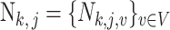Following this hierarchical model, the empirical distribution of each is written as 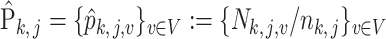. Due to the hierarchical structure of the model, the covariance matrix of empirical distribution is

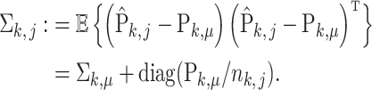Here, represents the diagonal matrix of a vector. It is clear that the covariance matrix of the empirical distribution depends on both the mean and covariance matrix of , and the variance of the empirical distribution is inflated because of the sequencing steps. The difference between and vanishes when goes to infinity. For simplicity of analysis, in the rest of the paper we always assume the total number of reads in each sample to be equal, i.e., for any , . For brevity, we write when and . We also assume that there exists such that

(3)

This assumption implies that the proportion of the samples from either population does not vanish. We write .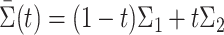

In microbiome studies, a phylogenetic distance that reflects the evolution relationships among microbe species is often used in defining the distance between two microbial communities. Examples include unweighted and weighted UniFrac distance (Lozupone & Knight, 2005; Lozupone et al., 2007). As shown in Evans & Matsen (2012), the weighted UniFrac distance is a plugin estimator of the Wasserstein distance of probability masses on the tree, which can be generalized to Zolotarev-type variants; for brevity, we call them Zolotarev-type phylogenetic distance. In the present paper we focus on the Zolotarev-type phylogenetic distance

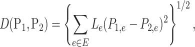(4)

where is the total probability of all descendants of edge ,

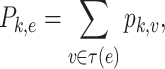where and is a subtree below edge : . We also use the following notation:

3. A minimum-cost flow perspective for two-sample testing

The phylogenetic distance between two discrete distributions is closely related to optimal transport theory (Evans & Matsen, 2012). To be specific, the weighted UniFrac/Wasserstein distance between and is equal to the solution of the following optimal transport problem:

(5)

Here, the objective function is the total cost of transport , and is the cost per unit transported from to .

Different from the general optimal transport problem, the distance in (1) is defined as the geodesic distance along the path on tree . Therefore, this optimal transport problem can be naturally cast as a minimum-cost flow problem on a network, as illustrated in Fig. 1. The tree can be seen as a special network, and there is a source with capacity and a sink with capacity at each node . Then, the optimization problem in (5) aims to find a way with the minimum cost of sending an amount of flow from sources to sinks through the network . In particular, for any given transport 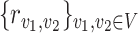, define the flows on each edge as

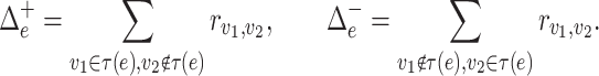Figure 1.

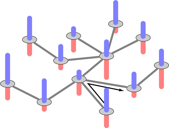
An illustration of the minimum-cost flow problem on the tree. The blue bars are the source and the red bars are the sink.

Here, is the flow through edge towards the root , and is the flow through edge in the opposite direction. Then, the optimization problem in (5) can be reformulated as

(6)

Although the optimal transport in (5) might not be unique, the optimal flow in (6) is unique and has the closed-form solution

The optimal net flow on each edge is then defined as 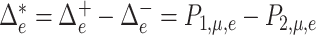. The weighted UniFrac distance and corresponding Zolotarev-type variants can thus be seen as the weighted norm of optimal flows. It is clear from the above discussion that the phylogenetic composition difference between and can be fully characterized by the optimal flow . If we write , the hypothesis in (2) can be rewritten in the equivalent form

This suggests that the basic unit to quantify phylogenetic composition difference shall be the optimal flow at each edge . The Zolotarev-type phylogenetic distance can be seen as the norm of these optimal flows.

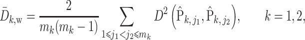
4. Permutational multivariate analysis of variance

4.1. Introduction

To incorporate phylogenetic tree information in comparing two populations, one of the most commonly used two-sample tests is permanova equipped with some phylo-genetic distance (McArdle & Anderson, 2001; Anderson, 2014). Specifically, let be the phylogenetic distance defined in (4). The average empirical distances within and between groups are defined as

and

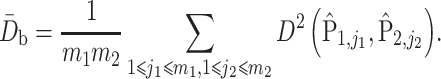Similar to analysis of variance, permanova defines the total sum-of-squares as

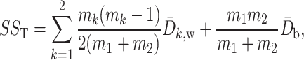and the within-group sum-of-squares and between-group sum-of-squares as

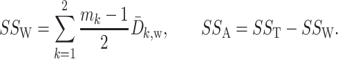The pseudo -statistic for two-sample testing is then defined as the normalized ratio of to ,

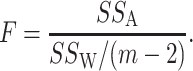To evaluate the significance of the -statistic, its -value is calculated by permutations. To be more specific, the samples are permuted randomly times and the -statistic calculated on each of these permuted data, denoted . Then, the estimated -value is

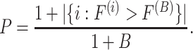One implicit assumption of a valid permutation test is the exchangeability of samples under the null hypothesis. Thus, the hypothesis required by a valid permutation test is

Compared with the mean equality hypothesis in (2), this is a more restrictive hypothesis. In the next section we present another way to estimate the -value of permanova based on the asymptotic results.

4.2. Properties

We investigate the properties of the pseudo -statistic under the Zolotarev-type phylogenetic distance . A simple calculation decomposes into two parts:

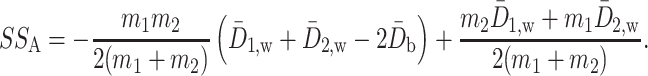In particular, the second term is asymptotically equal to ,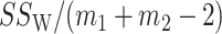

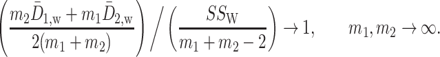This shows that is a scaled version of the difference between the average within-group distance and the across-group distance. In other words, in terms of two-sample testing, is asymptotically equivalent to the following energy distance statistic (Székely & Rizzo, 2005; Sejdinovic et al., 2013):

Due to the fact that the distance in (4) is a negative type, the energy distance statistic can also be written as a kernel-based test statistic (Sejdinovic et al., 2013),

where the kernel of and is defined as . The kernel form of permanova suggests

Therefore, the statistic in permanova is a reasonable statistic for testing the phylogenetic composition difference in hypothesis (2), as the mean of only depends on and .

Clearly, the behaviour of depends on both the covariance matrix of and the tree structure . The structure of the tree can be expressed as a transformation matrix , where if and if . We assume

(7)

where or . Such a moment assumption is a common condition in high-dimension statistics, e.g., condition (3.6) in Chen & Qin (2010). Condition (7) is true when the eigenvalues of both and are bounded. Besides the assumption of the moment, another assumption we make is

(8)

where and are empirical distributions drawn from the first or second population, and is a sequence of numbers such that . This is a fairly weak condition. For example, it is a trivial assumption when the tree is not too high, i.e., , because .

The following theorem shows the asymptomatic behaviour of the permanova statistic .

Theorem 1.

Under the null hypothesis, i.e., , and assumptions (3), (7) and (8),

 where can be written as  

Furthermore, if and assumptions (3), (7) and (8) hold, the test is consistent when  

(9)

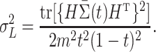
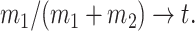
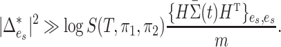
This theorem suggests that permanova is a consistent test if the phylogenetic distance between the means of two populations is large enough. As can be written explicitly as

the power of permanova depends on both the number of samples and the number of reads per sample . The power becomes larger if we increase either or . However, (9) also suggests that a larger number of samples is a more efficient way to increase power than a larger number of reads per sample. This theorem also suggests that the -value can be calculated based on asymptomatic distribution instead of conducting permutations. For instance, can be estimated based on a similar -statistic, in Chen & Qin (2010). Then, the -value can be calculated by . This way of calculating the -value does not require under the null hypothesis. In practice, we recommend the permutation test when is not large and the asymptotic critical value of is large.

4.3. Sparse setting

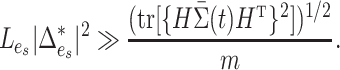
As we have seen in previous sections, permanova is a sum-of-squares type statistic. However, the interesting setting in practice, e.g., in microbiome studies, is a sparse case where only a small number of microbe species may have different relative mean abundance (Cao et al., 2017). This suggests that only a small fraction of optimal flow is active, i.e., . To investigate the performance of permanova under this sparse setting, we consider a simple case where there is active optimal flow on one edge, denoted by . As suggested by Theorem 1, the condition for a consistent permanova test is

On the other hand, we consider an oracle test that has knowledge of the active flow location . Since the location of is known, we consider a two-sample -test for ,

(10)

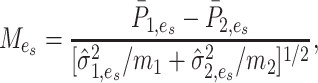
where

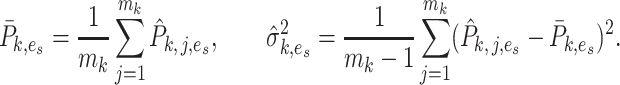With the central limit theorem, we know that is a consistent test if

A comparison of the two detection boundaries indicates that the oracle test is able to detect a much smaller difference between two groups of samples than permanova. This naturally leads to the question of whether it is possible to develop a more powerful test under the sparse flow setting.

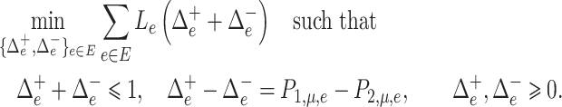
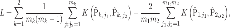
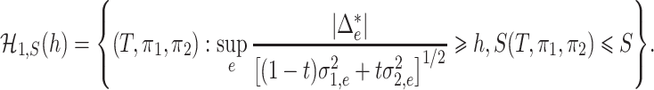
5. Active optimal flow detection

5.1. Detector of active flow on the tree

As shown in § 4, the two-sample -test could improve the power to detect the difference between two populations when the location of the active optimal flow is known. In practice, the location information is usually unknown. To address this issue we consider the maximum of the two-sample -tests at each edge,

where is defined in the same way as (10). The use of this maximum type statistic for detecting sparse signals is very common in a wide range of applications, leading to the construction of rate-optimal tests for many problems (Dümbgen & Spokoiny, 2001; Arias-Castro et al., 2005; Arias-Castro et al., 2011; Jeng et al., 2010; Cai et al., 2014; Cao et al., 2017; Wang et al., 2021).

To evaluate the statistical significance of , one still needs to choose an appropriate critical value for . However, it is difficult to derive the asymptotic distribution of due to the complex dependency structure among the . To overcome this problem, one adopts a resampling method to assign an appropriate critical value for . In particular, a common resampling method to choose a critical value is the permutation test as in permanova (Good, 2013; Anderson, 2014). Although the permutation test requires under the null hypothesis as we discussed before, its performance is robust when the sample size is small.

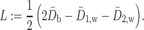
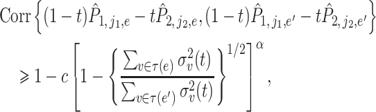
We propose another resampling method, the bootstrap, to choose the critical value for in order to avoid the condition . Let for , , where is the mean of within each group and is the mean of the combined samples. We randomly draw samples with replacement from each group and then calculate with shifted data . This procedure is repeated times and the corresponding statistics are denoted by . Finally, the approximated is chosen as a quantile of the empirical distribution of , or the -value is calculated as

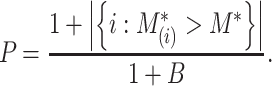We then make a decision under the null hypothesis based on the critical value or the -value.

When the null hypothesis is rejected, also provides a natural way to identify the set of edges with their optimal flow not being zero, . To be specific, we consider the set of edges as the active edges identified. Due to the construction of , the familywise error rate of active edge identification is naturally controlled at the level. The identified edge indicates that all microbe species below this edge, as a whole object, are differentially abundant between the two populations. In this way, the active edges are identified as a microbial signature associated with the difference of the two populations.

5.2. Asymptotic behaviour and optimality of

We now investigate the behaviour of under the null and alternative hypothesis. The main difficulty in studying the behaviour of is the strong and complex dependence among different . This complexity of the dependency structure mainly comes from two sources: the high overlapping structure of the subtree and the unknown heteroskedastic variance/covariance structure among the different microbe species. Our investigation shows that the complexity of the the dependence structure among the can be characterized by a single quantity that depends on both the tree structure and the heteroskedastic variance.

Since each is defined on a subtree below edge , the asymptotic behaviour of clearly depends on the effective number of subtrees. We still assume that each group of samples has no vanishing proportion, i.e., (3). Let be the element of the th row and th column of . To decouple the complex dependence structure among the , we provide the following proposition.

Proposition 1.

For any given , let be a subset of edges of the tree such that . Then, can be decomposed into a collection of disjoint paths  

 where and are nodes of the tree and is the number of disjoint paths. In addition, any two edges from different paths in the above decomposition do not share any descendants.

Intuitively, for any and from the same path defined above, the subtrees and are highly overlapped, and thus the defined on them are expected to behave similarly. On the other hand, for edges from different paths, the corresponding subtrees are distinct in that they do not share any descendants. In general, the number of disjoint paths in the above proposition characterizes an effective number of subtrees. Motivated by this observation, we define as the number of different paths in for , and as the sum of the ,

Clearly, is an integer between and , and depends on the structure of the tree and the distributions and . For example, when the tree is a fully balanced binary tree, and and are Dirichlet distributions with equal parameters for the leaves, . If and are Dirichlet distributions with equal parameters for all nodes of a chain tree , i.e., a one-dimensional lattice, then . More specific examples can be found in the Supplementary Material. We later show that the asymptotic behaviour of can be fully characterized by this quantity .

When two subtrees highly overlap, we expect the correlation between the on them to be very strong. We shall assume there exist constants and such that

(11)

where , and are a pair of edges such that . Here, represents the correlation between two random variables. This is not a strong condition. For instance, (11) is satisfied when the relative abundance of different microbe species in are mutually independent or drawn from a Dirichlet distribution. Furthermore, we also assume that is a sub-Gaussian distribution, i.e., there exist constants and such that

(12)

where is the variance of , the element of the th row and the th column of . The following theorem shows the asymptotic behaviour of under the null hypothesis.

Theorem 2.

Suppose . Under the null hypothesis and assumptions (3), (11) and (12), we have  

(13)

Theorem 2 suggests that the amplitude of is when the null hypothesis is true, where plays the same role as the number of variables when all the components are almost independent (Cai et al., 2014; Cao et al., 2017). In other words, although is constructed from different subtrees, it is equivalent to taking a maximum of roughly independent variables because of the high dependency among the statistics . For the one active flow example discussed in the previous section, Theorem 2 suggests that is a consistent test when

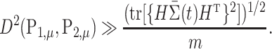
A comparison between the above and the oracle test’s detection boundary suggests that the price we pay for the unknown location of is . With the same argument as for permanova, we know that either a larger number of samples or a larger number of reads per sample can increase the power of dafot. More detailed discussions are given in § 6.

We next turn to the power analysis of the test based on from a minimax point of view (Ingster 1993a, b,c; Ingster & Suslina, 2012). The parameter space of the null hypothesis is

and the parameter space of the alternative hypothesis is

The worst-case risk of any given test is then defined as

We say a test is consistent for separating and if , and and are separable if there exists a consistent test for them. On the other hand, a test is powerless for separating and if , and and are inseparable if . Here, is a parameter to control the distance between and . Clearly, if is smaller, and are more difficult to separate. Let be the test that rejects the null hypothesis if and only if for some . The following theorem characterizes the power of and the separability of and .

Theorem 3.

Consider testing and by . Suppose , and (3), (11) and (12) hold. Then there exist constants and such that  

This theorem shows that the optimal rate of detection boundary between and is

This optimal rate suggests that the difficulty of this problem is mainly determined by the single quantity , which relies on both the tree structure and the heteroskedastic variance structure. This theorem also suggests that is minimax rate optimal.

6. Numerical experiments

6.1. Simulation studies

We investigate the properties of permanova and dafot using simulated datasets. We choose a phylogenetic tree of bacteria species within the class Gammaproteobacteria as the underlying tree . This tree is extracted from the reference tree of the Greengenes 16S rRNA database version 13.8 clustered at 85% similarity by the R package metagenomeFeatures (DeSantis et al., 2006), and has a total of 247 leaves, denoted by , and 246 internal nodes, denoted by . Figure 2 shows the structure of the tree, with each leaf labelled with a number.

Figure 2.

Phylogenetic tree of bacteria within the class Gammaproteobacteria used in the simulation studies, with each leaf node labelled with a number. The edges with active optimal flow in the numerical examples are shown in red.

To simulate the numbers of reads on this tree , we adopt the Dirichlet-multinomial distribution. More specifically, the true relative abundance , where and , is drawn from some Dirichlet distribution, i.e., follows a Dirichlet distribution indexed by ,

For each sample, the reads are then drawn from a multinomial distribution with respect to the true relative abundance. Under this model, the mean of the relative abundance for the th group can be written as

Thus, under the null hypothesis, we assume if and if . Under the alternative hypothesis, we perturb and consider two different scenarios: (A) the difference is at nodes and , i.e., and ; (B) the difference is at clades and , i.e., if and if . The parameter is specified later. In particular, the edges with active optimal flow under scenarios (A) and (B) are shown in red in Fig. 2.

The first set of simulation experiments are designed to compare the performance of dafot and permanova under scenario (A). To be specific, we compare four different methods: dafot; dafot after centre log-ratio transformation (dafot-log); permanova equipped with the weighted UniFrac distance (permanova-L1); and permanova equipped with the Zolotarev-type phylogenetic distance (permanova-L2). To make the comparisons fair, the critical values for all tests are chosen by permutations at a significance level of . To investigate the effect of the sample size , the sequence depth and the signal strength , we chose , and , and , and , , , , and in the simulation experiments. The experiment is repeated 100 times for each combination of the , and . The performance of the tests is evaluated by the power of the test, i.e., the probability of rejecting the null hypothesis, which can be estimated by the proportion of null hypothesis rejections among the 100 simulation experiments.

The results are summarized in Fig. 3. These results show that the Type I error is under control when the null hypothesis is true, , and the power of dafot is larger than permanova when the alternative hypothesis is true (). Figure 3 implies that the observed effects of , and on the power of the tests are consistent with the theoretical results. We observe a similar improved power of dafot over permanova for scenario (B) when the active flows connect two clades; see the Supplementary Material for details.

Figure 3.

Power comparisons between dafot and permanova under scenario (A), where the difference is at nodes and . dafot, the proposed method based on proportions; dafot-log, the proposed method based on log-proportions permanova-L1, permanova with the Zolotarev-type phylogenetic distance; permanova-L2, permanova with the Zolotarev-type phylogenetic distance.

The sequence count data in real microbiome studies are usually very sparse, i.e., there are a lot of zero values. The next set of simulation experiments are designed to assess the performance of dafot and permanova when there are a lot of zero values. More concretely, we set for under scenario (A) and for under scenario (B). In other words, the probability on nearly of the nodes is zero in scenario (A), and the probability on nearly of the nodes is zero in scenario (B). In order to avoid undefined values of , zero counts are replaced by in dafot-log (Aitchison, 2003; Lin et al., 2014). The sequence depth of each sample is drawn uniformly between and instead of being fixed as in previous experiments. The sample size and the difference between populations are varied in the same way as in the previous simulation experiments. We present the results based on 100 runs for each combination of and in the Supplementary Material. A comparison suggests that dafot, permanova-L1 and permanova-L2 are relatively robust against a lot of zero values; however, the power of dafot-log is affected by these zero values.

We further compare the performance of dafot and permanova under a wide range of sparseness. Specifically, we adopt a similar setting to scenario (A) and choose , and . To assess the effect of sparsity, we randomly choose leaves at each simulation experiment and set for the first leaves and for the last leaves; is chosen to be , , , , , and . The results based on 100 simulation experiments are summarized in Fig. 4. These results show that dafot outperforms permanova when fewer leaves are perturbed. When the signal becomes denser, permanova-L1 can gain more power than dafot.

Figure 4.

Power comparisons between dafot and permanova for different sparsity levels.

The final set of simulation experiments aims to evaluate the performance of edge identification by dafot and dafot-log. In particular, we consider scenario (A) with and vary and as in the previous simulation experiments. For each combination of and , we repeat the experiment 100 times and the active edges detected by the two methods are recorded. The results of the average number of false positive edges, the probability of making at least one Type I error, and the true positive edges are summarized in Table 1, showing that the familywise error rate is under control regardless of signal strength, and that the two active edges can be identified successfully when the signal is strong enough. In Fig. 3 and Table 1, dafot-log performs better than dafot, as the log transformation is suitable for nonzero data.

Table 1.

The edge identification performance of dafot and dafot-log

dafot	afp		0.09	0.06		0.08	0.13		0.10	0.08
	fwer		0.04	0.06		0.06	0.09		0.10	0.06
	atp		0.11	0.15		0.56	0.78		1.49	1.66
dafot-log	afp		0.08	0.05		0.08	0.13		0.13	0.36
	fwer		0.04	0.05		0.07	0.11		0.05	0.21
	atp		0.35	0.50		0.90	1.35		1.81	1.94

afp, the average number of false positive edges; fwer, the probability of making at least one Type I error; atp, the number of true positive edges.

6.2. Analysis of ulcerative colitis disease microbiome data

To further demonstrate the performance of dafot, we apply the method to a 16S rRNA dataset of 47 human intestinal biopsy samples collected at the University of Pennsylvania. These samples are divided into three groups: A, 18 control samples (control); B, 14 samples with ulcerative colitis who did not receive treatment (unexposed); C, 15 samples with ulcerative colitis who received treatment (exposed). To compare the microbiome communities of these groups, the raw sequence reads of each sample are placed into a reference phylogenic tree from Greengenes 16S rRNA database version 13.8 with a 99% similarity by using sepp (Mirarab et al., 2012; Janssen et al., 2018). The reference phylogenetic tree is then trimmed by keeping all nodes related to the operational taxonomic units observed in the samples. The trimmed phylogenetic tree is shown in Fig. 5(a), including 7980 edges. Figure 5(b) shows the empirical optimal flow between groups A and B on each edge, i.e., the difference of probability on subtrees indexed by edges, . The order of the edges is ranked automatically by the R class phylo. It is clear from Fig. 5(b) that most of the empirical active flows are small, indicating that sparse flow on the tree is a reasonable assumption. In addition, we estimate the effective number of subtrees for pairwise comparison: for groups A and B; for groups A and C; 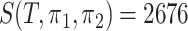for groups B and C. The estimation of is based on the reference phylogenetic tree structure and estimated variance at each node .

Figure 5.

(a) The reference phylogenetic tree used in analysis of intestinal biopsy samples. The branches in red are those identified as an active edge and the zoomed-in subtree below the active edge. (b) The empirical optimal flow between group A and group B on each edge.

To test the phylogenetic composition difference between the groups, we apply the same four two-sample testing methods as in the first simulation experiment. The resulting -values estimated by a permutation test with 1000 permutations are summarized in Table 2. No methods identify any significant phylogenetic composition difference between groups C and A or groups C and B, . However, only dafot indicates an overall difference in intestinal biopsy microbiome composition between groups A and B with , while the other methods do not detect such a difference.

Table 2.

The -values for comparing different groups using dafot and permanova based on 1000 permutations

	dafot	dafot-log	permanova-L1	permanova-L2
Group A vs B	0.007	0.256	0.378	0.460
Group A vs C	0.147	0.495	0.305	0.270
Group B vs C	0.648	0.832	0.639	0.677

Besides the overall difference in microbiome compositions between groups A and B, dafot also identifies that the overall difference is due to the active flow on one edge. The subtree indexed by this edge is shown in Fig. 5(a), coloured red in the original phylogenetic tree and zoomed-in in a side figure. There are a total of 31 operational taxonomic units placed on this subtree, 18 of which are annotated as the Ruminococcaceae family and Oscillospira genus, and 13 of which are annotated as the Ruminococcaceae family and unknown genus. Figure 6(a) shows a boxplot of the combined relative abundance on these 31 operational taxonomic units, indicating that the relative abundance on this subtree decreased in ulcerative colitis patients, but is increased partially after receiving treatment. This is consistent with the previous findings on the proportion of Oscillospira genus and the Ruminococcaceae family in gut microbiota deceases in inflammatory bowel disease patients (Morgan et al., 2012; Konikoff & Gophna, 2016; Santoru et al., 2017). For comparison, a boxplot of the combined relative abundance of all operational taxonomic units assigned to the Oscillospira genus is shown in Fig. 6(b), showing that the pattern of relative abundance found in Fig. 6(a) is not that clear any more. This suggests that the finer species classification by microbial phylogeny can provide more power to detect the subtle difference between populations than standard taxonomic classification (Washburne et al., 2018).

Figure 6.

Boxplots of relative abundance on operational taxonomic units placed on the detected subtree in Fig. 5(a) and on all operational taxonomic units assigned to the Oscillospira genus. The red dots show the raw relative abundance.

Supplementary material

Supplementary material available at Biometrika online includes proofs of all theorems, additional simulation results and information on generalized optimal flow. The software package dafot is available at https://cran.r-project.org/web/packages/DAFOT/index.html.

References

- Aitchison, J. (1982). The statistical analysis of compositional data. J. R. Statist. Soc. B 44, 139–60. [Google Scholar]
- Aitchison, J. (2003). The Statistical Analysis of Compositional Data. Caldwell, NJ: Blackburn Press. [Google Scholar]
- Anderson, M. J. (2014). Permutational multivariate analysis of variance (PERMANOVA). Wiley Statsref, doi: 10.1002/9781118445112.stat07841. [DOI] [Google Scholar]
- Arias-Castro, E., Candes, E. J. & Durand, A. (2011). Detection of an anomalous cluster in a network. Ann. Statist. 39, 278–304. [Google Scholar]
- Arias-Castro, E., Donoho, D. L. & Huo, X. (2005). Near-optimal detection of geometric objects by fast multiscale methods. IEEE Trans. Info. Theory 51, 2402–25. [Google Scholar]
- Bai, Z. & Saranadasa, H. (1996). Effect of high dimension: By an example of a two-sample problem. Statist. Sinica 6, 311–29. [Google Scholar]
- Cai, T. T., Liu, W. & Xia, Y. (2014). Two-sample test of high-dimensional means under dependence. J. R. Statist. Soc. B 76, 349–72. [Google Scholar]
- Cao, Y., Lin, W. & Li, H. (2017). Two-sample tests of high-dimensional means for compositional data. Biometrika 105, 115–32. [Google Scholar]
- Chen, J., Ryu, E., Hathcock, M., Ballman, K., Chia, N., Olson, J. E. & Nelson, H. (2016). Impact of demographics on human gut microbial diversity in a US midwest population. PeerJ 4, e1514. [DOI] [PMC free article] [PubMed] [Google Scholar]
- Chen, S., Li, J. & Zhong, P. (2019). Two-sample and ANOVA tests for high-dimensional means. Ann. Statist. 47, 1443–74. [Google Scholar]
- Chen, S. & Qin, Y. (2010). A two-sample test for high-dimensional data with applications to gene-set testing. Ann. Statist. 38, 808–35. [Google Scholar]
- DeSantis, T. Z., Hugenholtz, P., Larsen, N., Rojas, M., Brodie, E. L., Keller, K., Huber, T., Dalevi, D., Hu, P. & Andersen, G. L. (2006). Greengenes, a chimera-checked 16S rRNA gene database and workbench compatible with ARB. Appl. Environ. Microbiol. 72, 5069–72. [DOI] [PMC free article] [PubMed] [Google Scholar]
- Dümbgen, L. & Spokoiny, V. G. (2001). Multiscale testing of qualitative hypotheses. Ann. Statist. 29, 124–52. [Google Scholar]
- Egozcue, J. J. & Pawlowsky-Glahn, V. (2016). Changing the reference measure in the simplex and its weighting effects. Austrian J. Statist. 45, 25–44. [Google Scholar]
- Evans, S. & Matsen, F. (2012). The phylogenetic Kantorovich–Rubinstein metric for environmental sequence samples. J. R. Statist. Soc. B 74, 569–92. [DOI] [PMC free article] [PubMed] [Google Scholar]
- Fukuyama, J. (2017). Adaptive gPCA: A method for structured dimensionality reduction. arXiv: 1702.00501. [Google Scholar]
- Good, P. (2013). Permutation Tests: A Practical Guide to Resampling Methods for Testing Hypotheses. New York: Springer Science & Business Media. [Google Scholar]
- Ingster, Y. I. (1993a). Asymptotically minimax hypothesis testing for nonparametric alternatives I. Math. Meth. Statist. 2, 85–114. [Google Scholar]
- Ingster, Y. I. (1993b). Asymptotically minimax hypothesis testing for nonparametric alternatives II. Math. Meth. Statist. 2, 171–89. [Google Scholar]
- Ingster, Y. I. (1993c). Asymptotically minimax hypothesis testing for nonparametric alternatives III. Math. Meth. Statist. 2, 249–68. [Google Scholar]
- Ingster, Y. I. & Suslina, I. A. (2012). Nonparametric Goodness-of-Fit Testing under Gaussian Models, New York: Springer Science & Business Media. [Google Scholar]
- Janssen, S., McDonald, D., Gonzalez, A., Navas-Molina, J. A., Jiang, L., Xu, Z., Winker, K., Kado, D. M., Orwoll, E., Manary, M. et al. (2018). Phylogenetic placement of exact amplicon sequences improves associations with clinical information. MSystems 3, e00021. [DOI] [PMC free article] [PubMed] [Google Scholar]
- Jeng, X. J., Cai, T. T. & Li, H. (2010). Optimal sparse segment identification with application in copy number variation analysis. J. Am. Statist. Assoc. 105, 1156–66. [DOI] [PMC free article] [PubMed] [Google Scholar]
- Konikoff, T. & Gophna, U. (2016). Oscillospira: A central, enigmatic component of the human gut microbiota. Trends Microbiol. 24, 523–4. [DOI] [PubMed] [Google Scholar]
- Lin, W., Shi, P., Feng, R. & Li, H. (2014). Variable selection in regression with compositional covariates. Biometrika 101, 785–97. [Google Scholar]
- Love, M. I., Huber, W. & Anders, S. (2014). Moderated estimation of fold change and dispersion for RNA-seq data with DESeq2. Genome Biol. 15, 550. [DOI] [PMC free article] [PubMed] [Google Scholar]
-
Lozupone, C., Hamady, M., Kelley, S. & Knight, R. (2007). Quantitative and qualitative
diversity measures lead to different insights into factors that structure microbial communities. Appl. Envir. Microbiol. 73, 1576–85. [DOI] [PMC free article] [PubMed] [Google Scholar]
- Lozupone, C. & Knight, R. (2005). UniFrac: A new phylogenetic method for comparing microbial communities. Appl. Envir. Microbiol. 71, 8228–35. [DOI] [PMC free article] [PubMed] [Google Scholar]
- Mandal, S., Van Treuren, W., White, R. A., Eggesbø, M., Knight, R. & Peddada, S. D. (2015). Analysis of composition of microbiomes: A novel method for studying microbial composition. Microbial Ecol. Health Dis. 26, 27663. [DOI] [PMC free article] [PubMed] [Google Scholar]
- McArdle, B. H. & Anderson, M. J. (2001). Fitting multivariate models to community data: A comment on distance-based redundancy analysis. Ecology 82, 290–7. [Google Scholar]
- Mirarab, S., Nguyen, N. & Warnow, T. (2012). SEPP: SATé-enabled phylogenetic placement. In Pac. Symp. Biocomput., 247–58. [DOI] [PubMed] [Google Scholar]
- Morgan, X. C., Tickle, T. L., Sokol, H., Gevers, D., Devaney, K. L., Ward, D. V., Reyes, J. A., Shah, S. A., Leleiko, N., Snapper, S. B. et al. (2012). Dysfunction of the intestinal microbiome in inflammatory bowel disease and treatment (article) author. Genome Biol. 13, R79. [DOI] [PMC free article] [PubMed] [Google Scholar]
- R Development Core Team (2021). R: A Language and Environment for Statistical Computing. Vienna, Austria: R Foundation for Statistical Computing. ISBN 3-900051-07-0, http://www.R-project.org. [Google Scholar]
- Rivera-Pinto, J., Egozcue, J., Pawlowsky-Glahn, V., Paredes, R., Noguera-Julian, M. & Calle, M. (2018). Balances: A new perspective for microbiome analysis. MSystems 3, e00053. [DOI] [PMC free article] [PubMed] [Google Scholar]
- Robinson, M. D., McCarthy, D. J. & Smyth, G. K. (2010). EdgeR: A Bioconductor package for differential expression analysis of digital gene expression data. Bioinformatics 26, 139–40. [DOI] [PMC free article] [PubMed] [Google Scholar]
- Santoru, M. L., Piras, C., Murgia, A., Palmas, V., Camboni, T., Liggi, S., Ibba, I., ai, M. A., Orrù, S., Blois, S. et al. (2017). Cross-sectional evaluation of the gut-microbiome metabolome axis in an Italian cohort of IBD patients. Scientific Rep. 7, 9523. [DOI] [PMC free article] [PubMed] [Google Scholar]
- Sejdinovic, D., Sriperumbudur, B., Gretton, A. & Fukumizu, K. (2013). Equivalence of distance-based and RKHS-based statistics in hypothesis testing. Ann. Statist. 41, 2263–91. [Google Scholar]
- Smith, C. C., Snowberg, L. K., Caporaso, J. G., Knight, R. & Bolnick, D. I. (2015). Dietary input of microbes and host genetic variation shape among-population differences in stickleback gut microbiota. ISME J. 9, 2515. [DOI] [PMC free article] [PubMed] [Google Scholar]
- Srivastava, M. S. & Du, M. (2008). A test for the mean vector with fewer observations than the dimension. J. Multi. Anal. 99, 386–402. [Google Scholar]
- Székely, G. J. & Rizzo, M. L. (2005). A new test for multivariate normality. J. Multi. Anal. 93, 58–80. [Google Scholar]
- Wagner, B. D., Robertson, C. E. & Harris, J. K. (2011). Application of two-part statistics for comparison of sequence variant counts. PLOS One 6, e20296. [DOI] [PMC free article] [PubMed] [Google Scholar]
- Wang, S., Fan, J., Pocock, G., Arena, E. T., Eliceiri, K. W. & Yuan, M. (2021). Structured correlation detection with application to colocalization analysis in dual-channel fluorescence microscopic imaging. Statist. Sinica 31, 333–60. [DOI] [PMC free article] [PubMed] [Google Scholar]
- Washburne, A. D., Morton, J. T., Sanders, J., McDonald, D., Zhu, Q., Oliverio, A. M. & Knight, R. (2018). Methods for phylogenetic analysis of microbiome data. Nature Microbiol. 3, 652–61. [DOI] [PubMed] [Google Scholar]
- Wu, G. D., et al. (2016). Comparative metabolomics in vegans and omnivores reveal constraints on diet-dependent gut microbiota metabolite production. Gut 65, 63–72. [DOI] [PMC free article] [PubMed] [Google Scholar]
- Xia, Y. & Sun, J. (2017). Hypothesis testing and statistical analysis of microbiome. Genes Dis. 4, 138–48. [DOI] [PMC free article] [PubMed] [Google Scholar]
- Zhao, N., Chen, J., Carroll, I. M., Ringel-Kulka, T., Epstein, M. P., Zhou, H., Zhou, J. J., Ringel, Y. Li, H. & Wu, M. C. (2015). Testing in microbiome-profiling studies with MiRKAT, the microbiome regression-based kernel association test. Am. J. Hum. Genet. 96, 797–807. [DOI] [PMC free article] [PubMed] [Google Scholar]
Associated Data
This section collects any data citations, data availability statements, or supplementary materials included in this article.