Modeling Multivariate Clinical Event Time-series with Recurrent Temporal Mechanisms

Abstract

In this work, we propose a novel autoregressive event time-series model that can predict future occurrences of multivariate clinical events. Our model represents multivariate event time-series using different temporal mechanisms aimed to fit different temporal characteristics of the time-series. In particular, information about distant past is modeled through the hidden state space defined by an LSTM-based model, information on recently observed clinical events is modeled through discriminative projections, and information about periodic (repeated) events is modeled using a special recurrent mechanism based on probability distributions of inter-event gaps compiled from past data. We evaluate our proposed model on electronic health record (EHRs) data derived from MIMIC-III dataset. We show that our new model equipped with the above temporal mechanisms leads to improved prediction performance compared to multiple baselines.

1. Introduction

With recent advances in data acquisition and processing technologies, we have gained access to enormous collections of sequential data that capture various aspects of our lives on the axis of time. These data and our ability to model and analyze them are becoming increasingly important in various areas of science, engineering, and business. Our ability to model and analyze such data is also extremely important for healthcare since it can directly impact the physical and mental well-being of patients.

In this work, we are particularly interested in sequential data derived from electronic health records (EHRs), a comprehensive collection of data and information related to many aspects of patient care in hospitals. Data in EHRs are invaluable assets with a great potential for improving patient care as they contain in-depth information about patient’s condition, relevant diagnoses, treatment strategies, and prognoses. Hence, successful modeling of sequential data from EHRs has the potential to improve and advance patient care beyond traditional methods. For example, we may be able to identify and explore temporal relationships among various types of clinical events, such as symptoms and patient management actions on one side and symptoms and outcomes with or without management interventions on the other. Further, we could predict the future occurrence of adverse events and help healthcare practitioners to intervene ahead of time or prepare resources to get ready for their occurrence. All of this, in turn, can improve the quality of patient care [1, 2, 3, 4].

EHRs consists of various types of data such as records of symptoms, medication orders and their administration records, lab test orders and results, procedures performed, records of physiological signals from bedside monitoring devices, diagnostic and administrative codes, and other clinical information. From the perspective of sequential data, each data entry in the EHR is an entry of a sequence. For example, when a new clinical event occurs during the patient care (e.g., a clinician orders a medication for a patient), the new event is recorded in the patient’s EHR with timing information as well as attributive information such as the type of event (e.g., medication administration), the item involved in the event (e.g., name of the medication), and the value associated with the event (e.g., the medication dosage). Various types of clinical events associated with a patient can be aggregated to a multivariate event time-series where each event forms univariate event time-series, as shown in Figure 1. One way to represent these multivariate event time-series is by discretizing the events in time by placing a fixed time-window over the original multivariate event time-series and by defining a binary matrix where value 1 indicates that the specific event occurred within the corresponding time window. More details about this procedure are described in Figure 5. As shown in Figure 2, the matrix rows correspond to different types of clinical events, and columns correspond to segmented time-steps between beginning and end of a patient’s hospitalization.

Figure 1:

Illustration of a patient’s clinical care history in electronic health records (EHRs). The history is represented as multivariate event time-series. A circle on time-axis corresponds to occurrence of one clinical event. The number of clinical events (|E|) in each category (on the left) are based on MIMIC-III counts.

Figure 5:

Time discretization of multivariate event time-series. The original EHR-based time-series data consists of event occurrences in continuous time. These are discretized in time using a non-overlapping segmentation window. The events are represented by a binary vector y_i ∈ 0, 1^|E| that cover all event occurrences spanning the period covered by the window.

Figure 2:

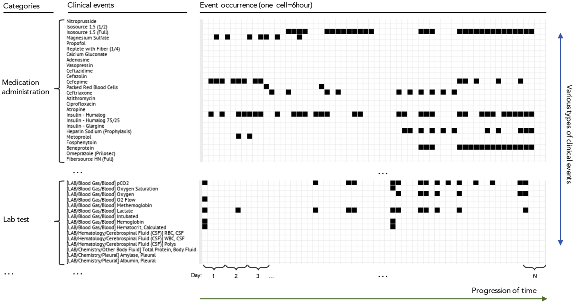
A part of a patient’s record in real-world EHRs (MIMIC-III database) that represented as a sparse matrix. Rows correspond to different clinical events and columns correspond to time. Each cell (bin) indicates occurrence or non-occurrence of an event during a time-window (e.g., 6 hours).

One challenge of using EHR-derived multivariate clinical event time-series is their complexity. For example, tens of thousands of clinical events could occur, but some events occur rarely. Due to its high-dimensional and sparse nature, EHRs data incur challenges for many machine learning algorithms. In the case of MIMIC-III database¹ [5], more than 30,000 different types of clinical events exist, but the average number of occurrences² of each event across event category is usually small. More specifically, average number of medication administrations is 10.1, lab tests 7.3, and procedures 1.5. Furthermore, EHR-derived sequential data consists of heterogeneous events. Each event has different characteristics and complex dependencies to the same or different events that occurred before it. Also, in EHR-derived sequential data, many events co-occur, and this contributes to the complexity in modeling and predicting EHR-derived sequential data. To fully utilize EHRs data, it is important to resolve these issues. Hence, in this work, we focus on developing efficient and scalable methodologies to address these challenges.

1.1. Clinical Event Time-series and Prediction

Briefly, event time-series is a time-series of events that occur in continuous time. In statistics, these are modeled as temporal point processes, that is, point processes defined on time dimension [6, 7, 8]. The basic temporal point process defines occurrence of just one type of event. Marked point processes associate values with each event [9, 10]. If values associated with events are categorical, they represent multivariate event processes. That is, each event category defines its own basic point process [11]. In the context of EHR-derived sequential data, multivariate clinical event time-series is a representation of patient records projected to multiple event time-series where each event time-series represents a specific type of clinical event, such as administration of medication.

The task of predicting multivariate event time-series is defined as follows: given a full history of events in a sequence y_[1:t] (from the beginning until current time t) predict the occurrence of the next (future) event. For continuous-time prediction, this is typically done by defining and modeling an intensity function of the point process. Hawkes process models [12, 13] or its variants [11, 14] can be used for this case. However, instead of defining and learning the intensity function for continuous-time prediction, one may also restrict predictions to a finite time interval (window). As the event time-series is multivariate, $y_{i=1}^t$ can be represented by a multi-dimensional binary vector, as shown in Figure 3. Detailed introduction of the multivariate event time-series and formal definition of the prediction task will be shown in Section 2.

Figure 3:

Prediction task defined over the multivariate clinical event time-series introduced in Figure 2. Given the full patient event history (blue box), the goal is to predict occurrences of each event in the future window (purple box).

1.2. Clinical Relevance of the Event Prediction Models

Our work develops predictive models for a broad range of events in EHRs. These models can be used for different purposes. If events predicted are equal to adverse events our ability to predict boils down to adverse event predictions. Examples of such problems are predictions of sepsis [15, 16] or acute kidney injury [17]. However, we would like to note that some adverse events may not be directly logged in the EHR. In that case, surrogate events and conditions can be used to define these events and enrich the EHR data with augmented event sets. For example, one may define the sepsis event by the time when the standardized Sepsis-3 definition is satisfied [18]. Similarly, AKI prediction targets can be incorporated into EHR using AKI definitions based on the serum creatinine levels and urine output [19, 20, 21].

Our event prediction models can be also used for outlier detection and medical error detection as defined in the works of Hauskrecht et al. [22, 23, 24, 25]. Briefly, by defining high-quality models for predicting the events like lab orders or medication administration, one can use them to infer unexpected omission or commission of medications or labs. Finally, our ability to predict the occurrence of future events for multiple patients at the same time can be used to predict various future resource demands which in turn can be used to optimize the workflows or predict various capacity limits.

1.3. Existing Approaches to Clinical Event Time-Series Prediction

In what follows, we briefly introduce existing approaches to predicting and modeling EHR-derived multivariate event time-series.

• Temporal Templates. Early work on predicting clinical events from EHR data had focused on patient state models generated by predefined temporal templates (featurization) of individual time series and their combinations [23, 26]. Briefly, the temporal template approach transforms complex multivariate clinical time-series with either discrete and realvalues into fixed-sized vector representations. The key idea of the method is to define a set of feature functions (also called feature templates) that map time-series defined over clinical variables to fixed-size vectors and their combinations [23]. The advantage of the methods is that it allows efficient processing of complex EHR-based sequence data into feature vectors that feed (off-the-shelf) classification algorithms such as support vector machines (SVM), Naive Bayes classifiers, decision trees, or neural networks for future event prediction. The approach has been successfully used for different EHR prediction [27, 28] and outlier detection [24, 25] problems. The main disadvantage of the approach is that temporal templates should be defined a priori and the number of possible features generated with these methods can be very large. One solution to alleviate the need to define the templates apriori is to use predictive patterns extracted directly from data using frequent data mining methodologies [29, 30, 31]. Frequent data mining methodologies have been used to modeling complex clinical temporal processes such as onset of adverse events following immunizations [32], drug-drug interactions [33], treatment of acute coronary syndrome [34], patient management of diabetes mellitus [35, 36] and other chronic diseases [37].

  Finally, Sheetrit et al. [38] have developed temporal probabilistic profiles (TPF) for sepsis onset prediction that model frequently repeating temporal patterns of multivariate ICU time-series. However, unlike our approach that predicts a wide range of events, the objective of TPF is to predict the future occurrence of a single target event from multivariate input time-series.

• Probabilistic Latent State Models. More recent work has focused on defining the patient state and predictions using various probabilistic latent state-space models such as hidden Markov models, linear dynamical systems [39, 40], Gaussian processes [41, 42] or their combinations [43]. The approach allows more flexibility by modeling complex dynamics of the clinical time-series through a (shared) latent state-space which is defined by an autoregressive function of a previous latent state and a recent observation. The benefit is that correlated observations can be represented more compactly in the latent space. A limitation of probabilistic models is that the behavior and expressiveness of the latent state-space are determined by a specific (pre-defined) probabilistic distribution such as Gaussian distribution, Bernoulli distribution, or Weibull distribution which may not exactly fit the observed data.

• Modern Neural-based Models. In most recent years, the advances in modern latent embedding and deep learning models led to new low-dimensional latent state representations with good predictive performances on a variety of tasks. Examples of the relevant works include modeling of patient state using real-valued vector-based representation methods such as Skipgram and CBOW [44, 45, 46, 47, 48], or hidden state-space models based on recurrent neural networks (RNN) [49, 50, 51, 52, 53, 54, 55, 56, 57]. These modern approaches typically do not assume specific probabilistic distribution form for generating the hidden state space. Instead, they use a data-driven approach to learn a mapping of the input to the hidden state and ultimately to the output using a series of linear transformations (matrix multiplications) and non-linear activation functions (e.g., sigmoid or tangent hyperbolic). Hence, it is typically more flexible (no specific distribution form is assumed) compared to the probabilistic latent-space approaches.

In this work, we build upon and explore models based on modern neural-based temporal methods.

1.4. Challenges and Directions

Modeling of EHR-derived multivariate clinical event time-series is not an easy task and it comes with a number of challenges which we review below.

1.4.1. High Dimensionality

Multivariate clinical event time series for hospitalized patients consist of several thousands of different types of clinical events corresponding to the administration of many different medications, lab orders, lab results, various physiological observations, procedures, etc. For example, as mentioned before, there are more than 30,000 different types of events exist in MIMIC-III Database. When representing multivariate event time-series in a matrix form, such as in Figure 2, the matrix becomes large and sparse, and its complexity may not fit well standard statistical time series models [58].

To address this issue some works attempted to predict a singly occurring target event (i.e., one type of target event) instead of concurrently predicting all multivariate events [46, 49, 51, 52, 53, 59]. In this work, we aim to predict high-dimensional targets from the sequence of high-dimensional events. It is more challenging as the models need to learn more complex associations between context and target over multiple time steps.

1.4.2. Time-Representation and Temporal Granularity

The original EHR-based multivariate event time-series consist of events recorded in continuous time. To efficiently process the time-series, the original continuous-time representation is typically transformed into discrete-time based representation using window-based segmentation [24, 25, 54, 57, 60] which maps multiple events that happen during a specific time-window in a fixed-sized binary vector. During the segmentation process, the derived event time-series can be generated at a certain temporal granularity that corresponds to the window’s size. Finer temporal granularity results in a more detailed (high-resolution) representation of patient states that leads to longer and sparser sequences which in turn make the modeling of event dependencies much harder, and computationally more expensive.

To alleviate these problems, some of the prior works on modeling HER-based event time-series used coarser temporal granularity such as admission or visit level [46, 50, 52]. In this work, we consider and build models with event time-series based on finer temporal granularity with a segmentation window (a time-step in a sequence) corresponding to 24, 12, or 6 hours intervals.

1.4.3. Different Temporal Characteristics

The EHR-based multivariate event time-series consists of individual event time-series that have different temporal characteristics. For example, some types of events occur repetitively with certain time gaps (e.g., medications administered at regularly scheduled intervals, as shown in Figure 4). Also, each event has different temporal ranges of dependencies for precursor events. Some events are strongly dependent on very recent occurrences of other events. For example, the administration of norepinephrine (a medication that increases blood pressure) is highly related to an observation of hypotension (low blood pressure state) in its recent past. In other instances, events may depend on a preceding event that occurred a long time ago. For example, the incidence of acute kidney injury (AKI) in the distant past can impact the necessity of dialysis. To accurately predict future events from the multiple event time-series with different temporal characteristics, we need more flexible and expressive models. In this work, we focus on developing methods that can model different temporal characteristics with its modularized architecture. Specifically, we develop models that consist of a set of modules where each focuses on a specific temporal attribute. With this approach, we can build an expressive and flexible ensemble model for multivariate time-series prediction.

Figure 4:

Histogram of time differences for two consecutive events of administration of fluconazole, antibiotics medication. It illustrates how events in EHRs occur with periodicity.

1.5. Overview of Our Approach

To alleviate the outlined challenges, we propose a new autoregressive neural temporal model that can handle complex multivariate event time-series with more expressiveness by equipping different information channels for various temporal characteristics of the event time-series. We particularly hypothesize that events in EHR-based multivariate event time-series has dependencies with certain temporal structure and proper handling of various temporal dependency structures could enhance the predictability of a future event. Specifically, we focus on the following temporal structures of the EHR-based event time-series: The patient information from longer-term distant past is abstracted through hidden states of the neural abstraction module that is based on Long Shortterm Memory (LSTM) [61]. The recent information on the patient state is compiled by recent context module that projects the recent event information into discriminative space. The patient information from repeatedly occurring events is modeled through periodicity mechanism that compiles each event’s periodic statistics into external memory and utilizes in prediction of next event occurrence based on the elapsed times of recent past occurrences. With the three modules, our model can summarize and utilize different aspects of complex clinical event time-series toward accurate prediction of future event occurrence.

To evaluate our model, we use the real-world clinical data derived from EHRs of critical care patients in MIMIC-III database [5]. The clinical events considered in this work correspond to multiple types of events, such as medication administration events, lab test result events, physiological result events, and procedure events. These are combined in a dynamically changing environment typical of intensive care units (ICUs) with patients suffering from severe life-threatening conditions. Through rigorous evaluations on MIMIC-III data we show that our model outperforms multiple baseline models in terms of the quality of event predictions. To provide further insights into its benefit and prediction performance, we also split the results with respect to different types of clinical events considered (medication, lab, procedure, and physiological events), as well as, based on their recurrence patterns, again showing the superior performance of our model.

2. Background

In this section, we first define the multivariate event time-series, their representation, and the prediction task considered in this work. After that, we review work and approaches for multivariate time-series modeling and their applications to clinical event time-series.

2.1. Multivariate Event Time-Series

We define multivariate event time-series by a time-stamped sequence of events U = {u_j}_j, where each event u_j = [e_j, t_j] is represented by a pair of an event type e_j and its time t_j. We assume there are |E| different event types defining the multivariate event time-series. A univariate event time series would be defined by a single event type |E|=1.

The event time series (with continuous time stamps) can be directly modeled using point processes [6, 7, 8]. Examples of such processes are a Poisson process [62] or a Hawkes process [12, 13] and its variants [11, 14]. These models have been applied to various event sequence problems, including clinical event prediction [11, 14]. However, these models are known to be hard to optimize directly using gradient-based methods and require additional sampling methods to compute the integral of log-likelihood of intensity function. Intensity functions defining the point process are functions of time and are very challenging to model and optimize, especially in multivariate settings with many possible dependencies among the different events. Hence, the event time series are often converted to discrete-time models (see Figure 5) where the original event time series are segmented using a window spanning a certain fixed period of time, and events within the window are considered to co-occur in the discretized time.

2.2. Segmentation (discretization) of Event-Time Series

We define the discrete-time event time-series as follows:

• Discrete-time event time-series Y = {y_i}_i consist of a sequence of states y_i where y_i ∈ {0, 1}^|E| is a multivariate binary vector that represents occurrences of events of different types at a discrete time step i, and |E| denotes the total number of event types.

• Discrete-time event time-series are generated from time-stamped multivariate event time-series U through segmentation of event occurrences with a time window W as described in Figure 5.

In the following sections we assume we have data that consists of N discrete-time event time-series: D = {Y₁, …, Y_N}. Next, we review existing modeling approaches for the discrete-time event time-series.

2.3. Markov Models

Markov models form a foundation of discrete-time time-series models. Given their simplicity and tractability, the majority of the event time-series models are special cases of Markov models [63, 64]. Markov models represent a sequence of observations over time using a sequence of states and their transitions. The Markov property assumes that the current state captures all necessary information relating the future and past. In other words, the next state depends only on the most recent state, and is independent of the past states:

$$P\left(y_T|y_{T-1},y_{T-2},\dots ,y_1\right)=P\left(y_T|y_{T-1}\right)$$ (1)

The joint distribution of an observed sequence is modeled by a product of conditional probabilities:

$$P\left(y_1,y_2,\dots ,y_T\right)=p\left(y_1\right)\prod _{i=2}^{T}P\left(y_i|y_{i-1}\right)$$ (2)

A standard Markov model assumes all states of the time series are directly observed. However, the states of many real-world processes are not directly observable. One way to resolve the problem is to define the state in terms of a limited number of past observations or features defined on past observations [25, 26, 65] and another is to use Markov models with hidden states.

2.3.1. Hidden Markov Models

A Hidden Markov model (HMM) [66, 67] introduces hidden states z_i of d×1 dimension. The observation y_i is modeled through the hidden state z_i and the emission table $B\in {ℝ}^{|E|\times d}$ with components: B_m,n = P(y_i = n|z_i = m). The transition table A is used to update the hidden states and the emission table B is used to generate observations:

$$z_i=A\cdot z_{i-1}\hspace{1em}\hspace{1em}\hspace{1em}{y}_i=B\cdot z_i$$

The prediction for next event y_i+1 can be made straightforwardly, given the hidden state of the current time step z_i: P(y_i+1|z_i) = B · (A · z_i).

Clinical Applications.

HMMs have been shown to reach good performance in many applications such as stock price prediction [68], DNA sequence analysis [69], and time-series clustering [70]. For clinical tasks, HMMs have been used to model dynamics of various clinical variables such as progressions of glaucoma and Alzheimer’s disease [71], epileptic seizure events [72], medication administration patterns from post-surgical cardiac patient [73], and neonatal sepsis events [74].

Traditional HMM models assume discrete (categorical) hidden states. Linear dynamical systems (LDS) [75, 76] alleviate this issue by defining real-value hidden and observable states. Another issue with the hidden state in Markov models is that the dimensionality of their hidden state space is not known a priori. Various methods for hidden state space regularization, such as [39, 40, 77] have been able to address this problem.

2.4. Neural-based models for event time-series

Recent advances in neural architectures and their application to time-series offer end-to-end learning framework that is often more flexible than standard time-series models. In this section, we summarize the following neural-based methods for event time-series processing: recurrent neural network (RNN), long short-term memory (LSTM), attention mechanism, and convolutional neural network (CNN).

2.4.1. Recurrent Neural Network

RNN is a type of neural network that models a sequence with the hidden state, similarly to HMM. But RNN is more flexible and efficient: given fixed input and target from data, RNN is to learn the intermediate association between them. Unlike HMM, the value of the hidden state of RNN is computed purely deterministically. Without any stochastic component, at each time step t, the hidden state h_t is computed given the previous time step’s hidden states h_t−1 and new information from the current time step’s input y_t with the following rule:

$$h_t=\text{tanh}\left(U\cdot y_t+W\cdot h_{t-1}\right)$$

where tanh(·) is hyperbolic tangent used as an activation function that helps it to learn non-linearities. $U\in {ℝ}^{d\times |E|}$ and $W\in {ℝ}^{d\times d}$ are weight matrices. Once trained, the same weights are shared over time. Hence, no smoothing or filtering is required to compute the values of the hidden state. The prediction for the next event ${\widehat{y}}_{t+1}$ is generated as follows:

$${\widehat{y}}_{t+1}=g\left(V\cdot h_t\right)$$ (3)

where $V\in {ℝ}^{d\times |E|}$ is output layer weight matrix and g(·) is an output transformation function. g(·) can be any activation function, and it needs to be selected to match the type of the target in data. For instance, if the target variable is a multi-class variable the softmax function is used. On the other hand, if the target is binary or is defined by a set of binary variables a sigmoid function (such as logistic function) is used. The parameters of RNN are learned through a stochastic gradient descent algorithm. Loss is determined by cross-entropy function (multi-class) or binary cross-entropy function (multi-label), summed over all time-steps of each sequence as well as across all sequences [78].

Meanwhile, RNN is known to have limitations on learning and prediction with long sequences, problems are called vanishing and exploding gradient [79]. Several solutions are proposed for the problem. One is to apply backpropagation on chunked sequence with a limited number of time steps (Truncated-BPTT) [80, 81]. Another is to add gates to produce paths where gradients can flow more constantly in longer-term without vanishing or exploding such as Long Short-Term Memory (LSTM) [61] and Gated Recurrent Units (GRU) [82].

2.4.2. Long Short-Term Memory

LSTM effectively prevents the vanishing and exploding gradient problems with memory cell states and gates that control the information flow. Each gate is composed of linear transformation with sigmoid activation function on h_t−1 and y_t. In detail, the hidden states h_t and cell states C_t are updated as follows: first, LSTM updates the candidate for the new cell states ${\tilde{C}}_t$ as a function of h_t−₁ and y_t:

$${\tilde{C}}_t=\text{tanh}\left(W_c\cdot \left[h_{t-1},y_t\right]+b_c\right)$$ (4)

where [, ] represent concatenation of two vectors. Then, it computes forget f_t and input i_t gates which will be used to determine how much contents from the previous cell C_t−1 will be erased and how much of values of the new candidate cell states ${\tilde{C}}_t$ combined into the new cell state C_t respectively:

$$\begin{gathered} f_t=\sigma \left(W_f\cdot \left[h_{t-1},y_t\right]+b_f\right) \\ {i}_t=\sigma \left(W_i\cdot \left[h_{t-1},y_t\right]+b_i\right) \\ {C}_t=f_t\cdot C_{t-1}+i_t\cdot {\tilde{C}}_t \end{gathered}$$ (5)

Output hidden states h_t will be based on the cell state C_t with filter from output gate o_t which decides which part of the cell state C_t will be in the output:

$$o_t=\sigma \left(W_o\cdot \left[h_{t-1},y_t\right]+b_o\right)h_t=o_t\otimes \text{tanh}\left(C_t\right)$$ (6)

where ⊗ denotes element-wise multiplication and W_f, W_i, $W_o\in {ℝ}^{|E|\times d}$ and $W_c\in {ℝ}^{d+|E|\times d}$. With these parameters ready, we can simply denote LSTM as a function of the previous hidden states h_t−1 and current time-step’s input y_t:

$$h_t=\text{LSTM}\left(y_t,h_{t-1}\right)$$

The final prediction for the next event ${\widehat{y}}_{t+1}$ is computed the same way as RNN in Eq. 3. The parameters are also trained through the same method used for RNN.

Clinical Applications.

RNN and LSTM have been applied to many areas of prediction and modeling of sequence data such as time series [83, 84], vision [85], speech [86], and language [87] problems and many others. For modeling of clinical event time-series, the hidden states of RNN and LSTM can directly correspond to a real-valued (latent) representation of patient states. With this property, RNN and LSTM have been successfully applied to many clinical event predictions such as medication prescriptions [50, 88], heart failure onset [89], readmission of chronic diseases [90], outcome of kidney transplantation [52], disease progression of diabetes and mental health [53], and ICU mortality risk [55]. Specifically, Bajor et al. [88] tested performances of LSTM and GRU [82] models along with non-recurrent models such as random forests [91] on the task of predicting the next medication given a sequence of ICD-9 diagnosis codes. Also, Choi et al. (2017a) [89] tested GRU with non-sequential models such as SVM [92] and Multi-Layer Perceptron (MLP) for the task of predicting the onset of heart failure given events such as disease diagnosis, medication orders, and procedure orders that happened within a fixed observation window from longitudinal EHRs data. Choi et al. (2016b) [50] used GRU to predict diagnosis and medication at a next visit given a sequence of diagnosis codes, medication codes, or procedure codes in previous visits. Esteban et al. [52] used RNN to predict the outcomes of kidney transplant operations given a sequence of medications, lab tests along with and demographic and static information about patients such as age, gender, blood type, weight, primary disease. One challenge of modeling EHR-derived time-series is that data are sparse, and values for many clinical variables are missing. An example of a probabilistic model that deals with these problems for real-valued clinical variables is the work of Liu et al. [93]. An example of an RNN-based approach for the same problem is the work of Che et al. [94]. It augments GRU with a novel mechanism called GRU-D that decays hidden states and inputs to capture the missing temporal patterns explicitly. However, we note that our work aims to predict discrete event occurrences while the GRU-D is designed to model real-valued time-series; hence it is not applicable to event time series.

2.4.3. Attention Mechanism

When the length of a sequence is longer, it typically deters RNN/LSTM to learn dependencies between distant positions [79, 95]. Attention mechanism [96] tackles the challenge by using hidden states of all available time steps h₁, …, h_t, instead of the last one h_t. At current time step t, attention mechanism generates an output o_t as a weighted sum of h₁, …, h_t. Softmax is used to compute the attention weight ${\alpha }_i^t$ which measures relative importance of h_i among all available hidden states h₁, …, h_t to the output o_t. The weight is computed through as follows:

$${\alpha }_i^t=\frac{\text{exp}\left(\text{score}\left(h_i,q_t\right)\right)}{{\sum }_{j=1}^t\text{exp}\left(\text{score}\left(h_k,q_t\right)\right)}$$ (7)

Typically, the previous time-step’s output o_t−1 is used for the query term q_t. In the original paper [96], the score function is parameterized by a simple feed-forward neural network with tangent hyperbolic (tanh) activation:

$$\text{score}\left(h_i,q_t\right)=v_a\cdot \text{tanh}\left(W_a\cdot \left[h_i,q_t\right]\right)$$ (8)

where v_a and W_a are weight vector and matrix. Then, we can compute the output o_t as a weighted sum of hidden states:

$$o_t=\sum _{i=1}^t{\alpha }_i^t\cdot h_i$$ (9)

For prediction, o_t is plugged into Equation (3) at the place where h_t is used: ${\widehat{y}}_{t+1}=g\left(V\cdot o_t\right)$.

Clinical Applications.

Attention mechanism has been widely adopted in many machine translation and NLP tasks [97, 98, 99, 100, 101, 102]. For the clinical sequence modeling, attention mechanism has been applied to the treatment (medication) recommendation [103], prediction of sequential diagnoses and heart failure prediction [49, 104], and prediction of in-hospital mortality, readmission rate, and length of stay [60], and in these works, attention-based approaches consistently show outperforming results over RNN/LSTM based models. Specifically, Zhang et al. [103] developed a model that learns a predictive mapping between a bag of diagnoses at a visit (input) and a bag of medications at the same visit (labels). The relationship between medications is modeled through attention mechanism, and the relationship between medications and diseases is modeled through an RNN-based decoder, which sequentially predicts the most probable medication at each time-step. Choi et al. (2016a) [49] approached next diagnosis prediction task (multi-class sequential prediction) and heart disease onset prediction (binary sequence classification) with reverse-time attention mechanism (RETAIN). Briefly, it computes hidden states of RNN in reverse time-order and uses two attention mechanisms to compute attention weights. Interestingly, Choi et al. (2017b) [104] used attention mechanism to comprehend prior knowledge in medical ontology for sequence prediction. In detail, the authors developed a sequential diagnosis prediction model that predicts all diagnosis categories in the next visit. The model uses the attention mechanism over a tree-like structured knowledge graph (ICD-9 diagnoses code ontology) to compose a representation of a leaf diagnosis code as a weighted average of ancestor nodes. Leveraging prior knowledge in ontology led to better predictability compared to GRU-based baseline models.

2.4.4. Convolutional Neural Network (CNN)

Unlike RNN/LSTM that recurrently computes an internal representation of sequences over time, Convolutional Neural Network (CNN) [105] uses a different mechanism to summarizes the history of past events: briefly, it first uses sliding (convolving) filters over time to compute local features. Then, after processing the local features into non-linear activation function (e.g., ReLU), it uses pooling operation to summarize the local features. Particularly, CNN is known to be powerful in dealing with complex input features (such as ones in images and videos) due to its key properties: location invariance and compositionality. Location invariance: from high dimensional input, convolution and pooling operations help to extract key information regardless of the location of the key information. That is, CNN is invariance to scaling to extract key features. Compositionality: each convolutional filter creates a local patch (information channel) of lower-level features into a high-level representation. Typically, multiple convolutional filters of different sizes are used together, and this creates multiple channels that effectively summarize local features with different scales and projections. Especially, with a deeply layered network structure, important information for a task (e.g., classification) is hierarchically composed from bottom to top.

Clinical Applications.

CNN has been very successfully used in wide areas including image recognition [106, 107, 108, 109], object detection [110, 111, 112], text detection and recognition from images [113, 114, 115], automatic speech recognition [116, 117, 118]. Also, CNN also has been used to NLP tasks such as text classification [119, 120, 121] and language modeling[122, 123, 124]. For clinical time-series such as complex high-dimensional real-valued biomarkers (e.g., lab values) or discrete event sequences, CNN has been used to predict clinical events [125, 126, 127] (e.g., the onset of disease) and clinical outcomes [59]. Specifically, Razavian et al. [125] leveraged CNN to predict the onset of diseases (ICD9 code) given time-series of lab test values of patients. Suresh et al. [126] tested CNN and LSTM for the prediction of five intervention tasks given numeric lab values and clinical free-text notes over time: invasive ventilation, non-invasive ventilation, vasopressors, colloid boluses, and crystalloid boluses. To obtain feature representation of complex clinical free-text data, they used a topic distribution of the notes learned from Latent Dirichlet Allocation (topic modeling) [128]. Nguyen et al. [59] used CNN to predict readmission rate given previous clinical event history (diagnosis and medication). They considered the time-gap between consecutive events as a special token. Cheng et al. [127] used CNN to summarize diagnosis codes (ICD9) of patients for prediction of the onset of congestive heart failure (CHF) and chronic obstructive pulmonary disease (COPD).

2.5. Modeling Periodic Signals

Clinical event time series often come with temporal patterns defined by periodic events. In terms of modeling periodic signals, existing researches have traditionally focused on standard models defined by spectral decomposition of the signals using Fast Fourier Transformation (FFT) [129, 130, 131, 132, 133, 134]. However, FFT is known to require sequential data with comparably high sampling rates [135] and due to this reason, FFT-based approaches may not fit with the modeling of clinical event time-series data which consists of many sparsely occurring events. Temporal pattern mining has been used to model periodic events in sparse sequence data. Ozden et al. [136] introduced a method that discovers temporal patterns with strict periodicities (uniform inter-event intervals) based on association rule mining approaches [137]. Subsequently, Han et al. [138], Ma and Hellerstein [139], and Cao et al. [140] developed methods that can discover relaxed periodic patterns such as periodicities with a few skips in event occurrences or with non-uniform inter-event intervals between event occurrences. Statistical parametric models are also used to model sparsely occurring temporal events. Based on hidden semi-Markov models, Kapoor et al. [141] attempted to model repetitive music listening events. Trouleau et al. [142] model video binge-watching behavior based on a Poisson mixture model with latent factors. Kurashima et al. [143] predicted everyday human actions from smart wearable devices with temporal point processes defined based on Weibull distributions. Using the histogram of inter-visit timing intervals for websites, Adar et al. [144] clustered re-visitations of a website.

3. Methodology

In this section, we introduce a new autoregressive event time-series model that represents different aspects of multivariate clinical event-time series with multiple temporal mechanisms. Briefly, information from the distant past is abstracted and carried through the hidden states of the LSTM-based neural abstraction module. Information about the most recent observations (context) is processed by the recent context module. Finally, information about event recurrence and their periodicity is modeled and processed through a periodicity-aware mechanism. The final event prediction model combines all three channels of information and outputs the probabilities of multivariate event occurrences for the next time step. The architecture of the proposed model is summarized in Figure 6. In the following, we describe each module and its role in depth.

Figure 6:

Architecture of the proposed model. Different temporal aspects of information in the multivariate event time-series (y₁, …, y_t−1, y_t) are processed through three different mechanisms: neural abstraction, recent context and periodicity memory modules.

3.1. Neural Abstraction Module

LSTM has been successfully used to model time series with the help of hidden states, allowing one to abstract and summarize information from a more distant past. At a glance, at each step of a sequence, LSTM gets (event) input and updates its hidden state based on the hidden state from the previous step. Then it feds predictive signals for the occurrence of events in the next step.

In detail, at each time step t, events in the input sequence represented as binary vector y_t ∈ (0, 1)^|E| are processed and mapped to a real-valued vector z_t through embedding matrix W_emb: z_t = W_(emb) · y_t. Then, given the processed input z_t and previous hidden states h_t−1, LSTM updates hidden states h_t through the update rules defined in Equations 4–6:

$$h_t=\text{LSTM}\left(z_t,h_{t-1}\right)$$ (10)

3.2. Recent Context Module

When properly trained, the hidden state in the LSTM module can be sufficient to represent and model future behaviors of event time-series by abstracting dependencies of past and future events. However, to be trained properly, LSTM (or any deep-learning based models) requires large amounts of training instances. In the clinical domain, obtaining large amounts of clinical cases (e.g., rarely ordered medication or lab tests) is hard in general. This constraint may deter us from training LSTM for predicting rare clinical cases. Meanwhile, for certain clinical event categories such as medications, an event’s future occurrence may highly depend only on the most recent events and not the distant past. Hence incorporating this information through the hidden state of LSTM does not make much sense. To address the above issues, we propose to distinguish and model two sources of information from past event sequence: (1) the abstracted information of past event sequence through hidden states of LSTM representing more distant past and (2) the specific information about event occurrences in a very recent context window. The recent context module serves to capture and process the recent event information. Briefly, the recent event at the current time step t is in binary vector y_t ∈ (0, 1)^|E| and it is incorporated into the model through a linear transformation to model:

$$b_u=W_s\cdot y_t+b_s$$ (11)

b_s can be seen as additional bias term that reflects recent event occurrence information.

3.3. Periodicity Memory Module

Many events in the EHR-based multivariate event time-series occur periodically. For example, administrations of various medications occur with certain periodicity due to the nature of the medication administration dosage regime. Figure 9 shows the distribution of time gaps between two consecutive administration events for one of the medication with a typical period of 12 hours.

Figure 9:

Histograms of inter-event gaps of two consecutive occurrences of the top performing events shown in Figure 2

One approach to modeling the periodicity of the time-series is to rely on the hidden states of RNN/LSTM. Briefly, if the RNN is properly trained, it could figure out sufficient statistics and counting processes needed to drive periodic signals. However, when the number of the different periodic events in the EHR is large, it is not feasible to expect the model will be able to cover all periodic events using the same hidden state (of limited size). To prevent this from happening, we propose a simple mechanism to enhance the handling of periodic events and incorporate them into the periodicity module. Briefly, the new module relies on a memory that stores observed temporal characteristics of many periodic events and uses them to derive a new periodicity-aware signal to enhance event predictions further, and this at any time and for any prediction window size.

In a nutshell, our module uses memory that stores gaps (time differences) observed for pairs of two consecutive events of the same type (a) for all past patients and (b) for the current patient. At the time of the prediction for the current event time-series, the module calculates how much time has elapsed since the latest occurrence of the event of the same type, and based on the prediction window size and information stored in the memory of past event gaps, it predicts the probability of the signal to be repeated in the next prediction window. As noted earlier, two different sources of information are used: (a) event gaps for the current patient and (b) compiled event gap distributions obtained from time-series of past patients in the training set. We describe the event prediction mechanisms in more detail in the next subsections.

3.3.1. Event Prediction Based on Recent Event Gap for the Current Patient

The periodicity module models periodicity of individual patient’s event stream and utilizes it for predicting the next occurrence of each event type. To predict the future occurrence of event e ∈ E for the current patients, we use two periodicity-related statistics:

• Recent interval (ζ), that is a time period between the two most recent occurrences of the event e in the current event stream:

  $${\zeta }_t^e={\tau }_t^e-{\tau }_{t-1}^e$$

  where ${\tau }_t^e$ and ${\tau }_{t-1}^e$ are timings of the two most recent occurrences of the event e in the current event stream (that is, events closest to current time t).
• Elapsed time (ϵ) that is the time elapsed from the last occurrence of the event e in the current stream:

  $${ϵ}_t^e=t-{\tau }_t^e$$

  where t denotes the current time.

With the above two statistics, the model outputs patient-specific periodicity-based prediction $p_t^e$ for event e and the prediction window of size W: as

$$p_t^e=\{\begin{array}{ll}1\hfill & \text{if }{ϵ}_t^e<{\zeta }_t^e<{ϵ}_t^e+W\hfill \\ 0\hfill & \text{otherwise}.\hfill \end{array}$$ (12)

One drawback of this approach is that it cannot make predictions until it observes the first two occurrences of events (τ₁ and τ₂). In addition, the recent interval statistic keeps only recently observed time gap between the two consecutive events for the current patient and hence its predictions may become inaccurate. To address this issue, we rely on event gap statistics and their distribution as obtained from the training patient set.

3.3.2. Event Prediction Based on Event Gap Distribution of Past Patients

The probability distribution of event gaps (time differences between two consecutive events) for each individual event type can be compiled from across all patients in the training set and represented (non-parametrically) in a histogram structure. Figure 7 illustrates such a histogram.

Figure 7:

Event gap distribution and calculation of the probability of future event occurrence. Event gap distribution is formed by summarizing event gaps observed in time series of past patients and compiling them into a (normalized counts) histogram. The event prediction for the current time t and prediction window W is made by calculating the histogram probability mass defined by the time elapsed since the last event and the size of the future prediction window (sum of probabilities inside yellow solid line) and by normalizing it with the remaining probability mass defined by current time and onward time (sum of probabilities inside green dotted line).

To predict the probability of occurrence of the next event e in the prediction window W for the current patient’s time-series, the histogram structure, the time elapsed since the most recently observed event ${ϵ}_t^e$, and size of the prediction window W are considered. To do so, we define a function mass(t_a, t_b) that returns the probability mass between two time points [t_a, t_b] (such that t_a < t_b) when projected on the histogram. Then, the signal $r_t^e$ predicting the probability of the next event occurrence within the next time window based on the histogram probabilities is defined as follows:

$$r_t^e=\frac{\mathit{\text{mass}}\left({ϵ}_t^e,{ϵ}_t^e+W\right)}{\mathit{\text{mass}}\left({ϵ}_t^e,\infty \right)}$$ (13)

This process is illustrated in Figure 7. Briefly, the numerator reflects a probability of observing the next event from the current time (projected on the event gap histogram using the elapsed time since the most recent event time) to the new time defined by the window size W. The denominator defines a normalizer that takes into account the fact that no event has been seen during the time period defined by the elapsed time and basically corresponds to the probability of observing the event from the current time till the infinity. We assume that $r_t^e=0$ if there is no prior occurrence of the event e.

3.4. Combining Predictive Signals

With the predictive signals b_u (Eq. 11), h_t (Eq. 10), $p_t^e$ (Eq. 12), and $r_t^e$ (Eq. 13) ready, we compute final output of the model as follows: First, we compute event-specific intermediate output ${\tilde{o}}^e$:

$${\tilde{o}}^e=\left(W_{\mathit{\text{out}}}^e\cdot \left[h_t,p_t^e,r_t^e\right]+b_{\mathit{\text{out}}}^e\right)$$

where $W_{\mathit{\text{out}}}^e\in {ℝ}^{1\times (h+2)}$ and $b_{\mathit{\text{out}}}^e\in ℝ$ are parameters of the linear transformation of the vector combining all signals. The final output for next event occurrence is computed as follows:

$${\widehat{y}}_{t+1}=\sigma \left(\left[{\tilde{o}}^1,\dots ,{\tilde{o}}^{|E|}\right]+b_u\right)$$ (14)

The proposed predictor combines information on distant past from LSTM’s hidden states and event gap-based information from the periodicity module through concatenation and important signal for each event e is selected through linear regression parameterized with $W_{\mathit{\text{out}}}^e$, $b_{\mathit{\text{out}}}^e$. Then, the recent state (most recent events) information is added as an additional recent bias term. The addition of the recent bias can be seen as adjusting information from LSTM’s hidden states and the periodicity module with information from recent event occurrences.

3.5. Parameter Learning

The parameters of the model are learned by backpropagation through time (BPTT) [145] with an adaptive stochastic gradient descent based optimizer (ADAM) [146]. For loss function $\mathcal{L}$, we use binary cross entropy between the prediction vector ${\widehat{y}}_t$ and the true event occurrence vector y_t over all sequences in the training set and 1 denotes a vector filled with 1s:

$$\mathcal{L}=\sum _t-\left[y_t\cdot \text{log\hspace{0.17em}}{\widehat{y}}_t+\left(1-y_t\right)\cdot \text{log}\left(1-{\widehat{y}}_t\right)\right]$$

For the prior event gap distribution, the parameter are learned nonparametrically by counting and normalizing the histogram bins of each event-type.

4. Experimental Evaluation

In this section, we evaluate the performance of our new autoregressive model on MIMIC III data [5] and compare it with alternative baselines.

4.1. Clinical data

We test the proposed model on MIMIC-III, a clinical database generated from real-world EHRs of intensive care unit patients [5]. We extract 5137 patients from the database by applying the following selection criteria: (1) adult patients with age between 19–99 (2) patients with a length of ICU stay between 48 and 480 hours, and (3) patients with records represented in the Meta Vision, one of the systems used to generate MIMIC-III dataset. Except for these criteria, we do not filter out any patient in order to test our model across the general patient pool regardless of disease, symptoms, or conditions. We split the patients into the training and test sets with a ratio of 8:2.

For the sake of the robust experimental evaluation, we build ten different train-test data splits by randomly shuffling the patients before splitting. We report averages over these ten different splits.

4.1.1. Feature Preparation

We generate discrete-time event time-series by segmenting all EHR sequences with three different window sizes (W=6,12,24 hours). As mentioned in Section 2.1, at each step of a window segment, the input y_t is as a binary vector formed by aggregating all types of events in the window and the prediction target y_t+1 is formed as a binary vector of events that occurred in the next window segment. We use four clinical event categories: medication administration events, lab results events, procedure events, and physiological result events. For medication, lab, and procedure event categories, we filter out those events observed in less than 500 different patients. Further, for each of 10 splits, we filter out those events that are not observed in both train and test sets. The number of resulting events (|E|) is 282. The table 1 shows relevant data statistics collected from the train set.

Table 1:

Clinical data statistics by event categories (W=6)

Category	Medication	Procedure	Lab test	Physio signal
Cardinality	64	44	155	19
Num. of occurrences across all patients	59K	53K	308K	181K
Avg. rate of occurrence throughout all time-windows	5.8%	7.6%	12.7%	60.9%
Median number of event occurrences per admission	4	2	4	12
IQR of number of event occurrences per admission	6	12	7	15

4.2. Baseline models

We compare our model with multiple baseline models that can predict events for multivariate event time series given their previous history. The baselines are:

• Logistic Regression based on the Recent Context information (LR-Recent) predicts the next event occurrence y_t+1 using the current events y_t. The model is defined by a linear transformation with the sigmoid output function: ${\widehat{y}}_{t+1}=\sigma \left(W_{lr}\cdot y_t+b_{lr}\right)$, $W_{lr}\in {ℝ}^{|E|\times |E|}$.

• Logistic Regression based on the Full history (LR-Binary): aggregates all event occurrences from the complete past event sequence and represents them as a binary vector. The vector is then projected to the prediction of y_t+1 by using the same parameterization as the above model.

• REverse-Time AttenTioN (RETAIN): RETAIN is a representative of attention-based approaches that uses attention mechanisms to summarize clinical event sequences. Proposed by Choi et al. (2016a) [49], RETAIN uses two attention mechanisms to comprehend the history of hidden states from RNN (GRU) in reverse-time order. For multi-label prediction, we use sigmoid function at the output layer. (See Section 2.4.3 for details of attention mechanism)

• Logistic regression based on Convolutional Neural Network (CNN): This model uses CNN to build predictive features summarizing the event history of patients. Following Nguyen et al. [59], we implement this CNN-based baseline model with a 1-dimensional convolution kernel operation followed by ReLU activation and max-pooling operation. To give more flexibility to the convolution operation, we use multiple kernels with different sizes (2,4,8), and features from these kernels are merged at a fully-connected (FC) layer. (See Section 2.4.4 for details of CNN)

• Logistic regression based on the Hidden States from LSTM (HS): predicts y_t+1 based on the hidden states of the LSTM in Eq. 10. Linear transformation with sigmoid activation function is used similarly to the above models.

• Logistic regression based on the Hidden States from LSTM and Recent Context information (HS-RC): predicts y_t+1 based on hidden states of LSTM and recent context state. The information is projected via linear transformation with the sigmoid activation function at the output.

The proposed model that combines all three sources of information is referred to as HS-RC-PM. (PM stands for Periodicity Memory)

4.3. Evaluation metrics

We evaluate the quality of predictions by calculating the area under the precision-recall curve (AUPRC). AUPRC provides a more accurate performance profile of models for a highly imbalanced dataset [147]. Due to the nature of EHR-derived time-series data, our dataset is highly skewed to negative examples as shown in Table 1.

The reported AUPRC values (for the different methods) are averaged over all target events and over test sets defined by 10 different train/test splits.

4.4. Implementation Detail

For the experiments, we use embedding size 64, fixed learning rate 0.005, and minibatch size 256. The size of LSTM’s hidden states is determined by an internal validation set (a subset of the training set) with ranges of (64, 128, 256, 512), and the tuning results are reported in Figure A.13 in the Appendix. To prevent over-fitting, L₂ weight decay regularization is applied to all models. The amount of weight decay is also learned by an internal validation set for each baseline model.

4.5. Experimental Results

Figure 8 summarizes prediction results for all event types for three window sizes (W=6,12,24) by averaging AUPRC obtained on our model and baselines. We can clearly see that our model, HS-RC-PM, outperforms all baselines with a clear margin in all window segmentation settings. Also, note that AUPRC results for larger window sizes are higher. This is expected since segmentations based on larger window sizes lead to higher priors for the occurrence of the events.

Figure 8:

Overall prediction results. The results show average test AUPRCs over all events and 10 different random train-test splits.

Analyzing the results in Figure 8 by looking at the performance gap between HS-RC-PM and HS-RC, we can see the added benefit of the periodicity module to the prediction performance since the two models differ exactly in the inclusion of that module. Digging deeper to understand this difference, Table 2 shows AUPRCs for some events in which HS-RC-PM brings remarkable enhancement in the predictive performance compared to HS-RC. Figure 9 shows the distribution of event gaps for these events (events in Table 2). Indeed, it is no surprise to observe such a performance improvement given strong periodicity in events. The events with clear periodic behavior translate to the largest performance gap between HS-RC-PM and HS-RC.

Table 2:

Performance on top 9 events with the largest gap between HS-RC and HS-RC-PM (W=6)

Event	HS	HS-RC	HS-RC-PM
[Med] Fluconazole	1.98	2.20	34.54
[Med] Ceftriaxone	5.40	4.79	33.02
[Med] Levofloxacin	3.27	3.27	26.80
[Med] Azithromycin	1.94	2.09	25.04
[Med] Ciprofloxacin	26.97	28.46	50.82
[Med] Metronidazole	52.78	49.43	70.86
[Med] Acyclovir	32.13	31.00	51.63
[Med] Cefazolin	43.69	41.50	60.74
[Med] Cefepime	36.55	35.82	54.38

The benefits of the combination of the hidden state and recent information (HS-RC) over models based on its individual components (HS and LR-Recent) can be observed in smaller window segments W=6, 12 and it is no worse than its component models in larger window segments W=24. When the window size is W=24, the performance of the LR-Recent model approaches and is close to HS-RC. On the other hand, the performance of the LR-Recent on smaller window sizes deteriorates rapidly. This suggests that most of the important information for predicting future clinical events comes from the recent 24 hours. This finding can also be partly explained by the fact that many events (such as drug administrations or lab orders) are repeated every 24-hours, hence once they are observed they are most likely to occur also in the next time window. In terms of pure HS model, the difference from HS-RC model is more visible across all window sizes, but HS contributes to HS-RC predictions visibly more for small window size (W=6), which is in line with the observed reduced benefit of LR-Recent model for that window size.

For the difference between HS and RETAIN, we can observe that RETAIN outperforms HS at W=24 but the inverse occurs at W=6, 12. This can be due to the fact that shorter segmentation windows (W=6, 12) make the input sequences longer and more complex and attention mechanisms in RETAIN may not be able to pick up the important predictive signal from such sequences. On the other hand, with a larger segmentation window (W=24), important predictive information can be condensed into the previous step window, and HS would not have any issues accessing it. Interestingly, we can observe a similar pattern when analyzing the performance of CNN compared to HS. We observe the gap between CNN and HS is larger for a smaller segmentation window. Considering the fact that CNN comprehends whole event history with convolution operations, the longer and more complex sequence is likely to cause CNN to perform worse at sequences from smaller segmentation windows.

4.5.1. Analysis of Results based on Repetition Patterns

The overall results showed the performance boost from the inclusion of the periodicity module. To further verify the effectiveness of the module across all events, we divide the event time-series based on the number of previous events occurrence for each event type and compute the performance for each group. Briefly, we divide the event time-series into three groups: (G1) time-series with no previous event occurrences (from the beginning till the event occurs the first time), (G2) one previous event occurrence (after the event is observed first time till it is observed the second time), and (G3) two and more previous event occurrences (after observing the event the second time and to the end of the time-series). When properly trained, it is expected that the performance gap between HS-RC-PM and HS-RC should be visible for groups G2 and mainly for G3, since the periodicity module is not able to generate any relevant signal until it gets the first event occurrence (case G1). Figure 10 shows the results for these three groups.

Figure 10:

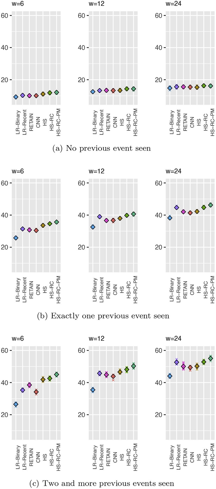
Prediction results based on the number of previous event seen

As expected, the performance gap between HS-RC-PM and HS-RC is widened at G2 as we expected. This clearly reflects the value of the information on periodic events compiled through periodicity memory. Also, differences in the gap between HS-RC-PM and HS-RC in Figure 10b (G2) and Figure 10c (G3) shows how the patient-specific recent interval could be informative toward accurate prediction of the time-series.

4.5.2. Analysis of Results based on Event Categories

To analyze the experimental results further, we next break the evaluation results down by inspecting the predictive performances of the models for the four different event categories: medication events, lab events, physiological events, and procedure events. The results are shown in Figure 11. Clearly, HS-RC-PM consistently outperforms baseline models across all event categories in AUPRC statistics.

Figure 11:

Prediction results by the event type category

Notably, in the medication administration category, the performance gap between HS-RC-PM and other baselines is greater. It shows the periodicity module picks up the important signal on periodically occurring events. In ICU, medications often follow periodic or quasi-periodic administration regimes.

4.5.3. Analysis of Results for Different Target Window Sizes

Our temporal prediction model is flexible in that it can accommodate many different sizes of the input (segmentation) and target windows and their combinations. To illustrate this feature of our model, we now examine its performance on a fixed input (segmentation) window size (12 hours) and many target future window sizes: 3, 6, 12, 24, and 48 hours. As shown in Figure 12, our proposed model (HS-RC-PM) outperforms all baseline models across all future windows. Similar to the experimental results presented in Figure 8, AUPRCs for smaller target window is lower than AUPRCs for larger windows. This is because the prior probability of an event occurrence in smaller target windows is lower than the prior probability in larger target windows.

Figure 12:

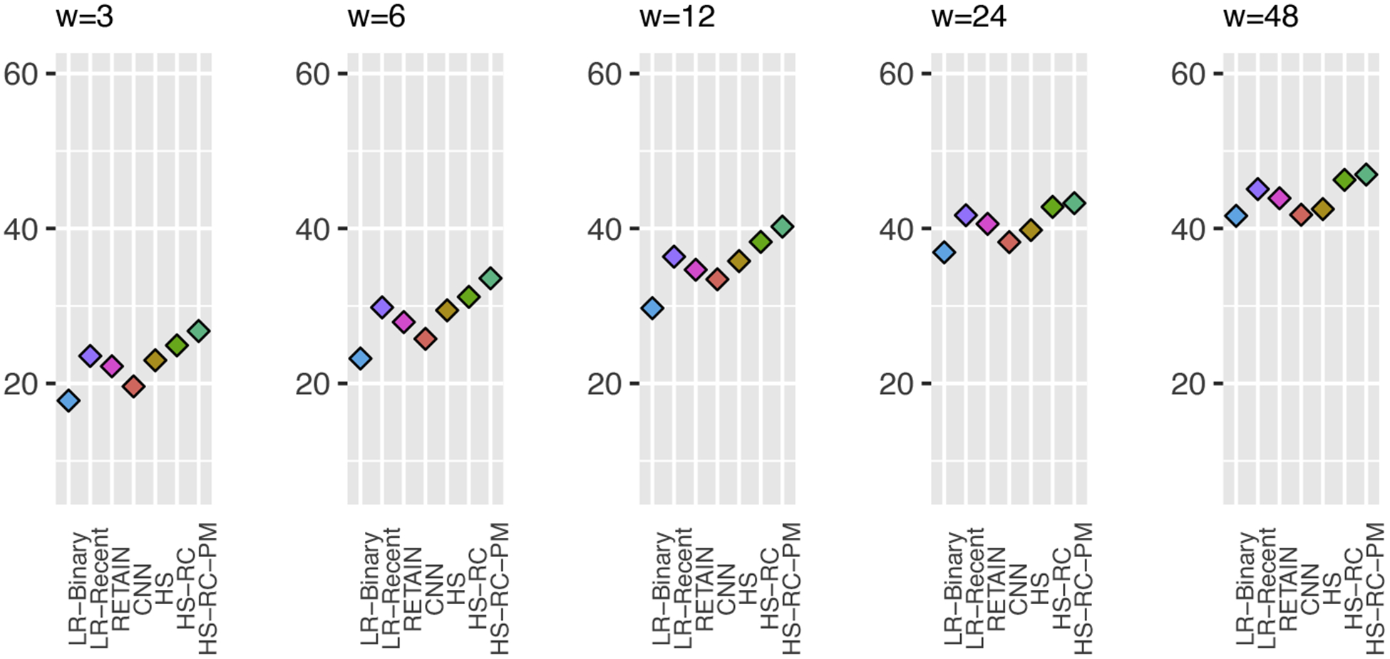
Prediction results for a fixed 12-hour input (segmentation) window, and many different target window sizes.

4.5.4. Statistical Significance of Test Results

To confirm the prediction performance of the proposed method (HS-RC-PM) is different from baseline models, we perform the statistical significance test (T-test) on prediction results (AUPRC) over ten random split runs. As reported in Table 3, the performance of HS-RC-PM is statistically different from all baseline models across all segmentation window settings.

Table 3:

The result of the statistical significance (P-value < 0:05) test (T-test) performed on HS-RC-PM vs. baseline models for AUPRC on 10 random split runs.

W	Baseline model	P-value	Is significant?
6	HS-RC	3.19E-08	TRUE
	HS	5.80E-10	TRUE
	CNN	9.66E-14	TRUE
	RETAIN	5.13E-11	TRUE
	LR-Recent	2.17E-12	TRUE
	LR-Binary	2.47E-16	TRUE
12	HS-RC	7.90E-10	TRUE
	HS	8.02E-16	TRUE
	CNN	1.58E-17	TRUE
	RETAIN	1.83E-17	TRUE
	LR-Recent	2.19E-15	TRUE
	LR-Binary	2.94E-23	TRUE
24	HS-RC	2.34E-09	TRUE
	HS	9.30E-21	TRUE
	CNN	2.22E-20	TRUE
	RETAIN	8.12E-16	TRUE
	LR-Recent	1.87E-11	TRUE
	LR-Binary	8.07E-22	TRUE

5. Conclusion

In this work, we showed the importance of modeling multivariate event time-series with different temporal mechanisms that aim to process different temporal aspects of the time-series. Information on distant past is modeled through the hidden state space defined by LSTM and information on recently observed clinical events is modeled through discriminative projections. We also model periodic (repeated) events using a special external memory mechanism based on probability distributions of inter-event gaps compiled from past data. We show that our model equipped with all the above temporal mechanisms leads to improved prediction performance compared to multiple baselines.

In the future, we plan to extend and test our predictive framework to multistep event predictions. That is, besides predicting events in the next time step y_t+1, we want to predict events in more distant future steps (y_t+2, …, y_t+K). Particularly, we expect the periodicity module could be able to predict multiple future steps accurately with its capability of summarizing recurring events with event gaps. Another refinement we plan to study includes an extension of the neural abstraction module with several improvements. The first is to employ hierarchical LSTM architecture. Recent works on hierarchical temporal models [148, 149, 150] present promising results showing that the hierarchical architecture can successfully model substructures of data. It could help us to model EHR-based event time-series when current events are dependent on different levels of past (e.g., previous hours, the previous part of the day, past weeks, or previous admissions). The second refinement step we consider is to enrich LSTM with extra temporal information such as timings of events and time-of-the-day. As many actions in hospitals take place at specific times (e.g., after morning rounds of clinicians) inclusion of this information in the model may further improve its predictive performance.

Highlights:

• We propose a novel autoregressive event-time-series model that can predict future occurrences of multivariate clinical events.

• Our model represents multivariate event time-series using different temporal mechanisms that aim to process different temporal aspects of the time-series: information about distant past is modeled through the hidden state space defined by an LSTM-based model, information on recently observed clinical events is modeled through discriminative projections, and information about periodic (repeated) events is modeled using a special external memory mechanism based on probability distributions of inter-event gaps compiled from past data.

• We evaluate our proposed model on electronic health record (EHRs) data derived from MIMIC-III dataset and show that our new model equipped with the above temporal mechanisms leads to improved prediction performance compared to multiple baselines.

Appendix A. Hyperparameter Tuning Results

We tune the dimension of hidden states through the internal validation set which is part of training set. As shown in Figure A.13, we report the prediction performances (AUPRC) of models that have hidden states for different window size (W) settings.

Figure A.13:

Predictive performances of models that contain hidden-states on internal validation set, for each window size setting (W=6,12,24)

References

- [1].Yadav P, Steinbach M, Kumar V, Simon G, Mining electronic health records (ehrs) a survey, ACM Computing Surveys (CSUR) 50 (6) (2018) 1–40. [Google Scholar]
- [2].Blumenthal D, Glaser JP, Information technology comes to medicine, The New England journal of medicine 356 (24) (2007) 2527–2534. [DOI] [PubMed] [Google Scholar]
- [3].Chaudhry B, Wang J, Wu S, Maglione M, Mojica W, Roth E, Morton SC, Shekelle PG, Systematic review: impact of health information technology on quality, efficiency, and costs of medical care, Annals of internal medicine 144 (10) (2006) 742–752. [DOI] [PubMed] [Google Scholar]
- [4].Jha AK, DesRoches CM, Campbell EG, Donelan K, Rao SR, Ferris TG, Shields A, Rosenbaum S, Blumenthal D, Use of electronic health records in us hospitals, New England Journal of Medicine 360 (16) (2009) 1628–1638. [DOI] [PubMed] [Google Scholar]
- [5].Johnson AE, Pollard TJ, Shen L, Li-wei HL, Feng M, Ghassemi M, Moody B, Szolovits P, Celi LA, Mark RG, MIMIC-III, a freely accessible critical care database, Scientific data 3 (2016) 160035. [DOI] [PMC free article] [PubMed] [Google Scholar]
- [6].Last G, Penrose M, Lectures on the Poisson process, Vol. 7, Cambridge University Press, 2017. [Google Scholar]
- [7].Ibe O, Markov processes for stochastic modeling, Newnes, 2013. [Google Scholar]
- [8].Rasmussen JG, Lecture notes: Temporal point processes and the conditional intensity function, arXiv preprint arXiv:1806.00221. [Google Scholar]
- [9].Last G, Brandt A, Marked Point Processes on the real line: the dynamical approach, Springer Science & Business Media, 1995. [Google Scholar]
- [10].Jacobsen M, Point process theory and applications: marked point and piecewise deterministic processes, Springer Science & Business Media, 2006. [Google Scholar]
- [11].Liu S, Hauskrecht M, Nonparametric regressive point processes based on conditional gaussian processes, in: Advances in Neural Information Processing Systems, 2019, pp. 1062–1072. [Google Scholar]
- [12].Laub PJ, Taimre T, Pollett PK, Hawkes processes, arXiv preprint arXiv:1507.02822. [Google Scholar]
- [13].Rizoiu M-A, Lee Y, Mishra S, Xie L, A tutorial on hawkes processes for events in social media, arXiv preprint arXiv:1708.06401. [Google Scholar]
- [14].Mei H, Eisner JM, The neural hawkes process: A neurally self-modulating multivariate point process, in: Advances in Neural Information Processing Systems, 2017, pp. 6754–6764. [Google Scholar]
- [15].Nemati S, Holder A, Razmi F, Stanley MD, Clifford GD, Buchman TG, An interpretable machine learning model for accurate prediction of sepsis in the icu, Critical care medicine 46 (4) (2018) 547. [DOI] [PMC free article] [PubMed] [Google Scholar]
- [16].Henry KE, Hager DN, Pronovost PJ, Saria S, A targeted real-time early warning score (trewscore) for septic shock, Science translational medicine 7 (299) (2015) 299ra122–299ra122. [DOI] [PubMed] [Google Scholar]
- [17].Kellum JA, Bihorac A, Artificial intelligence to predict aki: is it a breakthrough?, Nature Reviews Nephrology (2019) 1–2. [DOI] [PMC free article] [PubMed] [Google Scholar]
- [18].Singer M, Deutschman CS, Seymour CW, Shankar-Hari M, Annane D, Bauer M, Bellomo R, Bernard GR, Chiche J-D, Coopersmith CM, et al. , The third international consensus definitions for sepsis and septic shock (sepsis-3), Jama 315 (8) (2016) 801–810. [DOI] [PMC free article] [PubMed] [Google Scholar]
- [19].Bellomo R, Ronco C, Kellum JA, Mehta RL, Palevsky P, et al. , Acute renal failure–definition, outcome measures, animal models, fluid therapy and information technology needs: the second international consensus conference of the acute dialysis quality initiative (adqi) group, Critical care 8 (4) (2004) R204. [DOI] [PMC free article] [PubMed] [Google Scholar]
- [20].Mehta RL, Kellum JA, Shah SV, Molitoris BA, Ronco C, Warnock DG, Levin A, et al. , Acute kidney injury network: report of an initiative to improve outcomes in acute kidney injury, Critical care 11 (2) (2007) R31. [DOI] [PMC free article] [PubMed] [Google Scholar]
- [21].Kdigo A, Work group. kdigo clinical practice guideline for acute kidney injury, Kidney Int Suppl 2 (1) (2012) 1–138. [Google Scholar]
- [22].Hauskrecht M, Valko M, Kveton B, Visweswaran S, Cooper GF, Evidence-based anomaly detection in clinical domains, in: AMIA Annual Symposium Proceedings, Vol. 2007, American Medical Informatics Association, 2007, p. 319. [PMC free article] [PubMed] [Google Scholar]
- [23].Hauskrecht M, Valko M, Batal I, Clermont G, Visweswaran S, Cooper GF, Conditional outlier detection for clinical alerting, in: AMIA annual symposium proceedings, Vol. 2010, American Medical Informatics Association, 2010, p. 286. [PMC free article] [PubMed] [Google Scholar]
- [24].Hauskrecht M, Batal I, Valko M, Visweswaran S, Cooper GF, Clermont G, Outlier detection for patient monitoring and alerting, Journal of biomedical informatics 46 (1) (2013) 47–55. [DOI] [PMC free article] [PubMed] [Google Scholar]
- [25].Hauskrecht M, Batal I, Hong C, Nguyen Q, Cooper GF, Visweswaran S, Clermont G, Outlier-based detection of unusual patientmanagement actions: An ICU study, Journal of Biomedical Informatics 64 (2016) 211–221. [DOI] [PMC free article] [PubMed] [Google Scholar]
- [26].Valko M, Hauskrecht M, Feature importance analysis for patient management decisions, Studies in health technology and informatics 160 (Pt 2) (2010) 861. [PMC free article] [PubMed] [Google Scholar]
- [27].Nguyen Q, Valizadegan H, Hauskrecht M, Learning classification models with soft-label information, Journal of American Medical Informatics Association. [DOI] [PMC free article] [PubMed] [Google Scholar]
- [28].Valizadegan H, Nguyen Q, Hauskrecht M, Learning classification models from multiple experts, Journal of Biomedical Informatics (2013) 1125–1135. [DOI] [PMC free article] [PubMed] [Google Scholar]
- [29].Batal L, Sacchi L, Bellazzi R, Hauskrecht M, Multivariate time series classification with temporal abstractions, in: Proceedings of the 22nd International Florida Artificial Intelligence Research Society Conference, FLAIRS-22, University of Pittsburgh, 2009, pp. 344–349. [Google Scholar]
- [30].Batal I, Valizadegan H, Cooper GF, Hauskrecht M, A temporal pattern mining approach for classifying electronic health record data, ACM Transactions on Intelligent Systems and Technology (TIST) 4 (4) (2013) 1–22. [DOI] [PMC free article] [PubMed] [Google Scholar]
- [31].Batal I, Cooper GF, Fradkin D, Harrison J, Moerchen F, Hauskrecht M, An efficient pattern mining approach for event detection in multivariate temporal data, Knowledge and information systems 46 (1) (2016) 115–150. [DOI] [PMC free article] [PubMed] [Google Scholar]
- [32].Svanström H, Callréus T, Hviid A, Temporal data mining for adverse events following immunization in nationwide danish healthcare databases, Drug safety 33 (11) (2010) 1015–1025. [DOI] [PubMed] [Google Scholar]
- [33].Ji Y, Ying H, Tran J, Dews P, Lau S-Y, Massanari RM, A functional temporal association mining approach for screening potential drug–drug interactions from electronic patient databases, Informatics for Health and Social Care 41 (2016) 387–404. [DOI] [PubMed] [Google Scholar]
- [34].Black W, Temporal data mining in electronic medical records from patients with acute coronary syndrome, Ph.D. thesis (2014).
- [35].Concaro S, Sacchi L, Cerra C, Stefanelli M, Fratino P, Bellazzi R, Temporal data mining for the assessment of the costs related to diabetes mellitus pharmacological treatment, in: AMIA Annual Symposium Proceedings, Vol. 2009, American Medical Informatics Association, 2009, p. 119. [PMC free article] [PubMed] [Google Scholar]
- [36].Boytcheva S, Angelova G, Angelov Z, Tcharaktchiev D, Mining clinical events to reveal patterns and sequences, in: Innovative Approaches and Solutions in Advanced Intelligent Systems, Springer, 2016, pp. 95–111. [Google Scholar]
- [37].Shknevsky A, Shahar Y, Moskovitch R, Consistent discovery of frequent interval-based temporal patterns in chronic patients’ data, Journal of biomedical informatics 75 (2017) 83–95. [DOI] [PubMed] [Google Scholar]
- [38].Sheetrit E, Nissim N, Klimov D, Shahar Y, Temporal probabilistic profiles for sepsis prediction in the icu, in: Proceedings of the 25th ACM SIGKDD International Conference on Knowledge Discovery & Data Mining, 2019, pp. 2961–2969. [Google Scholar]
- [39].Liu Z, Hauskrecht M, A regularized linear dynamical system framework for multivariate time series analysis, in: Twenty-Ninth AAAI Conference on Artificial Intelligence, 2015, pp. 1798–1804. [PMC free article] [PubMed] [Google Scholar]
- [40].Liu Z, Hauskrecht M, Learning linear dynamical systems from multivariate time series: A matrix factorization based framework, in: SIAM International Conference on Data Mining, 2016. [DOI] [PMC free article] [PubMed] [Google Scholar]
- [41].Lasko TA, Denny JC, Levy MA, Computational phenotype discovery using unsupervised feature learning over noisy, sparse, and irregular clinical data, PloS one 8 (6) (2013) e66341. [DOI] [PMC free article] [PubMed] [Google Scholar]
- [42].Schulam P, Wigley F, Saria S, Clustering longitudinal clinical marker trajectories from electronic health data: Applications to phenotyping and endotype discovery, in: Twenty-Ninth AAAI Conference on Artificial Intelligence, 2015. [Google Scholar]
- [43].Liu Z, Wu L, Hauskrecht M, Modeling clinical time series using gaussian process sequences, in: Proceedings of the 2013 SIAM International Conference on Data Mining, SIAM, 2013, pp. 623–631. [Google Scholar]
- [44].Choi E, Bahadori MT, Searles E, Coffey C, Thompson M, Bost J, Tejedor-Sojo J, Sun J, Multi-layer representation learning for medical concepts, in: The 22nd ACM SIGKDD International Conference on Knowledge Discovery and Data Mining, ACM, 2016, pp. 1495–1504. [Google Scholar]
- [45].Farhan W, Wang Z, Huang Y, Wang S, Wang F, Jiang X, A predictive model for medical events based on contextual embedding of temporal sequences, JMIR medical informatics 4 (4) (2016) e39. [DOI] [PMC free article] [PubMed] [Google Scholar]
- [46].Esteban C, Schmidt D, Krompaß D, Tresp V, Predicting sequences of clinical events by using a personalized temporal latent embedding model (2015) 130–139 doi: 10.1109/ICHI.2015.23. [DOI] [Google Scholar]
- [47].Malakouti S, Hauskrecht M, Predicting patient’s diagnoses and diagnostic categories from clinical-events in ehr data, in: Conference on Artificial Intelligence in Medicine in Europe, Springer, 2019, pp. 125–130. [DOI] [PMC free article] [PubMed] [Google Scholar]
- [48].Malakouti S, Hauskrecht M, Not all samples are equal: Class dependent hierarchical multi-task learning for patient diagnosis classification, in: The Thirty-Third International Flairs Conference, 2020. [Google Scholar]
- [49].Choi E, Bahadori MT, Sun J, Kulas J, Schuetz A, Stewart W, Retain: An interpretable predictive model for healthcare using reverse time attention mechanism, in: Advances in Neural Information Processing Systems, 2016, pp. 3504–3512. [Google Scholar]
- [50].Choi E, Bahadori MT, Schuetz A, Stewart WF, Sun J, Doctor ai: Predicting clinical events via recurrent neural networks, in: Machine Learning for Healthcare Conference, 2016, pp. 301–318. [PMC free article] [PubMed] [Google Scholar]
- [51].Jagannatha AN, Yu H, Structured prediction models for rnn based sequence labeling in clinical text, in: Proceedings of the conference on empirical methods in natural language processing. conference on empirical methods in natural language processing, Vol. 2016, NIH Public Access, 2016, p. 856. [DOI] [PMC free article] [PubMed] [Google Scholar]
- [52].Esteban C, Staeck O, Baier S, Yang Y, Tresp V, Predicting clinical events by combining static and dynamic information using recurrent neural networks, in: 2016 IEEE International Conference on Healthcare Informatics (ICHI), Ieee, 2016, pp. 93–101. [Google Scholar]
- [53].Pham T, Tran T, Phung D, Venkatesh S, Predicting healthcare trajectories from medical records: A deep learning approach, Journal of biomedical informatics 69 (2017) 218–229. [DOI] [PubMed] [Google Scholar]
- [54].Lee JM, Hauskrecht M, Recent-context-aware lstm-based clinical time-series prediction, in: In Proceedings of AI in Medicine Europe (AIME), 2019. [DOI] [PMC free article] [PubMed] [Google Scholar]
- [55].Yu K, Zhang M, Cui T, Hauskrecht M, Monitoring icu mortality risk with a long short-term memory recurrent neural network, in: Pac Symp Biocomput, World Scientific, 2020. [PMC free article] [PubMed] [Google Scholar]
- [56].Lee JM, Hauskrecht M, Clinical event time-series modeling with periodic events, in: The Thirty-Third International FLAIRS Conference, AAAI, 2020. [Google Scholar]
- [57].Lee JM, Hauskrecht M, Multi-scale temporal memory for clinical event time-series prediction, in: 2020 International Conference on Artificial Intelligence in Medicine (AIME 2020), 2020. [Google Scholar]
- [58].Lipton ZC, Berkowitz J, Elkan C, A critical review of recurrent neural networks for sequence learning, arXiv preprint arXiv:1506.00019. [Google Scholar]
- [59].Nguyen P, Tran T, Wickramasinghe N, Venkatesh S, Deepr: a convolutional net for medical records, IEEE journal of biomedical and health informatics 21 (1) (2016) 22–30. [DOI] [PubMed] [Google Scholar]
- [60].Rajkomar A, Oren E, Chen K, Dai AM, Hajaj N, Hardt M, Liu PJ, Liu X, Marcus J, Sun M, et al. , Scalable and accurate deep learning with electronic health records, NPJ Digital Medicine 1 (1) (2018) 18. [DOI] [PMC free article] [PubMed] [Google Scholar]
- [61].Hochreiter S, Schmidhuber J, Long short-term memory, Neural computation 9 (8) (1997) 1735–1780. [DOI] [PubMed] [Google Scholar]
- [62].Kingman JFC, Poisson processes, Vol. 3 of Oxford Studies in Probability, The Clarendon Press Oxford University Press, New York, 1993, oxford Science Publications. [Google Scholar]
- [63].MacDonald IL, Zucchini W, Hidden Markov and other models for discrete-valued time series, Vol. 110, CRC Press, 1997. [Google Scholar]
- [64].McKenzie E, Ch. 16. discrete variate time series, Handbook of Statistics 21 (2003) 573–606. doi: 10.1016/S0169-7161(03)21018-X. [DOI] [Google Scholar]
- [65].Hauskrecht M, Batal I, Valko M, Visweswaran S, Cooper GF, Clermont G, Outlier detection for patient monitoring and alerting., Journal of Biomedical Informatics 46 (1) (2013) 47–55. [DOI] [PMC free article] [PubMed] [Google Scholar]
- [66].Stratonovich RL, Conditional Markov processes, Theory of Probability & Its Applications 5 (2) (1960) 156–178. [Google Scholar]
- [67].Rabiner LR, A tutorial on hidden markov models and selected applications in speech recognition, Proceedings of the IEEE 77 (2) (1989) 257–286. [Google Scholar]
- [68].Hassan MR, Nath B, Stock market forecasting using hidden Markov model: a new approach, in: Intelligent Systems Design and Applications, 2005. ISDA’05. Proceedings. 5th International Conference on, IEEE, 2005, pp. 192–196. [Google Scholar]
- [69].Hughey R, Krogh A, Hidden Markov models for sequence analysis: extension and analysis of the basic method, Bioinformatics 12 (2) (1996) 95–107. [DOI] [PubMed] [Google Scholar]
- [70].Smyth P, Clustering sequences with hidden Markov models, in: Advances in neural information processing systems, 1997, pp. 648–654. [Google Scholar]
- [71].Liu Y-Y, Li S, Li F, Song L, Rehg JM, Efficient learning of continuous-time hidden markov models for disease progression, in: Advances in neural information processing systems, 2015, pp. 3600–3608. [PMC free article] [PubMed] [Google Scholar]
- [72].Inaba Y, Shimokawa A, Miyaoka E, Mixed hidden markov models for clinical research with discrete repeated measurements, American Journal of Theoretical and Applied Statistics 6 (6) (2017) 290–296. [Google Scholar]
- [73].Hong C, Hauskrecht M, Analysis of temporal clinical patterns using hidden markov models.
- [74].Stanculescu I, Williams CK, Freer Y, Autoregressive hidden markov models for the early detection of neonatal sepsis, IEEE journal of biomedical and health informatics 18 (5) (2013) 1560–1570. [DOI] [PubMed] [Google Scholar]
- [75].Kalman RE, Mathematical description of linear dynamical systems, Journal of the Society for Industrial and Applied Mathematics 1 (2) (1963) 152–192. [Google Scholar]
- [76].Ghahramani Z, Hinton GE, Parameter estimation for linear dynamical systems, Tech. rep., Technical Report CRG-TR-96–2, University of Totronto, Dept. of Computer Science (1996). [Google Scholar]
- [77].Liu Z, Hauskrecht M, Learning adaptive forecasting models from irregularly sampled multivariate clinical data, in: The 30th AAAI Conference on Artificial Intelligence, 2016, pp. 1273–1279. [PMC free article] [PubMed] [Google Scholar]
- [78].Werbos PJ, Generalization of backpropagation with application to a recurrent gas market model, Neural networks 1 (4) (1988) 339–356. [Google Scholar]
- [79].Hochreiter S, Bengio Y, Frasconi P, Schmidhuber J, et al. , Gradient flow in recurrent nets: the difficulty of learning long-term dependencies (2001).
- [80].Williams RJ, Zipser D, Gradient-based learning algorithms for recurrent, Backpropagation: Theory, architectures, and applications 433. [Google Scholar]
- [81].Sutskever I, Training recurrent neural networks, University of Toronto Toronto, Ontario, Canada, 2013. [Google Scholar]
- [82].Cho K, Van Merriënboer B, Gulcehre C, Bahdanau D, Bougares F, Schwenk H, Bengio Y, Learning phrase representations using rnn encoder-decoder for statistical machine translation, arXiv preprint arXiv:1406.1078. [Google Scholar]
- [83].Han M, Xi J, Xu S, Yin F-L, Prediction of chaotic time series based on the recurrent predictor neural network, IEEE transactions on signal processing 52 (12) (2004) 3409–3416. [Google Scholar]
- [84].Chen P-A, Chang L-C, Chang F-J, Reinforced recurrent neural networks for multi-step-ahead flood forecasts, Journal of Hydrology 497 (2013) 71–79. [Google Scholar]
- [85].Gregor K, Danihelka I, Graves A, Rezende DJ, Wierstra D, Draw: A recurrent neural network for image generation, arXiv preprint arXiv:1502.04623. [Google Scholar]
- [86].Graves A, Jaitly N, Towards end-to-end speech recognition with recurrent neural networks, in: International Conference on Machine Learning, 2014, pp. 1764–1772. [Google Scholar]
- [87].Sutskever I, Vinyals O, Le Q, Sequence to sequence learning with neural networks, (2014) 3104–12. [Google Scholar]
- [88].Bajor JM, Lasko TA, Predicting medications from diagnostic codes with recurrent neural networks, in: ICLR, 2017. [Google Scholar]
- [89].Choi E, Schuetz A, Stewart WF, Sun J, Using recurrent neural network models for early detection of heart failure onset, Journal of the American Medical Informatics Association 24 (2) (2017) 361–370. [DOI] [PMC free article] [PubMed] [Google Scholar]
- [90].Nguyen P, Tran T, Venkatesh S, Finding algebraic structure of care in time: A deep learning approach, ArXiv abs/1711.07980. [Google Scholar]
- [91].Breiman L, Random forests, Machine learning 45 (1) (2001) 5–32. [Google Scholar]
- [92].Suykens JA, Vandewalle J, Least squares support vector machine classifiers, Neural processing letters 9 (3) (1999) 293–300. [Google Scholar]
- [93].Liu Z, Hauskrecht M, Clinical time series prediction: Toward a hierarchical dynamical system framework, Artificial Intelligence in Medicine 65 (1) (2015) 5–18. [DOI] [PMC free article] [PubMed] [Google Scholar]
- [94].Che Z, Purushotham S, Cho K, Sontag D, Liu Y, Recurrent neural networks for multivariate time series with missing values, Scientific reports 8 (1) (2018) 1–12. [DOI] [PMC free article] [PubMed] [Google Scholar]
- [95].Hochreiter S, The vanishing gradient problem during learning recurrent neural nets and problem solutions, International Journal of Uncertainty, Fuzziness and Knowledge-Based Systems 6 (2) (1998) 107–116. [Google Scholar]
- [96].Bahdanau D, Cho K, Bengio Y, Neural machine translation by jointly learning to align and translate, in: 3rd International Conference on Learning Representations, ICLR 2015, 2015. [Google Scholar]
- [97].Britz D, Goldie A, Luong M-T, Le Q, Massive exploration of neural machine translation architectures, arXiv preprint arXiv:1703.03906. [Google Scholar]
- [98].Luong M-T, Pham H, Manning CD, Effective approaches to attention-based neural machine translation, arXiv preprint arXiv:1508.04025. [Google Scholar]
- [99].Xu K, Ba J, Kiros R, Cho K, Courville A, Salakhudinov R, Zemel R, Bengio Y, Show, attend and tell: Neural image caption generation with visual attention, in: International conference on machine learning, 2015, pp. 2048–2057. [Google Scholar]
- [100].Parikh AP, Täckström O Das D, Uszkoreit J, A decomposable attention model for natural language inference, arXiv preprint arXiv:1606.01933. [Google Scholar]
- [101].Paulus R, Xiong C, Socher R, A deep reinforced model for abstractive summarization, arXiv preprint arXiv:1705.04304. [Google Scholar]
- [102].Kim Y, Denton C, Hoang L, Rush AM, Structured attention networks, arXiv preprint arXiv:1702.00887. [Google Scholar]
- [103].Zhang Y, Chen R, Tang J, Stewart WF, Sun J, Leap: learning to prescribe effective and safe treatment combinations for multimorbidity, in: Proceedings of the 23rd ACM SIGKDD International Conference on Knowledge Discovery and Data Mining, ACM, 2017, pp. 1315–1324. [Google Scholar]
- [104].Choi E, Bahadori MT, Song L, Stewart WF, Sun J, Gram: graphbased attention model for healthcare representation learning, in: Proceedings of the 23rd ACM SIGKDD International Conference on Knowledge Discovery and Data Mining, 2017, pp. 787–795. [DOI] [PMC free article] [PubMed] [Google Scholar]
- [105].LeCun Y, Bottou L, Bengio Y, Haffner P, Gradient-based learning applied to document recognition, Proceedings of the IEEE 86 (11) (1998) 2278–2324. [Google Scholar]
- [106].Russakovsky O, Deng J, Su H, Krause J, Satheesh S, Ma S, Huang Z, Karpathy A, Khosla A, Bernstein M, et al. , Imagenet large scale visual recognition challenge, International journal of computer vision 115 (3) (2015) 211–252. [Google Scholar]
- [107].Egmont-Petersen M, de Ridder D, Handels H, Image processing with neural networks—a review, Pattern recognition 35 (10) (2002) 2279–2301. [Google Scholar]
- [108].Nogueira K, Penatti OA, Dos Santos JA, Towards better exploiting convolutional neural networks for remote sensing scene classification, Pattern Recognition 61 (2017) 539–556. [Google Scholar]
- [109].Lopes AT, de Aguiar E, De Souza AF, Oliveira-Santos T, Facial expression recognition with convolutional neural networks: coping with few data and the training sample order, Pattern Recognition 61 (2017) 610–628. [Google Scholar]
- [110].Girshick R, Donahue J, Darrell T, Malik J, Rich feature hierarchies for accurate object detection and semantic segmentation, in: Proceedings of the IEEE conference on computer vision and pattern recognition, 2014, pp. 580–587. [Google Scholar]
- [111].Ren S, He K, Girshick R, Sun J, Faster r-cnn: Towards real-time object detection with region proposal networks, in: Advances in neural information processing systems, 2015, pp. 91–99. [DOI] [PubMed] [Google Scholar]
- [112].Redmon J, Divvala S, Girshick R, Farhadi A, You only look once: Unified, real-time object detection, in: Proceedings of the IEEE conference on computer vision and pattern recognition, 2016, pp. 779–788. [Google Scholar]
- [113].Vinciarelli A, A survey on off-line cursive word recognition, Pattern recognition 35 (7) (2002) 1433–1446. [Google Scholar]
- [114].Jung K, Kim KI, Jain AK, Text information extraction in images and video: a survey, Pattern recognition 37 (5) (2004) 977–997. [Google Scholar]
- [115].Kim I-J, Choi C, Lee S-H, Improving discrimination ability of convolutional neural networks by hybrid learning, International Journal on Document Analysis and Recognition (IJDAR) 19 (1) (2016) 1–9. [Google Scholar]
- [116].Yao K, Yu D, Seide F, Su H, Deng L, Gong Y, Adaptation of context-dependent deep neural networks for automatic speech recognition, in: 2012 IEEE Spoken Language Technology Workshop (SLT), IEEE, 2012, pp. 366–369. [Google Scholar]
- [117].Abdel-Hamid O, A.-r. Mohamed, H. Jiang, G. Penn, Applying convolutional neural networks concepts to hybrid nn-hmm model for speech recognition, in: 2012 IEEE international conference on Acoustics, speech and signal processing (ICASSP), IEEE, 2012, pp. 4277–4280. [Google Scholar]
- [118].Sercu T, Puhrsch C, Kingsbury B, LeCun Y, Very deep multilingual convolutional neural networks for lvcsr, in: 2016 IEEE International Conference on Acoustics, Speech and Signal Processing (ICASSP), IEEE, 2016, pp. 4955–4959. [Google Scholar]
- [119].Collobert R, Weston J, A unified architecture for natural language processing: Deep neural networks with multitask learning, in: Proceedings of the 25th international conference on Machine learning, 2008, pp. 160–167. [Google Scholar]
- [120].Yu L, Hermann KM, Blunsom P, Pulman S, Deep learning for answer sentence selection, arXiv preprint arXiv:1412.1632. [Google Scholar]
- [121].Kalchbrenner N, Grefenstette E, Blunsom P, A convolutional neural network for modelling sentences, arXiv preprint arXiv:1404.2188. [Google Scholar]
- [122].Kim Y, Jernite Y, Sontag D, Rush AM, Character-aware neural language models, in: Thirtieth AAAI conference on artificial intelligence, 2016. [Google Scholar]
- [123].Wang M, Lu Z, Li H, Jiang W, Liu Q, gen cnn: A convolutional architecture for word sequence prediction, arXiv preprint arXiv:1503.05034. [Google Scholar]
- [124].Dauphin YN, Fan A, Auli M, Grangier D, Language modeling with gated convolutional networks, in: International conference on machine learning, JMLR. org, 2017, pp. 933–941. [Google Scholar]
- [125].Razavian N, Marcus J, Sontag D, Multi-task prediction of disease onsets from longitudinal laboratory tests, in: Machine Learning for Healthcare Conference, 2016, pp. 73–100. [Google Scholar]
- [126].Suresh H, Hunt N, Johnson A, Celi LA, Szolovits P, Ghassemi M, Clinical intervention prediction and understanding using deep networks, arXiv preprint arXiv:1705.08498. [Google Scholar]
- [127].Cheng Y, Wang F, Zhang P, Hu J, Risk prediction with electronic health records: A deep learning approach, in: Proceedings of the 2016 SIAM International Conference on Data Mining, SIAM, 2016, pp. 432–440. [Google Scholar]
- [128].Blei DM, Ng AY, Jordan MI, Latent dirichlet allocation, Journal of machine Learning research 3 (Jan) (2003) 993–1022. [Google Scholar]
- [129].Berberidis C, Aref WG, Atallah M, Vlahavas I, Elmagarmid AK, et al. , Multiple and partial periodicity mining in time series databases, in: ECAI, Vol. 2, 2002, pp. 370–374. [Google Scholar]
- [130].Vlachos M, Yu P, Castelli V, On periodicity detection and structural periodic similarity, in: Proceedings of the 2005 SIAM international conference on data mining, SIAM, 2005, pp. 449–460. [Google Scholar]
- [131].Hindle A, Godfrey MW, Holt RC, Mining recurrent activities: Fourier analysis of change events, in: 2009 31st International Conference on Software Engineering-Companion Volume, IEEE, 2009, pp. 295–298. [Google Scholar]
- [132].Jindal T, Giridhar P, Tang L-A, Li J, Han J, Spatiotemporal periodical pattern mining in traffic data, in: Proceedings of the 2nd ACM SIGKDD international workshop on urban computing, ACM, 2013, p. 11. [Google Scholar]
- [133].Osborne MA, Roberts SJ, Rogers A, Ramchurn SD, Jennings NR, Towards real-time information processing of sensor network data using computationally efficient multi-output gaussian processes, in: 2008 International Conference on Information Processing in Sensor Networks (ipsn 2008), IEEE, 2008, pp. 109–120. [Google Scholar]
- [134].HajiGhassemi N, Deisenroth M, Analytic long-term forecasting with periodic gaussian processes, in: Artificial Intelligence and Statistics, 2014, pp. 303–311. [Google Scholar]
- [135].Yuan Q, Shang J, Cao X, Zhang C, Geng X, Han J, Detecting multiple periods and periodic patterns in event time sequences, in: Proceedings of the 2017 ACM on Conference on Information and Knowledge Management, ACM, 2017, pp. 617–626. [Google Scholar]
- [136].Ozden B, Ramaswamy S, Silberschatz A, Cyclic association rules, in: Proceedings 14th International Conference on Data Engineering, IEEE, 1998, pp. 412–421. [Google Scholar]
- [137].Agarwal R, Srikant R, et al. , Fast algorithms for mining association rules, in: Proc. of the 20th VLDB Conference, 1994, pp. 487–499. [Google Scholar]
- [138].Han J, Dong G, Yin Y, Efficient mining of partial periodic patterns in time series database, in: Proceedings 15th International Conference on Data Engineering (Cat. No. 99CB36337), IEEE, 1999, pp. 106–115. [Google Scholar]
- [139].Ma S, Hellerstein JL, Mining partially periodic event patterns with unknown periods, in: Proceedings 17th International Conference on Data Engineering, IEEE, 2001, pp. 205–214. [Google Scholar]
- [140].Cao H, Cheung DW, Mamoulis N, Discovering partial periodic patterns in discrete data sequences, in: Pacific-Asia Conference on Knowledge Discovery and Data Mining, Springer, 2004, pp. 653–658. [Google Scholar]
- [141].Kapoor K, Subbian K, Srivastava J, Schrater P, Just in time recommendations: Modeling the dynamics of boredom in activity streams, in: Proceedings of the Eighth ACM International Conference on Web Search and Data Mining, ACM, 2015, pp. 233–242. [Google Scholar]
- [142].Trouleau W, Ashkan A, Ding W, Eriksson B, Just one more: Modeling binge watching behavior, in: Proceedings of the 22nd ACM SIGKDD International Conference on Knowledge Discovery and Data Mining, ACM, 2016, pp. 1215–1224. [Google Scholar]
- [143].Kurashima T, Althoff T, Leskovec J, Modeling interdependent and periodic real-world action sequences, in: Proceedings of the 2018 World Wide Web Conference on World Wide Web, International World Wide Web Conferences Steering Committee, 2018, pp. 803–812. [DOI] [PMC free article] [PubMed] [Google Scholar]
- [144].Adar E, Teevan J, Dumais ST, Large scale analysis of web revisitation patterns, in: Proceedings of the SIGCHI conference on Human Factors in Computing Systems, ACM, 2008, pp. 1197–1206. [Google Scholar]
- [145].Werbos PJ, Backpropagation through time: what it does and how to do it, Proceedings of the IEEE 78 (10) (1990) 1550–1560. [Google Scholar]
- [146].Kingma DP, Ba J, Adam: A method for stochastic optimization, arXiv preprint arXiv:1412.6980. [Google Scholar]
- [147].Saito T, Rehmsmeier M, The precision-recall plot is more informative than ROC plot when evaluating binary classifiers on imbalanced datasets, PloS One 10 (3) (2015) e0118432. [DOI] [PMC free article] [PubMed] [Google Scholar]
- [148].Chung J, Ahn S, Bengio Y, Hierarchical multiscale recurrent neural networks, arXiv preprint arXiv:1609.01704. [Google Scholar]
- [149].Kádár A, Côté M-A, Chrupal a G, Alishahi A, Revisiting the hierarchical multiscale lstm, arXiv preprint arXiv:1807.03595. [Google Scholar]
- [150].Zhang T, Huang M, Zhao L, Learning structured representation for text classification via reinforcement learning, in: Thirty-Second AAAI Conference on Artificial Intelligence, 2018. [Google Scholar]