

Abstract
Inverse Ising inference is a method for inferring the coupling parameters of a Potts/Ising model based on observed site-covariation, which has found important applications in protein physics for detecting interactions between residues in protein families. We introduce Mi3-GPU (“mee-three”, for MCMC Inverse Ising Inference) software for solving the inverse Ising problem for protein-sequence datasets with few analytic approximations, by parallel Markov-Chain Monte-Carlo sampling on GPUs. We also provide tools for analysis and preparation of protein-family Multiple Sequence Alignments (MSAs) to account for finite-sampling issues, which are a major source of error or bias in inverse Ising inference. Our method is “generative” in the sense that the inferred model can be used to generate synthetic MSAs whose mutational statistics (marginals) can be verified to match the dataset MSA statistics up to the limits imposed by the effects of finite sampling. Our GPU implementation enables the construction of models which reproduce the covariation patterns of the observed MSA with a precision that is not possible with more approximate methods. The main components of our method are a GPU-optimized algorithm to greatly accelerate MCMC sampling, combined with a multi-step Quasi-Newton parameter-update scheme using a “Zwanzig reweighting” technique. We demonstrate the ability of this software to produce generative models on typical protein family datasets for sequence lengths L ~ 300 with 21 residue types with tens of millions of inferred parameters in short running times.
1. Introduction
The inverse Ising problem consists of finding the set of “coupling” parameters of an Ising or Potts model which reproduce observed site-covariation of the Potts system in thermodynamic equilibrium. It has many practical applications in computer vision, machine learning and biophysics to detect interaction networks among large collections of covarying components, each of which can take on a set of discrete values, and the Potts or Ising models parameterized by this method are also known by the names of Markov Random Fields and graphical models. An important application of inverse Ising inference is for “protein covariation analysis”, by which one detects interactions between residues within proteins based on observed mutational covariations in multiple sequence alignments (MSAs) of proteins from a common protein family, which arise during the course of evolution through compensatory effects [1, 2, 3, 4, 5, 6, 7]. These predicted interactions have been found to correspond well to physical contacts within the 3D structure of proteins, and models inferred from protein sequence data have shown great promise for elucidating the relationship between protein sequence, structure and function [8, 9, 10, 11, 12].
The inverse Ising problem is a difficult computational challenge. A Potts model describes the likelihood of configurations S = s1, s2…sL of L “sites” or positions, each of which can take one of q states. Solving the inverse problem exactly by naive means involves sums over all qL possible configurations, which quickly becomes computationally infeasible for increasing values of L. This has motivated a variety of approximate solution methods including message passing [13], mean-field approximations [14], pseudolikelihood approximations [10], and adaptive cluster expansion [15, 16]. However, these approximations often introduce biases into the inferred model parameters which can cause the site-covariances of sequences or MSAs generated by the model to differ from those obtained using inference approaches that employ fewer approximations, meaning the model is not “generative” and cannot be used in certain applications involving evaluation of sequence-by-sequence statistical predictions [17, 16]. The inverse Ising problem can be solved with fewer analytic approximations using Markov-Chain Monte-Carlo (MCMC) sampling methods [2, 18, 19], but these are limited by the requirement of Markov-Chain convergence and by the effects of finite sampling error due to limited configuration sample size, and this approach is typically much more computationally demanding.
The software presented here provides a GPU-accelerated MCMC inverse Ising inference strategy (“Mi3”, for MCMC Inverse Ising Inference), focusing on the application of protein covariation analysis with high statistical accuracy, and is implemented in the Python and OpenCL programming languages. It uses large Monte-Carlo sample sizes to limit finite-sampling error and bias. The main components of this method are a GPU-optimized algorithm for MCMC sampling, combined with a multi-step Quasi-Newton parameter-update scheme [20] using a “Zwanzig reweighting” strategy [21, 22, 23, 24] which allows many parameter update steps to be performed after each MCMC sample. With this method we can obtain statistically accurate and generative models for large Potts systems, allowing detailed analysis of sequence and MSA statistics which is otherwise difficult [25, 24, 26, 27]. We demonstrate its performance by fitting a protein family with sequences of length L = 232 and q = 21 residue types (20 amino acids plus gap), to parameterize a Potts model with 12 million parameters in a reasonable running time. This problem size is typical of protein family datasets for covariation analysis from the Pfam database, which are commonly L ~ 200 and q = 21.
The statistically accurate model and marginals produced by this method are particularly suited for studying sequence variation on a sequence-by-sequence basis and detailed MSA statistics related to higher order marginals, but can also be used in other common applications of covariation analysis. We illustrate some applications in Fig. 1. We have previously used initial versions of the Mi3-GPU software to perform analysis difficult using more approximate methods. For instance, we have used this method to test whether pairwise terms are necessary and sufficient to model sequence higher-order marginals, by showing that sequences generated by the model have similar higher-order marginals as those of the dataset [25] using our accurate marginal estimates, as in Fig. 1B, bottom. We have also used it to show how mutations leading to drug resistance in HIV can become highly favored (or entrenched) by the complex mutation patterns arising in response to drug therapy despite being disfavored in the wild-type sequence background [26], and we used these statistically accurate models to predict which mutations a particular background will support and how conducive that background is towards that mutation [29], as illustrated in Fig. 1D. This fitting procedure was also key to an analysis on the effects of overfitting and the statistical power of Potts models [27], in which we demonstrated the resilience of the inference procedure to the statistical error caused by finite-sampling effects due to the limited size of the dataset MSA, and estimated how many sequences are necessary to accurately construct a model, as illustrated in figure 1C. The statistical accuracy of the method allowed estimation of the statistical error of various model predictions, such as prediction the effects of point mutations and double mutant effects.
Figure 1:
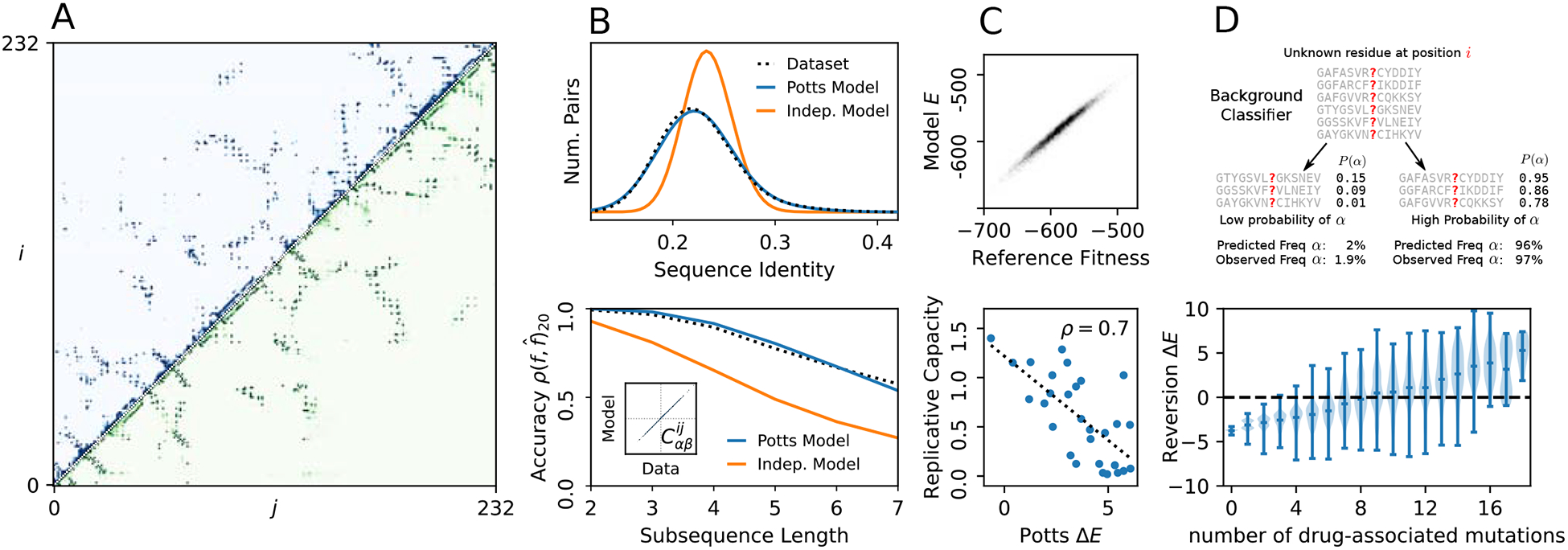
Example applications of covariation analysis possible using Mi3-GPU. (A) Example of contact prediction in protein structure for the protein family used in this study. Dark points in the upper triangle of this contact map are i, j pairs with a strong Potts interaction score predicted using Mi3-GPU. The lower triangle shows contact frequency observed in structures in the PDB with a 6Å side-chain cutoff distance, with excellent agreement. (B) The models inferred by this method accurately reconstruct MSA statistical properties which are not directly fit. Top: The distribution of Hamming distances between all pairs of sequences in an MSA generated by the model is the same as for the dataset MSA and unlike that of an MSA generated using a site-independent model. Bottom: MSAs generated from the model reproduce the higher-order marginals (subsequence frequencies) in the data as far as finite-sampling limitations allow us to verify. This suggests the sufficiency of pairwise Potts models to model protein sequence variation, as discussed in Ref. [25]. The y-axis reflects the average Pearson correlation in model marginal predictions with dataset marginals. The estimated finite-sample verification limit is shown in black as in Ref. [25]. Inset: The pairwise residue covariations are very accurately reproduced in generated sequences. (C) Top: A Potts model fit to only 10,000 sequence generated from a “reference” model predicts their fitnesses (statistical energy) compared to the reference fitness, showing that our method is resilient to finite-sampling errors as discussed in ref [27]. Bottom: Potts computations of mutation effects in HIV protease predict experimental replicative capacity measurements from Ref. [28] as discussed in Ref. [26]. (D) Potts models predict complex background-dependent statistics of individual sequences. Top: The Potts model can classify which sequences are likely to have a particular residue at a position based on knowledge of the rest of the sequence, discussed in Ref. [29], and accurately predicts the observed residue frequencies in each classified sequence group. Bottom: The Potts model predicts the bias for of reversion of a primary drug-resistance mutants in HIV protease sequences due to accessory drug-resistance mutations by computing the statistical energy change ΔE caused by reversion, as discussed in Ref. [26]. In sequences with ΔE > 0 the drug-resistance mutation is “entrenched” and difficult to revert.
We also address the sources of error and bias in the inference procedure and describe MSA preprocessing tools we provide to account for them. Finite sampling error caused by limited dataset size is a fundamental source of error in protein covariation analysis and more generally for inverse Ising inference on real datasets, and causes various problems including overfitting [27]. A careful understanding of the effects of finite sampling error is particularly important when using MCMC methods and Zwanzig reweighting as these explicitly use finite samples of synthetic sequences [15, 27, 30, 31].
2. Background: Inverse Ising Inference
A Potts model describes configurations of sets of L elements {si} taking q possible values. In models representing ferromagnets, q = 2 and the elements represent “spins”, while in protein covariation analysis each configuration represents a protein sequence S of length L where each character is one of q = 21 amino acid or gap characters. The Potts system is described by the Hamiltonian
| (1) |
with “coupling” parameters between all pairs of positions i, j for all characters α, β and “field” parameters for all positions. The probability of observing the sequence S in equilibrium is with normalization constant . This model is in principle “infinite range”, meaning all pairs of elements may be coupled, and each of the coupling and field values may be different.
The Potts model can be motivated by the fact that it is the maximum-entropy model for the probability distribution P(S) of sequences in a protein-family with the constraint that the pairwise (bivariate) amino acid probabilities predicted by the model are equal to frequencies measured from a dataset MSA of N sequences. By capturing the bivariate marginals, we also capture the pairwise residue covariances . The fact that there are no third or higher-order terms in the Hamiltonian of Eq. 1 is a consequence of the choice to only constrain up to the bivariate amino-acid probabilities, and this effectively assumes there are no interaction terms higher than second order. There is evidence this assumption is both necessary sufficient to model some protein-sequence data [25]. Given an MSA of sequence length L and alphabet of q letters, there are bivariate frequencies used as model constraints, although because the univariate frequencies must be consistent across all pairs and sum to 1 the constraints are not independent, and can be reduced to bivariate plus L(q − 1) univariate independent constraints. Maximizing the entropy with these constraints leads to an exponential model with the Hamiltonian of Eq. 1. We refer to Refs. [32, 2, 8, 10] for additional development and motivation for this maximum entropy derivation.
There is a convenient simplification of Eq. 1, which is motivated through the maximum entropy derivation of the Potts model. The number of independent constraints on the marginals, , must equal the resulting number of free parameters of the model, yet in the formulation of Eq. 1 we defined model parameters which means that of these must be superfluous. Indeed one can apply “gauge transformations” for arbitrary constants and this only results in a constant energy shift of all sequences and does not change the probabilities P(S). The model can be fully specified using the same number of parameters θ as there are independent marginal constraints by fixing the “gauge” and eliminating certain coupling and field parameters. In particular it is possible to apply gauge transformations which set all fields to 0 by the gauge transformations with . This simplifies the mathematical formalism of the Potts model and allows simpler and shorter implementation of the MCMC inference algorithm, and from this point we will drop the field terms from all equations, and compute the statistical energy as , and we avoid having to store and handle the field parameters in our implementation. This “fieldless” gauge transformation only eliminates Lq of the superfluous parameters and further elimination is possible, however in practice we find the remainder are difficult to eliminate in such a convenient way. The Mi3-GPU software includes a helper script to transform model parameters between a number of commonly used gauges.
The “inverse” problem of solving for the Potts parameters which satisfy the constraints with given is challenging because of the notoriously difficult problem of calculating the partition function Z or of performing the “forward” computation of , since these both involve a sum over qL sequences S (unique configurations). This has motivated the various approximate inference strategies noted above, for instance in the pseudolikelihood method the partition function is replaced by an approximate partition function which is analytically tractable. Monte-Carlo methods are another popular approach to estimating partition functions and average values such as , and there is a long history and a wealth of literature on using MCMC for this purpose for Ising/Potts systems [33]. MCMC has the advantage noted above that it does not involve analytic approximations, but it is computationally costly. A goal of our inference software is to optimize inverse Ising inference by MCMC.
3. Algorithm Overview
The goal of the Mi3-GPU software is to identify the coupling parameters which satisfy the constraint equations . where are the model bivariate marginals and are the fixed bivariate marginals computed from the dataset MSA. Using a quasi-Newton method we solve for the root of the constraint equations, which we show below leads to a coupling-update relation
| (2) |
in the fieldless gauge, where γ is a parameter controlling the step size and are the updated coupling parameters, and are the trial coupling parameters. Iterating this coupling-update equation leads to values of the coupling parameters which satisfy the constraint once the algorithm converges. The model bivariate marginals are needed to evaluate the coupling-update, which we estimate by Monte-Carlo sampling given the trial couplings. The Mi3-GPU software performs these computations in two phases as outlined in Fig. 2: First, a sequence generation phase in which a “synthetic” MSA is generated by MCMC given a set of trial couplings, from which we calculate . Second, a parameter update phase in which the trial couplings are updated using Eq. 2. The algorithm is initialized with an initial guess for the trial couplings J0 based on the dataset MSA and the two phases are iterated until parameter convergence, which is detected using diagnostics we describe below. We will give a high level overview of these two phases here, and we will elaborate with details in subsequent sections.
Figure 2:
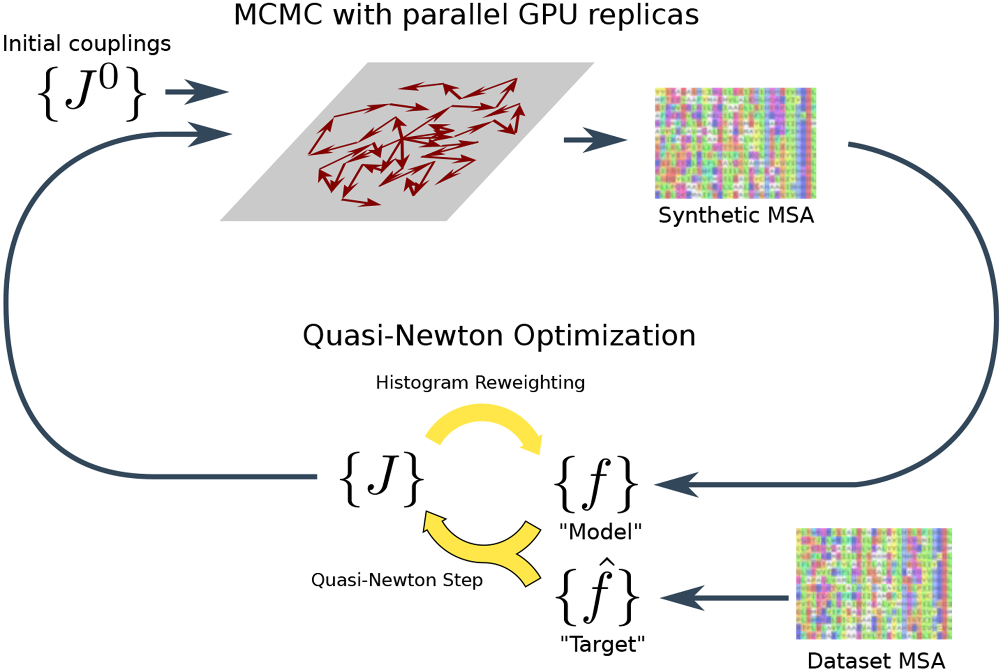
Schematic of the computational strategy used by Mi3-GPU for inverse Ising inference. The algorithm alternates between a sequence generation phase (top of diagram) and a parameter-update phase (bottom of diagram). See text for details.
In the MCMC phase of the inference we aim to efficiently generate a set of N sample sequences from the distribution P(S|J) given trial model parameters J. The MCMC phase is the main bottleneck of the overall algorithm, and the typical number of samples N is large, on the order of N = 104 to 107, for statistical accuracy of the estimated bivariate marginals. The underlying MCMC methodology is a straightforward application of the Metropolis-Hastings algorithm using attempted point-mutations (single-character changes), but accelerated for GPUs. A GPU is able to run a large number of “threads” in parallel, and we arrange for each thread to carry out a Markov chain walk for a single sequence, so that the number of generated sequences equals the number of threads. In each MC step each GPU walker attempts a random single-character change causing a change in Potts statistical energy ΔE between the initial sequence and the modified sequence, which is used to calculate the Metropolis-Hastings acceptance probability, min(1, e−ΔE). All threads on the GPU perform an equal number of Markov steps until we have detected that the Markov chains have converged to the equilibrium distribution, using a convergence diagnostic described below which tests for mixing of the chain energies E(S) relative to each other at two time-points. The output of this phase is a set of N statistically independent sequences drawn from the distribution P(S|J), from which we estimate .
In the second phase we update the trial coupling parameters J based on the discrepancy between the dataset MSA bivariate marginals and those of the synthetic MSA, using Eq. 2. After updating the couplings we could use these in the next phase of MCMC sequence generation, but this would be computationally prohibitive because of the computational cost of the MCMC sequence generation. Instead we use a “Zwanzig reweighting” method to repeatedly compute updated bivariate marginals based on the new couplings without generating a new synthetic MSA. In this method the updated couplings are used to assign weights wn to each sequence in the synthetic MSA based on the energy of that sequence under the new Hamiltonian, chosen so that weighted averages approximate thermodynamic averages under the updated Potts Hamiltonian. This allows us to estimate the marginals under the new Hamiltonian. This allows many coupling-update steps to be computed per MCMC sequence generation run, in practice for hundreds or thousands of iterations. This reweighting technique becomes less accurate once the updated coupling parameters become different enough from those used to generate the synthetic MSA according to criteria we discuss below, at which point we generate a new synthetic MSA using MCMC.
3.1. MCMC sequence generation
Here we describe the MCMC algorithm for GPUs in more detail. A GPU contains many cores which can run a large number of “threads” in parallel to perform a computation, and as described above we have each thread carry out a MCMC walk for a single sequence using the Metropolis-Hastings algorithm. Mi3-GPU can use multiple GPUs in parallel across multiple compute-nodes using the MPI (Message Passing Interface) standard. We use the mwx64x random number generator library for OpenCL to generate trial mutant residues and evaluate acceptance [34].
The main optimization of our implementation is to harness GPU hardware for increased parallelization in calculating ΔE for all sequences in each MC step needed to evaluate the Metropolis probability, as this is the computational bottleneck of our algorithm. GPUs have a much larger number of parallel processors than CPUs, but also have much higher memory bandwidth to feed data to the processors and increased opportunity for data-sharing among processors. When implementing a parallel algorithm for GPUs one can make choices which rebalance processor workload versus data transfer requirements, for instance by tuning data-sharing among processors and arranging for optimized memory access patterns, and this is what we have done for the ΔE calculation. As is typical of GPU software, ours is limited by the memory access speed rather than by the arithmetic processor speed, and our main optimizations are in memory access. Our implementation does not change the computational complexity of the MCMC algorithm, rather it is a parallelization using GPU hardware.
To perform a MCMC step for all N sequences, for each sequence S the value of ΔE is computed in a fieldless gauge as a sum over L − 1 coupling change values as
| (3) |
for a mutation to residue α at position i. In order to evaluate ΔE for all N sequences in each MCMC step, a naive implementation would require loading L − 1 coupling parameters , which are semi-randomly distributed among all couplings, and L sequence characters sj for all N walkers, which can add up to many Gb. We mitigate this on the GPU through optimized memory access. A GPU contains memory locations including a large pool of “global” memory (often many Gb) with high memory-access latency and small amount of “local” memory (often less than 100 Kb) with much lower access latency which can be shared among GPU processors. Parameters such as the values must be loaded from global memory before they can be used in computations.
Key to our GPU implementation’s performance is the choice to simultaneously mutate the same position in all sequences in each step, rather than mutate different random positions in each sequence, as this allows for significant data-sharing between processors as well as other memory-access optimizations. Specifically, this allows threads on a GPU to share the coupling values involving the mutated position in GPU local memory. For each of the L − 1 terms of the sum in Eq. 3 only the q2 coupling values corresponding to position-pair i, j are needed to evaluate all sequences at once, which is small enough to share in the GPU’s local memory to share among processors. Additionally, this data-sharing strategy allows a GPU memory-access optimization known as “latency hiding”. GPU threads are divided into “work groups”, in our case into 512 threads per group. When the local memory requirement per work-group is low, as it is here, the GPU can run more work-groups in parallel at once leading to higher “GPU occupancy” and the GPU can interleave memory transfers from the GPU’s global memory to local memory for some work-groups with computation by other work-groups, which hides the global memory access latency. Another important GPU optimization is “memory coalescing” which reduces memory latency when consecutive threads in a work-group load consecutive elements of global memory to local memory. By using a fieldless gauge and appropriate memory layout, our data-sharing strategy allows the memory transfer of the coupling parameters to be carried out in a highly coalesced manner. The character sj in Eq. 3 can also be loaded in a coalesced manner by all work-units after transposing the MSA in memory so that consecutive memory addresses represent the same position in all sequences, i.e. the MSA is represented as an L × N buffer where the N axis is the “fast” (consecutive) axis.
The fact that the same position is mutated in all walkers raises the question of whether statistical coupling is introduced between the walkers, which would bias our results if this led to non-independent samples of the distribution P(S). It can be seen that there is no such statistical coupling by considering two walkers evolving over the joint sequence state-space (S1, S2) by point mutations. In each step each walker individually attempts a mutation at the same random position i to a different random residue with q possibilities, and the two moves are separately accepted using the Metropolis-Hastings criterion. The joint-state of the outcome may be (S1, S2), , , or for all q2 possible values of α and β, where is the first walker’s sequence mutated at position i to residue α. This is a subset of the possibilities if the two walkers were allowed to mutate different positions i, j with outcome states (S1, S2), , , or for all α, β, and one finds that the ratio of the forward and backward Metropolis rates from each of the restricted (same-position) final states to the initial state is the same in both schemes. Since we have a conservative potential and both schemes are ergodic, they reach equilibrium satisfying detailed balance with equal rate-ratios and therefore equal equilibrium probabilities, which in the second scheme clearly involves no correlations between walkers.
The MCMC step is Input-Output-bound by the memory transfers of the coupling parameters and sequence characters from GPU global to local memory. In order to evaluate a single MCMC step for all sequences a total of LN sequence characters (1 byte each) are loaded using coalesced loads of 4-byte words, and Lq2 coupling values (4 bytes each) are loaded per work-group using coalesced loads, and the number of work-groups is N/w for work-group size w, for a total transfer of 4NLq2/w bytes for the coupling parameters. The value of w affects GPU performance independently of this Input-Output analysis by controlling GPU data-sharing and occupancy, and due to program constraints we require it to be a power of 2. We find w = 512 is optimal in our tests. This gives a total transfer requirement amortized per GPU-walker (divided by N) of L + 4Lq2/w bytes per MCMC step.
In Fig. 3 we benchmark the MCMC sequence generation phase for varied combinations of L, q, N on a single NVidia V100 GPU. We use randomly generated coupling parameters, but have tested with other coupling parameters and find this choice does not noticeably affect the running time. We fit these data by least-squares to the functional aL + b(4Lq2/w) with two free scaling parameters a, b reflecting the speed of the sequence character transfers and coupling-parameter transfers respectively, which we expect to be differently affected by GPU memory access behavior. We find an excellent fit with a = 4.2×10⁻¹² s/step, b = 3.1×10⁻¹² s/step. There is some variation due to difficult-to-predict GPU occupancy and caching effects for different system sizes.
Figure 3:
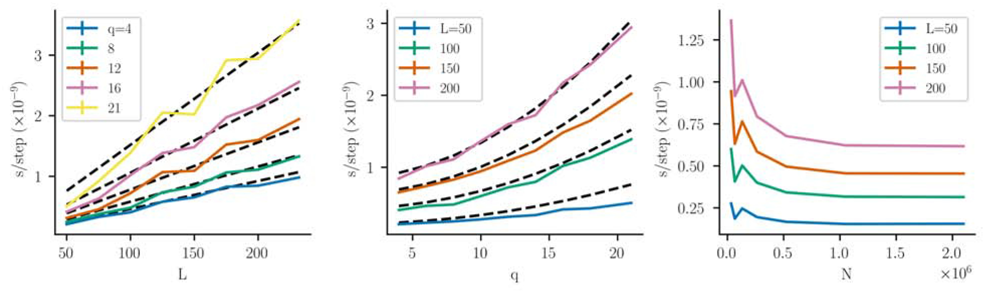
Performance of MCMC sequence generation as a function of L, q and N on an NVidia V100 GPU, measured as the amortized MCMC step running time per GPU-walker. Each datapoint (colored lines) is an average of 3 runs, and the error bars are too small to see. The dotted black lines show a least-squares fit to the expected memory transfer requirements (see text). (A) The running time per walker increases linearly with L, and (B) weakly quadratically with q, where in these panels N is held fixed at N ~ 2 × 10⁶, and very similar results are obtained for smaller values of N. (C) The amortized running time per walker levels off to its minimum for large N with where the MCMC generation is most efficient, using q = 16.
Additionally, for large number of walkers N we expect GPU occupancy will be high and the amortized time per walker will not depend on the number of walkers N, which we observe in Fig. 3C. At small N the amortized time per walker increases, suggesting lower occupancy and inefficient use of the GPU. This has implications for how to divide work among GPUs when multiple GPUs are available. Distributing a fixed amount of walkers among a greater number of GPUs allows more walkers to be iterated in parallel, but there are diminishing returns to using more GPUs as the number of walkers per GPU becomes low and GPU occupancy decreases. For typical protein lengths, Fig. 3C suggests that using about 104 or fewer walkers per GPU leads to inefficient GPU usage. Because it is best to use a number of walkers which are a power of 2 to maximize GPU occupancy, we recommend arranging to use 215 or more walkers per available GPU.
We compare these running times to equivalent running times on CPUs. For the same sets of parameters, we run MCMC with a nearly identical parallelized algorithm on CPUs, including the same-position optimization using shared memory which also optimizes memory access on CPUs. Running on a 20-core Intel(R) Xeon(R) CPU E5–2660 v3 @ 2.60GHz using 2133 MHz DDR4 memory, we find an average speedup of 90x in amortized s/step on the GPU compared to the CPU (Fig. 4). The smallest speedup was 46x for the smallest system for q = 4, and the largest speedup was 247x for q = 21, L = 200, which is more typical of systems studied using protein covariation analysis. The CPU timings increase dramatically for certain large q and L such as L = 200, q > 12, which may be due to caching issues as the storage size of the coupling parameters begins to exceed the size of the caches on the processor used in these tests. These large system sizes are the ones commonly of interest for protein family analysis.
Figure 4:
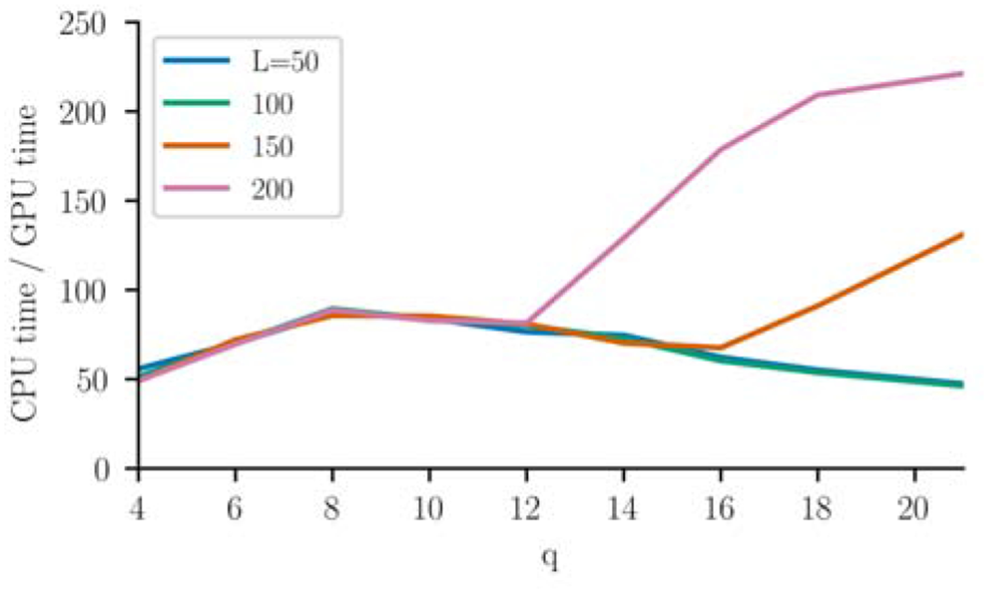
Performance of the MCMC phase of the algorithm on the GPU compared to the CPU, computed as the CPU to GPU ratio of the amortized MCMC step running times, using N ~ 2 × 10⁶.
3.2. MCMC Convergence
In order to obtain independent samples from the distribution P(S) from each GPU walker, we must run enough MCMC steps for the system to reach a Markov equilibrium. Determining how long to run an MCMC simulation so that it has converged is a difficult problem [35, 36, 37, 38]. We estimate MCMC convergence by measuring the inter-walker lag-t/2 autocorrelation of the walker energies, ρ({E(t)}, {E(t/2)}), where {E(t)} is the vector of N walker energies at time t, as illustrated in Fig. 5. We stop when the p-value of the null (uncorrelated) expectation of ρ estimated using a Gaussian approximation is greater than a cutoff, of 0.2 by default. This strategy takes advantage of the fact that our implementation runs a large number (often 104 to 107) MC walkers in parallel, and involves both within-chain contrasts (the energy of a MCMC chain at two different points) and between-chain contrasts (the energy of different chains) which helps avoid issues with convergence diagnostics that only depend on one of these [36]. Convergence is detected when the p-value is high, so that the within-chain energy variations are similar to the cross-chain variations. This diagnostic imposes negligible additional computational cost and only requires recording the sequence energies at half the number of steps.
Figure 5:
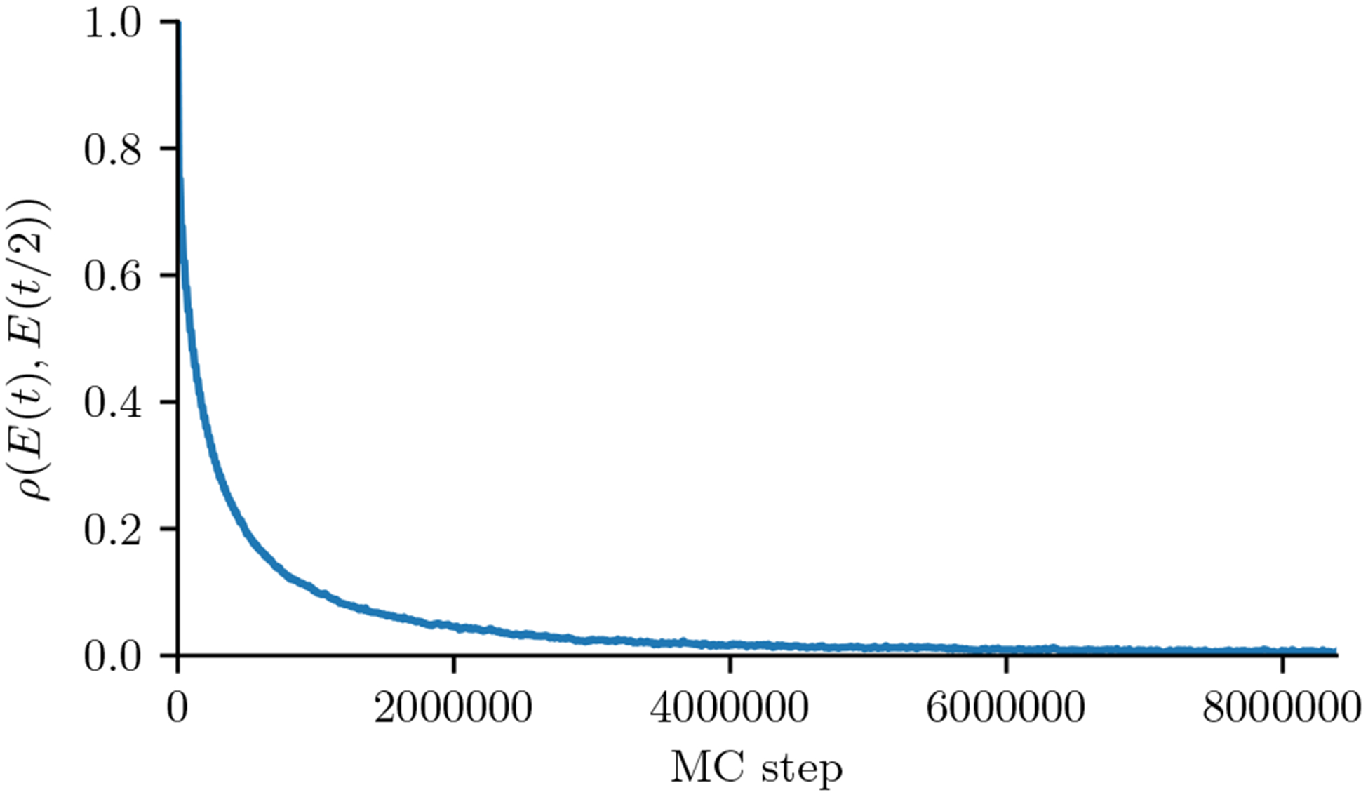
Autocorrelation ρ({E(t)}, {E(t/2)}) of the walker energies for a Kinase Potts model as a function of Monte Carlo step, which we use a convergence diagnostic. Convergence is detected once the p-value of the correlation reaches 0.2, which occurs at the right end of this plot. The number of sequence energies is N ~ 106.
We note that our MCMC-sampling scheme does not use enhanced-sampling methods such as parallel-tempering or Swendsen-Wang algorithm which can be important for obtaining convergence of Ising systems near or below a critical effective temperature. We have found that protein-family sequence data such as obtained from the Pfam database can be accurately fit to Potts models in the high-temperature phase.
4. Quasi-Newton Optimization
After a synthetic MSA has been generated by MCMC, in the parameter update phase we update the coupling parameters of the model using Eq. 2, which we derive here. We use a quasi-Newton approach to find the root of the constraint equation Δf = 0, following previous methodology [20, 24] but using a different “pairwise” approximation leading to the new coupling update equation in Eq. 2. The expected change in marginals df due to a change in couplings dJ is given to first order by
| (4) |
and by inverting this linear equation we can solve for the step dJ which would give a desired df, as . This requires inverting the Jacobian matrix whose elements can be found from the definition of to be
| (5) |
where is a 4th-order marginal, which reduces to lower order marginals in the cases where the upper indices are equal to each other, and equals 0 in the case that two upper indices are equal but the corresponding lower indices are different. This Jacobian is a non-sparse by matrix, and is too large to invert numerically in a reasonable time.
To invert it we resort to a pairwise approximate inversion, by assuming that residues at each pair of positions varies independently of other position-pairs so that each bivariate marginal depends only on the couplings at the same positions for all α, β, and all other off-diagonal elements in the Jacobian are 0. This reduces the problem to a set of independent pair (L = 2) systems, and in this section we drop the i, j indices. In the L = 2 system there are q2 − 1 independent marginals (i.e., all but one of the bivariate marginals due to normalization ∑ fαβ = 1), and in the fieldless gauge there are q2 couplings, and thus one superfluous parameter. Then Eqs. 5 and 4 simplify to
| (6) |
and by rearranging we find this is solved (up to a constant due to the gauge freedom) by
| (7) |
We set with step-size factor γ chosen small enough for the linear approximation to be valid. This step will reduce the discrepancy between the dataset bivariate marginals and the model marginals, and will lead to the optimized solution when iterated. Substituting this into Eq. 7 gives the coupling-update relation of Eq. 2.
In practice, we also modify the step direction by adding an extra damping parameter to Eq. 2 to prevent large step-sizes for coupling parameters corresponding to small sampled values of fαβ in the denominator, as Eq. 7 diverges as fαβ → 0. Such large steps would move the parameters outside the range of linear approximation we are using, and can prevent smooth progress towards the solution. The damping modification is equivalent to adding flat pseudocount p to the bivariate marginals, giving pseudocounted marginals , and substituting these for fαβ in Eq. 7 to obtain a modified step direction
| (8) |
This damped step direction leads to the same solution as the undamped step direction, since if Δfαβ = 0 then and dJαβ = 0, and the inferred solution Jαβ will be independent of p. This damping reduces the step size for couplings corresponding to small marginals where divergence of Eq. 7 is more likely. We find that it is useful to use a higher value for p such as 0.01 when the system is far from the solution, and as the system approaches the solution and the typical step sizes becomes smaller p can be decreased.
4.1. Zwanzig Reweighting
The marginals required in the update step of Eq. 2 must be determined from a computationally demanding MCMC sequence-generation run, but using a Zwanzig reweighting approach we evaluate the marginals for small changes in couplings without regenerating a new set of sequences, allowing many more approximate coupling update steps per round of MCMC generation [21, 22, 23, 24]. Zwanzig reweighting methods use the fact that a thermodynamic average under one Hamiltonian is equal to a weighted thermodynamic average under a different Hamiltonian. For instance, the model bivariate marginals are a thermodynamic average over sequences under a Potts Hamiltonian with parameters J, but they are also equal to a weighted thermodynamic average over a modified Hamiltonian with parameters J′ through the relation
| (9) |
| (10) |
| (11) |
where the last sum can be seen as a a thermodynamic average under Hamiltonian parameters J′ where each sequence is given a weight ws = eΔE ≡ eE(S|J′)−E(S|J).
In Zwanzig reweighting methods, we replace these exact thermodynamic averages by approximate averages based on Monte Carlo sampling. Then estimated bivariate marginals corresponding to couplings J′ can be computed from a sample of sequences generated using couplings J as
| (12) |
where is a normalization factor. After computing a coupling update using Eq. 2, we can use this relation to compute updated bivariate marginals, and then iterate to perform many coupling update steps. Eq. 12 is implemented on the GPU by standard histogram or “reduction” techniques.
The accuracy of this approximation decreases as the coupling perturbation increases and the overlap between the sequences generated under the original Hamiltonian parameters J and sequences which would be generated under J′ becomes small. We estimate this overlap using a quantity reflecting the “effective” number of sequences contributing to the average in Eq. 12, based on analysis of finite-sampling error. Eq. 12 can be seen as a weighted sum of the result of N Bernoulli trials, each trial having a weight ws. The statistical variance in such a sum can be shown to be where , which is the same as the result for an unweighted Bernoulli sum with effective number of sequences , and also has the desirable property that it is not affected by the gauge transformations of the parameters described previously. We iterate Eqs. 2 and 12 while the heuristic condition holds by default, meaning effective number of effective sequences must be at least 90% of N. In practice we find this allows for large numbers of coupling-update steps, particularly when the parameters J used to generate the sequences are close to satisfying the constraint Δf = 0.
5. Parameter Convergence and Statistical Accuracy
As phases 1 and 2 of the algorithm are iterated the residuals corresponding to the constraint equation will decrease but in practice will not reach 0, and so we use parameter convergence diagnostics to decide when to stop the inference procedure. Initially, the residuals will correspond to the initial guess for the Hamiltonian parameters, J′. By default, the Mi3 software will set the initial J′ to correspond to a “site-independent” model which captures the univariate marginal statistics of the dataset MSA but not the pairwise site covariances. This can be computed by choosing field parameters and then performing a gauge transformation to a fieldless gauge, and this produces a Potts model where the bivariate marginals of generated sequences will be , which are different from the dataset bivariate marginal . The initial residuals are then which will reduce in magnitude upon iteration of the algorithm. Our software keeps track of different statistics to help judge whether the Potts parameters have converged to a solution to the constraint equation, which we describe here.
A simple measure of parameter convergence is the sum-of-squares of the residuals, . Another common measure is the average relative error for the bivariate marginals above 1%, as these correspond to values which are determined from the dataset MSA with low relative statistical error, or . Our software tracks both of these. However, these measures of the model error based on estimated bivariate marginals are limited by finite-sampling effects. When estimated from a sample of N sequences, the estimated marginal has statistical variance , reflecting multinomial sampling, and this variance affects our algorithm in two ways: First, the bivariate marginals of the dataset MSA we wish to fit often have finite-sampling error. This causes modelling error and overfitting which we account for in preprocessing steps described further below, but otherwise does not affect our parameter convergence diagnostics. Second, the bivariate marginals estimated from the synthetic MSAs we generate in phase 1 have finite sampling error. The size N of the synthetic MSAs, which is equal to the number of GPU walkers, sets a limit on how accurately we can evaluate the residuals Δf. For instance we can estimate that the smallest achievable SSR using the chosen number of walkers N and the dataset bivariate marginals is , once the model bivariate marginals are approximately equal to the dataset marginal . Likewise, one can approximate , which for example for our kinase dataset is 5.6% for N = 10000, which is a large fraction of the initial site-independent of 9.6%. This shows why it is desirable to generate synthetic datasets with larger N, and shows the limitation of parameter convergence diagnostics based on sampled bivariate marginals.
Additionally, we find that parameter convergence diagnostics based on the bivariate marginals can be relatively insensitive to changes in the model parameters, so that small relative changes in the bivariate marginals, for example of 1%, correspond to relatively large changes in the coupling parameters and in the predicted statistical energies of sequences in the dataset MSA. This motivates a convergence diagnostic which more directly tracks the values of the coupling parameters and sequence energies E(S). One method we have developed for this purpose uses a quantity we have previously described called the “covariance energy” given by X = ∑ij Xij, which is a sum of “covariance energy terms” given by
| (13) |
for each position-pair i, j [27]. Here are the residue-covariances, which equal 0 if the two positions i, j vary independently. The covariance energy can be interpreted as the average statistical energy gained by sequences in the dataset MSA due to mutational covariances: It is the average difference in statistical energy between the sequences in the dataset MSA and those of a “shuffled” or “site-independent” MSA created by randomly shuffling each column of the dataset MSA, thus breaking any covariances between columns. Mathematically , using a fieldless gauge. The pairwise terms Xij can similarly be interpreted as the statistical energy gained due to covariances between columns i and j only, and all covariance energy terms are gauge-independent. Because this convergence diagnostic involves average sequence energies we expect it to be more sensitive than Ferr, and indeed we find that the total covariance energy continues to change significantly even as changes in the SSR or Ferr become relatively small (Fig. 6). Thus, convergence of the model parameters may be better detected by observing convergence of X to a fixed value after many iterations of the MCMC algorithm.
Figure 6:
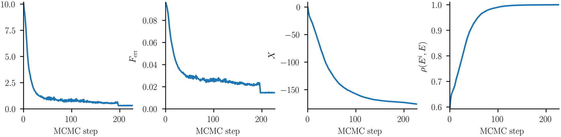
Comparison of parameter convergence diagnostics, as a function of MCMC step for the kinase model inference. This inference was done in two stages: First, a smaller synthetic MSA of size N = 217 ~ 1 × 10⁵ was used until MCMC step 192, after which N was increased to 219 ~ 5 × 10⁵. ℓ1 regularization was used with a strength of λ = 0.00025. (A) The SSR. This levels off to a value of ~ 0.6 until we increase the synthetic MSA size where it lowers to 0.3. (B) Ferr (C) The covariance energy X. This continues to decrease even after the bivariate diagnostics from panels A and B have leveled off. (D) Dataset energy correlations ρ(Ei, E) (see text), which level off suggesting parameter convergence.
Another convergence diagnostic which depends on the sequence energies rather than the bivariate marginals involves the statistical energies of the sequences in the dataset MSA. If the inference has converged, then the relative statistical energies of the sequences in the MSA should not change significantly upon further updates to the couplings. We measure this by the correlation ρ(Ei, E) between the dataset MSA energies E computed with the final coupling values and those computed with couplings from previous iterations Ei, a computation which is insensitive to constant shifts in energy due to gauge transformations. These are shown in Fig. 6C, showing that our model converges to consistent predictions of sequence energy, and that this correlation continues to change even when the bivariate marginals appear to have converged.
The inference is complete once parameter convergence is determined using these diagnostics, and the Potts couplings can be then used in various applications, including contact prediction, prediction of mutant fitness effects, and more. In Fig. 6 we show different measures of parameter convergence for our L = 232, q = 21 kinase model. The rate of parameter convergence depends on model parameters L, q, N and other statistical properties of the data which depend on the protein family being fit as described in Ref [27].
6. Error analysis and Preprocessing tools
In the description of the inference procedure above we took the dataset MSA bivariate marginals as given, without specifying how they were determined. While the inference procedure can be applied to bivariate marginals obtained from arbitrary sources, specific types of preprocessing may be necessary for different types of data and to account for different forms of statistical error. Mi3-GPU includes helper tools for preprocessing of protein-family data for use in protein covariation analysis in particular, to account for biases and statistical error in the sequence data. Some preprocessing steps may only be applicable to certain types of sequence data, for instance the phylogenetic corrections described below may be needed in analysis of “ancient” protein families, but are often not used for single-species viral datasets. For this reason, Mi3 implements such functionality as a set of optional helper scripts. The helper scripts include methods to compute MSA statistics including bivariate marginals with sequence weights accounting for phylogenetic structure, and to compute pseudocounts to account for finite sampling error.
6.1. Sequence Weighting and Histogramming
For inference we assume that the sequences in the MSA are independently generated by the evolutionary process, but this assumption is violated for certain types of datasets, for instance protein-family MSA datasets catalogued in the Pfam database which have phylogenetic relationships. A popular method to account for phylogeny by downweighting similar (likely related) sequences in the dataset was introduced in the earliest Potts-covariation analysis implementations, for instance in Ref. [8]. For each sequence in the dataset one computes the number of other sequences nS with sequence identity above a given threshold θident, which is commonly taken as 20% to 40% of the sequence length. That sequence’s weight is then wS = 1/nS, and one interprets Neff = ∑S wS as the “effective” number of sequences in the dataset. This strategy is used by most covariation analyses of protein-families.
A naive implementation of such pairwise Hamming distance computations requires residue comparisons for N sequences with sequence length L, which in practice can take longer than the inverse Ising inference itself for large N. As an optimization, we note that one can arrange the evaluation order such that after computing all distances to a sequence S one computes distances to the sequence S′ most similar to S. Then the sequence identities for S′ to the MSA can be computed by updating those for S based only on the positions which differ between S and S′. This reduces the number of residue comparisons to where I depends on the range of sequence identities of sequences in the MSA. For our kinase dataset this gives a speedup of 7.7x. We provide scripts using this method to more efficiently compute sequence weights, pairwise sequence similarity histograms and mean sequence identities for an MSA.
6.2. Pseudocounts and Regularization
Finite sampling error is a fundamental source of error or bias in inverse Ising inference, as in other inference problems, and is the cause of overfitting [15, 30, 27]. It arises in inverse Ising inference when estimating bivariate marginals from finite samples of sequences of size N, as described above. Finite sampling causes two different problems we distinguish here: 1. Unsampled residue types (the small-sample case), and 2. Overfitting of the training MSA sequence energies. We address these two problems using regularization and with pseudocounts.
6.3. Covariation-Preserving Pseudocount
The first problem of unsampled or poorly sampled residues types or characters (low counts) causes the relative statistical error to become very large or formally infinite for the corresponding couplings, since the relative binomial sample variance (1 − f)/Nf diverges for small f. This causes division-by-zero errors when evaluating Eq. 2 and unrealistically makes the model predict that such residues are never observed or generated. Similar small-sample problems arises in many statistical contexts, and are commonly accounted for using pseudocounts.
Here we motivate a particular form of pseudocount suited for covariation analysis. The main advantage of this method is that it does not introduce spurious covariances into the data where none were present before pseudocounting, as happens with simpler pseudocount methods, and that it has a Bayesian interpretation. Avoiding spurious correlations is particularly important in protein covariation analysis as detecting the presence or absence of covariance is one of the main goals.
This pseudocount is derived as follows. Consider creating a modified sequence dataset composed of the original sequences but with a small per-position chance μ of mutating to a random residue at each position. For each pair of positions, the probability of mutating both positions is μ2, of mutating only the first position μ(1 − μ), and of no mutation is (1 − μ)2, and so the modified bivariate marginals, which we will use as our pseudocounted marginals, are
| (14) |
and by summing over β the pseudocounted univariate marginals are
| (15) |
This pseudocount uniformly scales down the pairwise covariances as we obtain , where, and so it preserves the relative strength of all covariances, and any pairs whose covariance was previously 0 remains 0.
We choose the pseudocount parameter μ based on a Bayesian analysis of the univariate marginals. Eq. 15 can be rewritten as where N is the sample size, is the sample count for residue i, α, and p is a pseudocount, using the transformation μ = qp/(N +qp). This is the formula used to apply a flat pseudocount p to all the univariate counts and renormalize so the marginals sum to 1. It is also the expected value of the conjugate prior distribution of the multinomial distribution (the Dirichlet distribution) resulting from N Bernoulli trials with p “pseudo-observations”, which models the finite-sampling procedure which produced the MSA. In Bayesian analysis, different choices of p correspond to well-known prior distributions on the marginals, for instance p = 1 is known as the “Bayes” prior and p = 0.5 is a “Jeffrey’s” prior. Choosing one of these priors with corresponding μ, Eq. 14 yields a set of pseudocounted bivariate marginals whose univariate marginals are statistically consistent with the MSA and Bayesian prior, and which also preserve the covariance structure of the MSA.
We contrast this method with that of adding a small flat pseudocount (e.g. of 1/N) to the bivariate marginals, which is equivalent to adding a small number of completely random sequences to the original sequence dataset. Such a flat pseudocount will modify the relative strength of covariances in the MSA among different residues and positions and can introduce covariances where there were none before. In Fig. 7 we compare how different pseudocount strategies help correct for finite sampling error in marginals estimated from a small sample of 1000 sequences from out Potts model, compared to “exact” or reference marginals estimated from a sample of 4 × 10⁶ sequences with very low sampling error. When no pseudocount is used (left panel), 62% of the estimated marginals are measured to be exactly 0, or never observed. When using either a flat pseudocount or our covariant pseudocount, these marginals now have a small but nonzero value, which helps fix issues with 0 observed counts. Furthermore, the pseudocount of Eq. 14 more accurately estimates the value of small bivariate marginals in the lower left area of the plot (right panel).
Figure 7:
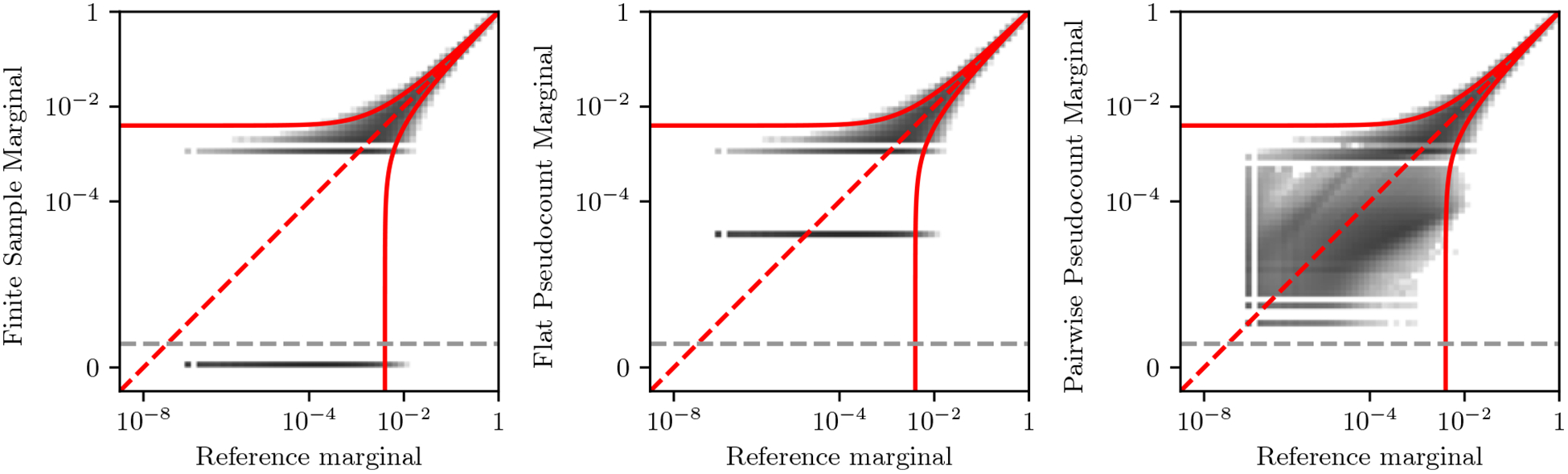
Comparison of pseudocounting strategies to estimate bivariate marginals from a small sample of 1000 sequences, compared to the “exact” or true value of the marginal. Histogram bins are colored according to the logarithm of the bin count. Left: Marginals computed without pseudocounts. Middle: Marginals computed using a flat pseudocount of 0.5/qN, which also function as a Jeffrey’s prior on the univariate marginals. Right: Marginals computed using the covariant pseudocount of Eq. 14 with p = 0.5 which also function as a Jeffrey’s prior on the univariate marginals, showing ability to reconstruct bivariate marginals corresponding to unsampled residue-pairs. In all panels, the Wilson score interval is shown in red for 2 standard deviations to illustrate the magnitude of finite-sampling error for 1000 sequences. Marginals corresponding to 0 counts are show below the dotted gray line.
6.4. Regularization
The other finite-sampling problem is due to ill-conditioning of the inverse Ising problem and to overfitting of the sequence likelihoods P(S) of sequences in the dataset MSA. This problem can occur even if there are no “small sample” problems as described above, and arises due to the collective effect of statistical biases in each model parameter.
Finite sampling and overfitting occur when the dataset MSA has too few sequences, and in Ref. [27] we found that the magnitude of this effect can be measured by a parameter called the “signal-to-noise” ratio (SNR) which can be approximated as SNR ~ Nχ2/θ, where θ is the number of model parameters as described above, which depends on the sequence length L, alphabet size q, dataset MSA depth (number of sequences) N, and a measure of sequence conservation χ. This value may be large (meaning little overfitting) even if the number of sequences N is much smaller than the number of model parameters θ.
Finite sampling error and overfitting can be corrected by various strategies collectively called “regularization”. Often the choice of regularization strategy depends on prior beliefs about the structure of the data, for example some forms of regularization should be used if the interactions are expected to be “sparse” [15]. A common regularization strategy is to add ℓ1 or ℓ2 regularization terms on the coupling parameters to the loss function implicitly used in our derivation above, which is P(S) and which is minimized when the constraint equation is zero as . Our software implements both of these regularization strategies as options by either adding an ℓ1 term or an ℓ2 term to the likelihood. These regularization terms are gauge-dependent, and our software implements them in the “zero-mean” gauge which satisfies as in previous publications [10, 16, 39].
Here we also summarize a different regularization strategy which we have previously developed [27], which is to add a regularization term R = ∑ij γijXij to the loss function, for regularization strengths γij which may differ for each position-pair. This strategy has the advantage that it is gauge-independent, and we can tune it to match the expected statistical error in our datasets due to finite sampling. This strategy can be shown to be equivalent to performing MCMC inference using biased bivariate marginals as , where refers to the marginals sampled from the MSA, to the biased marginals, and to the marginals of the Potts model. Varying γij from 0 to 1 interpolates between the MSA bivariate marginals and the corresponding site-independent bivariate marginals. This bias, which behaves effectively like a pseudocount proportional to the univariate marginals, preserves the univariate marginal constraints while weakening potentially spurious correlations caused by finite sampling error since becomes 0 when γij = 1, and can be implemented as a preprocessing step without needing to modify the MCMC algorithm.
We choose γij such that the discrepancy between the observed marginal and biased marginal is equal to that expected due to sampling error, if one were to take a sample of size N from the biased marginals. That is, based on the discrepancy between the observed marginals and the biased marginals , measured using the “Kullback-Leibler” (KL) divergence . We choose the highest value γij such that the expected discrepancy , where Fαβ are sample marginals drawn from a multinomial distribution around with sample size N. This inequality can be solved numerically for γij by various means, as discussed in Ref. [27]. This should produce a regularized model which has statistical consistency with the observed MSA.
6.5. Conclusions
We have presented a GPU-optimized method for solving the inverse Ising problem using Markov-Chain Monte-Carlo with focus on its application to protein-covariation analysis. The method involves two components: First, a parallel MCMC simulation on the GPU to generate synthetic MSAs given a set of trial Potts Hamiltonian parameters , and second, a parameter-update method accelerated using Zwanzig reweighting techniques. The implementation of the MCMC on the GPU gives a large speedup of 247x compared to a multicore CPU for the GPU and CPU we tested, for datasets most similar to those examined in practice such as protein families catalogued in the Pfam database. Using Zwanzig reweighting techniques, we accelerate parameter convergence by allowing large numbers of coupling updates to be performed for each round of MCMC sequence generations. We developed diagnostics to detect the convergence of the MCMC phase of the inference, as well as convergence of the model parameters to the solution of the inverse Ising problem as the algorithm is iterated. We also provide helper scripts for preparing datasets for use in protein covariation analysis. While our method is designed to model of protein family datasets for which enhanced-sampling techniques appear to be generally unnecessary, the software could be improved in the future to use techniques such as parallel tempering to allow inference in more challenging parameter regimes or types of datasets where these are necessary.
7. Acknowledgements
This work has been supported by grants from the National Institutes of Health (U54-GM103368, R35-GM132090), National Science Foundation (193484), and includes calculations carried out on Temple University’s HPC resources supported in part by the National Science Foundation (1625061) and by the US Army Research Laboratory (W911NF-16-2-0189).
Footnotes
Publisher's Disclaimer: This is a PDF file of an unedited manuscript that has been accepted for publication. As a service to our customers we are providing this early version of the manuscript. The manuscript will undergo copyediting, typesetting, and review of the resulting proof before it is published in its final form. Please note that during the production process errors may be discovered which could affect the content, and all legal disclaimers that apply to the journal pertain.
Declaration of interests
The authors declare that they have no known competing financial interests or personal relationships that could have appeared to influence the work reported in this paper.
References
- [1].Levy RM, Haldane A, Flynn WF, Potts hamiltonian models of protein co-variation, free energy landscapes, and evolutionary fitness, Current Opinion in Structural Biology 43 (2017) 55–62. [DOI] [PMC free article] [PubMed] [Google Scholar]
- [2].Lapedes AS, Giraud B, Liu L, Stormo GD, Seillier-Moiseiwitsch F, Correlated mutations in models of protein sequences: phylogenetic and structural effects, Statistics in molecular biology and genetics Volume 33 (1999) 236–256. [Google Scholar]
- [3].Cocco S, Feinauer C, Figliuzzi M, Monasson R, Weigt M, Inverse statistical physics of protein sequences: a key issues review, Reports on Progress in Physics 81 (2018) 032601. [DOI] [PubMed] [Google Scholar]
- [4].Stein RR, Marks DS, Sander C, Inferring pairwise interactions from biological data using maximum-entropy probability models, PLoS Comput Biol 11 (2015) e1004182. [DOI] [PMC free article] [PubMed] [Google Scholar]
- [5].de Juan D, Pazos F, Valencia A, Emerging methods in protein co-evolution, Nat Rev Genet 14 (2013) 249–261. [DOI] [PubMed] [Google Scholar]
- [6].Serohijos AW, Shakhnovich EI, Merging molecular mechanism and evolution: theory and computation at the interface of biophysics and evolutionary population genetics, Current Opinion in Structural Biology 26 (2014) 84–91. [DOI] [PMC free article] [PubMed] [Google Scholar]
- [7].Mzard M, Mora T, Constraint satisfaction problems and neural networks: A statistical physics perspective, Journal of Physiology-Paris 103 (2009) 107–113. [DOI] [PubMed] [Google Scholar]
- [8].Weigt M, White RA, Szurmant H, Hoch JA, Hwa T, Identification of direct residue contacts in proteinprotein interaction by message passing, PNAS 106 (2009) 67–72. [DOI] [PMC free article] [PubMed] [Google Scholar]
- [9].Sukowska JI, Morcos F, Weigt M, Hwa T, Onuchic JN, Genomics-aided structure prediction, Proceedings of the National Academy of Sciences 109 (2012) 10340–10345. [DOI] [PMC free article] [PubMed] [Google Scholar]
- [10].Ekeberg M, Lvkvist C, Lan Y, Weigt M, Aurell E, Improved contact prediction in proteins: Using pseudolikelihoods to infer potts models, PRE 87 (2013) 012707. [DOI] [PubMed] [Google Scholar]
- [11].Ovchinnikov S, Kinch L, Park H, Liao Y, Pei J, Kim DE, Kamisetty H, Grishin NV, Baker D, Shan Y, Large-scale determination of previously unsolved protein structures using evolutionary information, eLife 4 (2015) e09248. [DOI] [PMC free article] [PubMed] [Google Scholar]
- [12].Pollock DD, Taylor WR, Effectiveness of correlation analysis in identifying protein residues undergoing correlated evolution., Protein Engineering 10 (1997) 647–657. [DOI] [PubMed] [Google Scholar]
- [13].Weigt M, White RA, Szurmant H, Hoch JA, Hwa T, Identification of direct residue contacts in proteinprotein interaction by message passing, Proceedings of the National Academy of Sciences 106 (2009) 67–72. [DOI] [PMC free article] [PubMed] [Google Scholar]
- [14].Morcos F, Pagnani A, Lunt B, Bertolino A, Marks DS, Sander C, Zecchina R, Onuchic JN, Hwa T, Weigt M, Direct-coupling analysis of residue coevolution captures native contacts across many protein families, Proceedings of the National Academy of Sciences 108 (2011) E1293–E1301. [DOI] [PMC free article] [PubMed] [Google Scholar]
- [15].Cocco S, Monasson R, Adaptive cluster expansion for the inverse ising problem: Convergence, algorithm and tests, J Stat Phys 147 (2012) 252–314. [Google Scholar]
- [16].Barton JP, Leonardis ED, Coucke A, Cocco S, Ace: adaptive cluster expansion for maximum entropy graphical model inference, Bioinformatics 32 (2016) 3089–3097. [DOI] [PubMed] [Google Scholar]
- [17].Jacquin H, Gilson A, Shakhnovich E, Cocco S, Monasson R, Benchmarking inverse statistical approaches for protein structure and design with exactly solvable models, PLoS Comput Biol 12 (2016) e1004889. [DOI] [PMC free article] [PubMed] [Google Scholar]
- [18].Sutto L, Marsili S, Valencia A, Gervasio FL, From residue coevolution to protein conformational ensembles and functional dynamics, Proceedings of the National Academy of Sciences 112 (2015) 13567–13572. [DOI] [PMC free article] [PubMed] [Google Scholar]
- [19].Mora T, Bialek W, Are biological systems poised at criticality?, J Stat Phys 144 (2011) 268–302. [Google Scholar]
- [20].Ferguson A, Mann J, Omarjee S, Ndungu T, Walker B, Chakraborty A, Translating hiv sequences into quantitative fitness landscapes predicts viral vulnerabilities for rational immunogen design, Immunity 38 (2013) 606–617. [DOI] [PMC free article] [PubMed] [Google Scholar]
- [21].Zwanzig RW, Hightemperature equation of state by a perturbation method. i. nonpolar gases, J. Chem. Phys 22 (1954) 1420–1426. [Google Scholar]
- [22].Broderick T, Dudik M, Tkacik G, Schapire RE, Bialek W, Faster solutions of the inverse pairwise ising problem, arxiv.org. [Google Scholar]
- [23].Ferrenberg AM, Swendsen RH, New monte carlo technique for studying phase transitions, PRL 61 (1988) 2635–2638. [DOI] [PubMed] [Google Scholar]
- [24].Haldane A, Flynn WF, He P, Vijayan R, Levy RM, Structural propensities of kinase family proteins from a potts model of residue co-variation, Protein Science 25 (2016) 1378–1384. [DOI] [PMC free article] [PubMed] [Google Scholar]
- [25].Haldane A, Flynn WF, He P, Levy RM, Coevolutionary landscape of kinase family proteins: Sequence probabilities and functional motifs, Biophysical Journal 114 (2018) 21–31. [DOI] [PMC free article] [PubMed] [Google Scholar]
- [26].Flynn WF, Haldane A, Torbett BE, Levy RM, Inference of epistatic effects leading to entrenchment and drug resistance in hiv-1 protease, Molecular Biology and Evolution 34 (2017) 1291–1306. [DOI] [PMC free article] [PubMed] [Google Scholar]
- [27].Haldane A, Levy RM, Influence of multiple-sequence-alignment depth on potts statistical models of protein covariation, PRE 99 (2019) 032405. [DOI] [PMC free article] [PubMed] [Google Scholar]
- [28].Henderson GJ, Lee S-K, Irlbeck DM, Harris J, Kline M, Pollom E, Parkin N, Swanstrom R, Interplay between single resistance-associated mutations in the hiv-1 protease and viral infectivity, protease activity, and inhibitor sensitivity, Antimicrob. Agents Chemother 56 (2012) 623. [DOI] [PMC free article] [PubMed] [Google Scholar]
- [29].Biswas A, Haldane A, Arnold E, Levy RM, Wittkopp PJ, Epistasis and entrenchment of drug resistance in hiv-1 subtype b, eLife 8 (2019) e50524. [DOI] [PMC free article] [PubMed] [Google Scholar]
- [30].Cocco S, Monasson R, Adaptive cluster expansion for inferring boltzmann machines with noisy data, PRL 106 (2011) 090601. [DOI] [PubMed] [Google Scholar]
- [31].Cocco S, Monasson R, Weigt M, From principal component to direct coupling analysis of coevolution in proteins: Low-eigenvalue modes are needed for structure prediction, PLoS Comput Biol 9 (2013) e1003176EP. [DOI] [PMC free article] [PubMed] [Google Scholar]
- [32].Tikochinsky Y, Tishby NZ, Levine RD, Alternative approach to maximum-entropy inference, PRA 30 (1984) 2638–2644. [Google Scholar]
- [33].Newman M, Barkema G, Monte carlo methods in statistical physics, Oxford University Press: New York, USA, 1999. [Google Scholar]
- [34].Thomas D, The mwc64x random number generator.(2011), URL: http://cas.ee.ic.ac.uk/people/dt10/research/rngs-gpu-mwc64x.html.
- [35].Cowles MK, Carlin BP, Markov chain monte carlo convergence diagnostics: A comparative review, Journal of the American Statistical Association 91 (1996) 883–904. [Google Scholar]
- [36].Gelman A, Rubin DB, A single series from the gibbs sampler provides a false sense of security, Bayesian statistics 4 (1992) 625–631. [Google Scholar]
- [37].Brooks SP, Roberts GO, Convergence assessment techniques for markov chain monte carlo, Statistics and Computing 8 (1998) 319–335. [Google Scholar]
- [38].Gelman A, Rubin DB, Inference from iterative simulation using multiple sequences, Statist. Sci 7 (1992) 457–472. [Google Scholar]
- [39].Barton JP, Cocco S, Leonardis ED, Monasson R, Large pseudocounts and {L}; {2}-norm penalties are necessary for the mean-field inference of ising and potts models, PRE 90 (2014) 012132–. [DOI] [PubMed] [Google Scholar]