

Abstract
Deep learning has achieved great success in areas such as computer vision and natural language processing. In the past, some work used convolutional networks to process EEG signals and reached or exceeded traditional machine learning methods. We propose a novel network structure and call it QNet. It contains a newly designed attention module: 3D-AM, which is used to learn the attention weights of EEG channels, time points, and feature maps. It provides a way to automatically learn the electrode and time selection. QNet uses a dual branch structure to fuse bilinear vectors for classification. It performs four, three, and two classes on the EEG Motor Movement/Imagery Dataset. The average cross-validation accuracy of 65.82%, 74.75%, and 82.88% was obtained, which are 7.24%, 4.93%, and 2.45% outperforms than the state-of-the-art, respectively. The article also visualizes the attention weights learned by QNet and shows its possible application for electrode channel selection.
Keywords: EEG, Motor imagery, Convolutional neural network, Bilinear vectors, Attention mechanism
Introduction
Motor imagery is one of the ways to realize the brain-computer interface. Another commonly used method is steady-state visual evoked potentials. The advantage of motor imagery is that it can generate control signals without receiving external stimuli, avoiding visually induced eye irritation. However, the accuracy of motor imagery classification is relatively low. Improving the classification accuracy of motor imagery can promote the practical application of brain-computer interface devices based on motor imagery.
The difficulties of the classification task of motor imagery lie in: (1) The measured data contains many artifacts, such as low-frequency drifts, power line noise, heartbeat artifacts (ECG), and ocular artifacts (EOG). The movement of the head during measurement will also bring artifacts. Before classification, manual preprocessing is often required to remove artifacts, which is not conducive to real-time control of BCI systems. (2) Artificial design and feature extraction are required, and a classifier is designed based on this. (3) As people have different capabilities of motor imagery. BCI control does not work for a non-negligible portion of users (about 15% to 30%) Dickhaus et al. (2009). Models learn in one group are not well suited for a new individual. Therefore, to conduct cross-individual cross-validation, high requirements are placed on the generalization ability of the model.
To improve the classification accuracy of motor imagery tasks, a series of methods have been proposed. Traditional methods often need to preprocess the data, remove artifacts, extract features, and design classification algorithms based on features. There are many jobs focused on feature extraction, such as independent component analysis (ICA), which used to extract features for motor imagery classification (Guo and Wu 2010). Principal component analysis (PCA) is used to extract EEG features to distinguish left and right hand motor imagery classification tasks (Vallabhaneni and He 2004). CSP is proposed to extract EEG features (Müller-Gerking et al. 1999). By designing a spatial filter, CSP maximizes the distinguishability of features used by BCI (Ramoser et al. 2000). CSP performance depends on the operational frequency band of the EEG. FBCSP (Kai et al. 2008) is proposed to solve this problem. In the FBCSP method, after the EEG is band-pass filtered to multiple frequency bands, the CSP features are extracted from each of these frequency bands. After the features are extracted, they are mainly classified using linear discriminant analysis (LDA) Belhumeur Peter et al. (2006), random forest (RF) Breiman (2001), and support vector machine (SVM) Chen et al. (2005) as classifiers. These methods still require manual removal of artifacts. The difference is that different features are extracted, and then corresponding classifiers are designed. Problems (1), (2) and (3) remain unsolved.
With the development of deep learning, some deep learning methods have been proposed to deal with motor imagery tasks. Deep learning methods may perform differently in different individuals, some works Li et al. (2018, 2019) and Yan et al. (2018) with respect to stability analysis for neural networks may helpful. The advantage of the deep learning method is that there is no need to manually extract features. The neural network learns end-to-end classifiers through training. EEGNet Lawhern et al. (2018) uses convolutional networks to process EEG signals for classification tasks. A deep ConvNet with a variety of different architectures is proposed in Schirrmeister (2017), which has a better performance than the widely used filter bank commonly used spatial pattern (FBCSP) decoding algorithm. 1-D CNN layers is used to learn temporal and spatial filters for feature extraction (Dose et al. 2018). These methods do not require manual feature acquisition and reached or exceeded traditional machine learning methods. However, in the cross-individual motor imagery classification task, the accuracy rate needs to be improved.
To solve the above problems, we propose an end-to-end convolutional neural network QNet. The original data can be directly inputted to the network through bandpass filtering without manually remove artifacts. Furthermore, convolutional neural networks can automatically extract features through training. We introduced an attention mechanism in three dimensions and designed a 3D-attention module to make the network automatically learn the importance of different electrodes, time points, and feature maps. QNet uses a two-branch structure to learn more features. After fusing the double branches, bilinear vectors are obtained. Finally, the fully connected layer is used as a classifier. The contributions of this paper are as follows:
A new attention module called 3D-Attention Module (3D-AM) is designed, which is used to learn the attention weight of channels, time points, and feature maps.
An end-to-end two-branch convolutional neural network called QNet is proposed, and a bilinear vector is obtained by merging the two-branch structure for classification.
Visualize the weight information learned by the attention module to explain the knowledge acquired by the convolutional neural network, which provides a learnable electrode and time selection method.
The rest of this paper is organized as follows: Sect. 2 describes the structure of QNet and the mathematical formula of 3D-AM in detail. The data set, implementation details, and experimental results are present in Sect. 3. Section 4 discusses the ablation study of the 3-D attention module. Conclusions are given in the Sect. 5.
Methods
In this section, the classification task of motor imagery based on EEG is first formularized. Then, the architecture of QNet is first illustrated in Fig. 1. Finally, the principle of the 3D-Attention Module is explained in detail.
Fig. 1.

The architecture of QNet. It uses the residual learning module (He et al. 2016) as the basic feature extraction module, and combines the 3D-AM module to introduce the attention mechanism. The Q-shaped structure is used to learn the features under different attentions, and the bilinear vector is used to classification
Problem formulation
EEG data are typically time-series data that measure the voltage at each electrode location. It is important to define the EEG data as follows: N means channel number, T represents the total number of sampling points, so the EEG input data , label , c denotes the total number of categories for classification tasks. All of the samples set is , the corresponding label set is .
The neural network is used to learn a function:
| 1 |
where and denotes the probability to each of the classes. is parameters of neural network.
Loss function is cross entropy, which is illustrated in the following :
| 2 |
where is a indicator variable, If ground truth , then , otherwise . By using back-propagation algorithm (Rumelhart et al. 1986), the parameters are adjusted to minimize the loss function.
Overview of QNet architechture
In this work, a neural network with a Q-shaped structure is proposed and named QNet. This model uses residual block (He et al. 2016) as the basic feature extraction module. ResNet18 pre-trained on ImageNet is used as the initial parameter of the residual block in QNet. The architecture of the residual block is shown in Fig. 2. After the EEG data passes through the convolutional network, a feature map channel dimension is added. Each channel corresponds to a feature map. The number of feature map channels is represented by C. The EEG data are expressed as .
Fig. 2.

The architecture of the residual block. It consists of two convolutional layers, with a batchnorm layer and a relu layer in the middle. The input and the data after the convolution layer are added, then activated by relu layer as the output of the residual block
The 3D-AM module was proposed to introduce attention mechanisms. For more information, please see Sect. 2.3. The Q-shaped structure is used to learn the features under different attentions. Bilinear vectors (Lin et al. 2015) can be used to obtain second-order feature information, and this paper uses this second-order information for classification tasks. The fusion method of bilinear vector is shown in (3) and (4).
| 3 |
where are the outputs of A and B branches, respectively. .
| 4 |
where is a function that transform the input z into a 1-dimensional vector, is bilinear vector.
3D-attention module
After analysis of the motor imagery task and related papers Park et al. (2014), Handiru and Prasad (2016) and Loboda et al. (2014), we made the following two assumptions: (1) The importance of each electrode channel is not the same; (2) During the execution of motor imagery tasks, there is a divergence in execution intensity at different sampling times. Not all 64 electrode channels are related to motor imagery tasks. Irrelevant electrode data may even interfere with the network to obtain valid information. Besides, within 4s of performing the motor imagery task, due to the existence of fatigue, we cannot guarantee that there is a strong motor imagery during the 4s. Therefore, the attention mechanism is introduced to the processing of EEG data in accordance with the characteristics of motor imagery task data.
The 3D-attention module is shown in Fig. 3. By permute in (5), the input data is expanded out of and branches.
| 5 |
where , and . refers to permute operations.
Fig. 3.

The architecture of the 3D-Attention Module. By global average pooling, three attention vectors were generated. Softmax is used to standardize the weights, then the outputs of these three attention vectors are fused to generate the 3D-attention map. Finally, weighted input plus the original input as the output of the 3D-Attention Module. means addition and means element-wise multiplication
The global average pooling is used to aggregate global information into an attentive vector (Ni et al. 2019). Convolution operation can only obtain a local perceptive field while global average pooling operation can obtain a global perceptive field. The global information can supplement the network model with richer information and also be used for weight learning of different feature maps, electrodes or sampling times. Equation (6) shows the mathematical description of the global average pooling.
| 6 |
where refers to the global average pooling. All three branches are pooled into a one-dimensional vector through GAP, with size , , and .
Two convolutional layers are used to learn attention weights, with a batchnorm layer and a relu activation layer. Then the softmax layer is used to standardize the weights.
| 7 |
where denotes convolution, refers to batchnorm, represents ReLU function and denotes softmax function. The softmax layer is described in (8).
| 8 |
Next, expand and permute the three branches to size , we can get . 3D-attention map is calculated in the following way:
| 9 |
where and denotes Hadamard product. As shown in (10), the input data is multiplied with the 3D attention map after convolution to obtain features with an attention mechanism. The original input data is added as the output of the entire module.
| 10 |
Experiments
Dataset
We use EEG Motor Movement/Imagery Dataset to verify the effectiveness of our model. This data set consists of EEG Data from 109 volunteers, which is open-sourcing on Physionet (Goldberger 2000). Volunteers were asked to wear a 64-channel EEG cap (Fig. 4) and measure EEG data using the BCI2000 system (Schalk et al. 2004). Each subject performed two one-minute baseline runs (with eyes open or closed), and three two-minute runs of each of the four tasks: (1) open and close left or right fist; (2) imagine opening and closing left or right fist; (3) open and close both fists or both feet; (4) imagine opening and closing both fists or both feet; The data is sampled at 160Hz, due to some unknown reason, three (number 88, 92 and 100) of the 109 subjects were sampled at 128Hz, and subject 104 have missing data. Remove those nonstandard data, a subset of 105 subjects was used in this paper.
Fig. 4.

64 channel sharbrough
The experiment paradigm is shown in Fig. 5. It shows a cycle of one trial, with 2s of rest time before each trial. The subject was then asked to perform a 4s motor imagery task and finally had a 2s rest time.
Fig. 5.
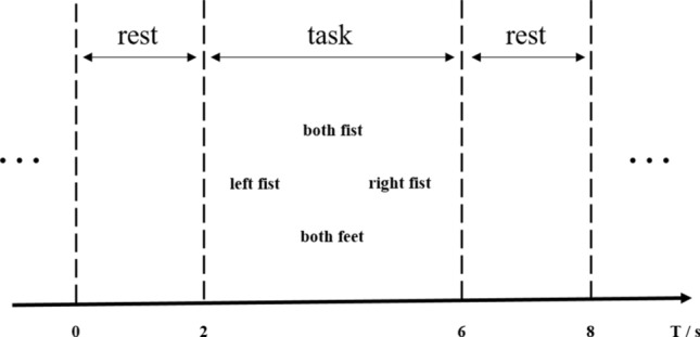
Experiment paradigm. It shows a cycle of one trial, with 2s of rest time before each trial. The subject was then asked to perform a 4s motor imagery task and finally had a 2s rest time
The data of imagine opening and closing left or right fist task was selected to use in this paper. For comparison with Dose (2018), all 64 channels and the first three seconds after the MI task cue data was used to be the input of the network. In this paper, the data set is divided into three subsets, which are used for different classification tasks.
2-class The trails of imagining opening and closing left or right fist. Choose 21 trials for each class, 42 trials per subject in total.
3-class In paper (Dose et al. 2018), a random sections from the baseline recordings with eyes open were used as a third class. The baseline data is about 60s, and 21 trials are randomly selected. So data overlap between different trials is bound to occur. In order to avoid data overlap as much as possible, we intercept the 21 trials at equal intervals to minimize the overlap of samples to compare with this method. The third class refers to the resting state, plus the previous 42 trials, a total of 63 trials per subject.
4-class The fourth class is the simultaneous imagination of both feet. Choose the first 21 trials, plus the previous 63 trials, for a total of 84 trials per subject.
The data we processed has 64 channels. At the same time, during the training, we take the data from 0 to 3s at the beginning of the task. Since the sampling frequency is 160 HZ, there are 481 sample points in total.
Preprocess
EEG data was read through MNE-Python package (Gramfort et al. 2013) and band-pass filtered from 0.1-64 HZ. In order to remove power-line noise, a 60 HZ notch filter was performed. In addition, no other artifacts removal operation is performed. This can verify whether QNet can learn useful information from the data with artifacts.
Implementation details
We used 5 folder cross-validation to evaluate the model. 105 volunteers were divided into 5 groups. Each time, 80% of the subjects (84) were selected for training, and the remaining 20% of the subjects (21) were used as a validation set. Note that this division makes the data of the validation set subjects never participate in training, which is called the global model in Dose et al. (2018). The mean maximum accuracy across all five folders is reported as an accuracy value. In the training process, an early stopping strategy is used. When the verification accuracy of a certain fold does not increase continuously for 20 epochs, the current training is stopped and the next fold training is entered.
Our model is constructed in PyTorch and trained using TITAN Xp GPU. Adam is used as an optimizer. Min-max normalization method is used to normalize the training data to the [0, 1] interval. The normal initialization method is used to initialize the parameters of the convolutional layer. The weights of the batchnorm layer and the fully connected layer are filled with 1, and the bias is set to 0. The batch size is 32. The initial learning rates in the four, three, and two classes of classification tasks are , and , respectively. Set the learning rate of each parameter group using a cosine annealing schedule. In order to prevent the network from overfitting, the weight decay parameters of , and were set. The accuracy history of the 4-class QNet is shown in Fig. 6.
Fig. 6.

4 Class QNet train acc history. The figure shows a history of 5 fold cross-validation accuracy. When each model is trained for about 20 epochs, it can reach about 65% accuracy, which exceeds the state-of-the-art result of 58.58%
Result
The experimental results are shown in Table 1. QNet achieved 65.82%, 74.75%, and 82.88% accuracy in the four, three, and two classes of classification, respectively. To the best of the author knows, the best current result is obtained by Dose et al. (2018). QNet exceeded its 7.24, 4.93, and 2.3 percentage points, respectively, which verified the effectiveness of our model.
Table 1.
Compared with existing methods
| Work | N | Task | Acc (%) | Methods | |
|---|---|---|---|---|---|
| Dose et al. (2018) | 64 | 105 | 4 class | CNN | |
| This work | 64 | 105 | 4 class | QNet | |
| Dose et al. (2018) | 64 | 105 | 3 class | CNN | |
| This work | 64 | 105 | 3 class | QNet | |
| Dose et al. (2018) | 64 | 105 | 2 class | CNN | |
| This work | 64 | 105 | 2 class | QNet | |
| Park et al. (2014) | 58 | 105 | 2 class | SUT-CCSP SVM | |
| Dose et al. (2018) | 58 | 105 | 2 class | CNN | |
| This work | 58 | 105 | 2 class | QNet | |
| Handiru and Prasad (2016) | 16 | 85 | 2 class | FB-CSP SVM classifier | |
| Dose et al. (2018) | 16 | 85 | 2 class | CNN | |
| This work | 16 | 85 | 2 class | QNet | |
| Dose et al. (2018) | 14 | 105 | 2 class | CNN | |
| This work | 14 | 105 | 2 class | QNet | |
| Loboda et al. (2014) | 9 | 103 | 2 class | Phase information | |
| Dose et al. (2018) | 9 | 103 | 2 class | CNN | |
| This work | 9 | 103 | 2 class | QNet |
The bold numbers represent the highest accuracy rate under the same data set and classification task. All accuracy in this table are the results of using 5 fold cross-validation in the EEG Motor Movement/Imagery Dataset. On four, three, and two classification tasks, QNet achieved 65.82%, 74.75%, and 82.88% accuracy, which are 7.24%, 4.93%, and 2.45% outperforms than the state-of-the-art performance. On the same electrode, sample, and classification tasks, QNet is compared with traditional methods in the same dataset. With 16, 58 electrodes, QNet is 10.57%, 15.67% exceed than the traditional method, and 2.62%, 1.26% better than the state-of-the-art. With 14 electrodes, QNet is 2.32% outperforms than the state-of-the-art. In the case of 9 electrodes, QNet is about 5.73% exceed than the traditional method and 1.43% better than the state-of-the-art
To further compare with other methods, QNet is compared with traditional methods that use the EEG Motor Movement/Imagery Dataset. All experiments used the same electrode channels and data as the corresponding papers, and 5 fold cross-validation was used as the final report accuracy rate. With 16, 58 electrodes, QNet is 10.57%, 15.67% exceed than the traditional method, and 2.62%, 1.26% better than the state-of-the-art. With 14 electrodes, QNet is 2.32% outperforms than the state-of-the-art. In the case of 9 electrodes, QNet is about 5.73% exceed than the traditional method and 1.43% better than the state-of-the-art. QNet achieved the best results in all tasks. It is worth noting that both the CNN method in Dose et al. (2018) and the QNet proposed in this paper greatly exceed the results of the traditional method, which may benefit from a large number of samples .
Discussion
Confusion matrix
4 Classification of confusion matrix shown in Fig. 7. The percision of the four categories is 0.735, 0.680, 0.711, and 0.638. The recall rates are 0.712, 0.689, 0.696, and 0.662, respectively. The 63 both class were misclassified into the right class, resulting in a low recall rate of both class; 63 right class and 58 rest state were misclassified as both class, which resulted in a lower precision of both class. It can be seen from the confusion matrix that QNet tends to determine the data as both class, and it is more difficult to distinguish between both class and the right class.
Fig. 7.

4 Class 5 fold confusion matrix. Left, right, rest and both respectively represent imagine opening and closing left fist, imagine opening and closing right fist, resting state and imagine both feet movement. The 63 both class were misclassified into the right class, resulting in a low recall rate of both class; 63 right class and 58 rest state were misclassified as both class, which resulted in a lower precision of both class
Visualization for 3-D attention module
As a novel approach explains the attention learned by 3D-AM, we test the trained model on the validation set. Each sample can get an N-attention vector and a T-attention vector from the first 3D-AM, and the average value is taken as the N vector and T vector. After visualization, the attention head map and temporal attention distribution in Fig. 8 are obtained. The input data of the last two 3D attention modules cannot correspond to the original 64 electrodes, because these data have been down-sampled by the residual block. We only look at the weights gained by the first 3D attention module to get a sense of QNet’s attention.
Fig. 8.

Attention visualization of electrodes and time sampling points extracted from 3D-AM. A, B, and C are the electrode attention visualization results corresponding to the first 3D-attention module classified in four, three, and two classes, respectively; D, E, and F are the corresponding time attention weight maps. In terms of electrodes, if artifacts at the edge of the head topographic map are not considered, the 3D-attention module focuses on the central, frontal, and anterior temporal regions. In terms of time, the main focus is on the 0s-0.8s time period
From the perspective of the electrode’s attention distribution, the edge parts of the head topographic map have larger weights. According to the experience of EEG processing, the edge of the forehead area may correspond to ocular artifacts(EOG), while the edge of the occipital lobe may correspond to abnormal head movements or damaged electrodes. The first 3D-attention module has not been able to eliminate the effects of artifacts well. It should be noted that these results are just the weights learned by the first 3D-attention module. In the next two branches, the two 3D-attention modules will still weight the electrode channels, so the visualization here can only partly represent QNet’s attention. Without considering these artifact components, some interesting phenomena can be observed. In four classification task, the 3D-attention module mainly focuses on the central region C3 and the temporal lobe T8 region; In three classification task, the attention is focused on the central region C3, C2, the frontal region F3, and the anterior temporal lobe region FT7; In two classification task, The classification task focuses on the frontal region F3 and the parietal region P1. Motor cortex is an area of the frontal lobe located in the posterior precentral gyrus immediately anterior to the central sulcus (Donoghue and Sanes 1994), which is basically consistent with the attention area learned by the 3D-attention module.
From the perspective of temporal attention distribution, the attention of all three tasks is concentrated within 0s-0.8s. This may be related to the intensity of motor imagery during the experiment. In the early stages of the instruction, the intensity of motor imagery is the largest. As time increases, the subject may reduce the intensity of motor imagery due to fatigue.
The 3D-attention module provides a way to automatically learn the electrode and time points selection. This may allow us to avoid previous electrode channel selection and directly get a better result. Visualization of attention weights may be used in electrode channel selection of portable brain-computer interface devices.
Conclusion
In this study, we designed QNet, which introduces 3D-AM to learn the attention weights of channels, time pionts, and feature maps. QNet uses a dual branch structure to fuse bilinear vectors for classification. It performs four, three, and two classes on the EEG Motor Movement/Imagery Dataset. The accuracy values of 65.82%, 74.75%, and 82.88% were obtained, which are also the best mean accuracy. This paper also visualizes the attention weights learned by QNet and attempts to explain the results. Deep learning depends on a large number of samples. QNet can achieve excellent performance in the case of a large number of samples, but the effect in the case of a small number of samples needs further verification. The next work will focus on how to transfer the models learned from a large number of samples to a small sample data set to achieve transfer learning between data sets.
Acknowledgements
This work was supported in part by the National Key R&D Program of China (Grant 2018YFC2001700), National Natural Science Foundation of China (Grants 61720106012, U1913601), Beijing Natural Science Foundation (Grant L172050), and by the Strategic Priority Research Program of Chinese Academy of Science (Grant XDB32040000).
Compliance with ethical standards
Conflict of interest
The authors declare that they have no conflict of interest.
Footnotes
Publisher's Note
Springer Nature remains neutral with regard to jurisdictional claims in published maps and institutional affiliations.
Contributor Information
Chen-Chen Fan, Email: fanchenchen2018@ia.ac.cn.
Hongjun Yang, Email: hongjun.yang@ia.ac.cn.
Zeng-Guang Hou, Email: zengguang.hou@ia.ac.cn.
Zhen-Liang Ni, Email: nizhenliang2017@ia.ac.cn.
Sheng Chen, Email: chensheng2016@ia.ac.cn.
Zhijie Fang, Email: fangzhijie2018@ia.ac.cn.
References
- Belhumeur Peter N, Hespanha João P, Kriegman David J (2006) Eigenfaces vs. recognition using class specific linear projection. In: IEEE Computer Society, Fisherfaces
- Breiman L. Random forests. Mach Learn. 2001;45(1):5–32. doi: 10.1023/A:1010933404324. [DOI] [Google Scholar]
- Chen Pai-Hsuen, Lin Chih-Jen, Schölkopf Bernhard. A tutorial on v-support vector machines. Appl Stochast Models Business Ind. 2005;21(2):111–136. doi: 10.1002/asmb.537. [DOI] [Google Scholar]
- Dickhaus T, Sannelli C, Müller KR, Curio G, Blankertz B. Predicting BCI performance to study BCI illiteracy. BMC Neurosci. 2009;10(Suppl 1):1–2. doi: 10.1186/1471-2202-10-S1-P84. [DOI] [Google Scholar]
- Donoghue John P, Sanes Jerome N. Motor areas of the cerebral cortex. J Clin Neurophysiol. 1994;11:4. [PubMed] [Google Scholar]
- Dose H, Møller J, Iversen H, Puthusserypady S (2018) An end-to-end deep learning approach to MI-EEG signal classification for BCIs. Expert Syst Appl 114, 08/01 2018
- Goldberger AL, et al. PhysioBank, PhysioToolkit, and PhysioNet components of a new research resource for complex physiologic signals. Circulation. 2000;101(23):215–220. doi: 10.1161/01.CIR.101.23.e215. [DOI] [PubMed] [Google Scholar]
- Gramfort A et al (2013) MEG and EEG data analysis with MNE-Python (in English). Front Neurosci Methods 7(267), 2013-December-26 [DOI] [PMC free article] [PubMed]
- Guo X, Wu X (2010) Motor imagery EEG classification based on dynamic ICA mixing matrix. In: Proceedings of the 4th international conference on bioinformatics and biomedical engineering (iCBBE ’10), Chengdu, China
- Handiru VS, Prasad VA. Optimized bi-objective EEG channel selection and cross-subject generalization with brain-computer interfaces. IEEE Trans Hum Mach Syst. 2016;46(6):777–786. doi: 10.1109/THMS.2016.2573827. [DOI] [Google Scholar]
- He K, Zhang X, Ren S, Sun J (2016) Identity mappings in deep residual networks. In: European conference on computer vision, pp 630–645
- Kai KA, Zhang YC, Zhang H, Guan C (2008) Filter bank common spatial pattern (FBCSP) in brain-computer interface. In: IEEE international joint conference on neural networks [DOI] [PubMed]
- Lawhern VJ, Solon AJ, Waytowich NR, Gordon SM, Hung CP, Lance BJ. EEGNet: a compact convolutional neural network for EEG-based brain-computer interfaces. J Neural Eng. 2018;15(5):056013. doi: 10.1088/1741-2552/aace8c. [DOI] [PubMed] [Google Scholar]
- Li Z, Bai Y, Huang C, Yan H, Mu S. Improved stability analysis for delayed neural networks. IEEE Trans Neural Netw Learn Syst. 2018;29(9):4535–4541. doi: 10.1109/TNNLS.2017.2743262. [DOI] [PubMed] [Google Scholar]
- Li Z, Yan H, Zhang H, Zhan X, Huang C. Stability analysis for delayed neural networks via improved auxiliary polynomial-based functions. IEEE Trans Neural Netw Learn Syst. 2019;30(8):2562–2568. doi: 10.1109/TNNLS.2018.2877195. [DOI] [PubMed] [Google Scholar]
- Lin T, RoyChowdhury A, Maji S (2015) Bilinear CNN models for fine-grained visual recognition. In: IEEE international conference on computer vision (ICCV), vol 2015, pp 1449–1457
- Loboda A, Margineanu A, Rotariu G, Mihaela A. Discrimination of EEG-based motor imagery tasks by means of a simple phase information method. Int J Adv Res Artif Intell. 2014;3:10. doi: 10.14569/IJARAI.2014.031002. [DOI] [Google Scholar]
- Müller-Gerking J, Pfurtscheller G, Flyvbjerg H. Designing optimal spatial filters for single-trial EEG classification in a movement task. Clin Neurophysiol. 1999;110(5):787–798. doi: 10.1016/S1388-2457(98)00038-8. [DOI] [PubMed] [Google Scholar]
- Ni ZL (2019) RAUNet: Residual Attention U-Net for Semantic Segmentation of Cataract Surgical Instruments. In: Gedeon T., Wong K., Lee M. (eds) Neural Information Processing. ICONIP, et al (2019) Lecture notes in computer science, vol 11954. Springer, Cham
- Park C, Took CC, Mandic DP. Augmented complex common spatial patterns for classification of noncircular EEG from motor imagery tasks. IEEE Trans Neural Syst Rehabil Eng. 2014;22(1):1–10. doi: 10.1109/TNSRE.2013.2294903. [DOI] [PubMed] [Google Scholar]
- Ramoser H, Mullergerking J, Pfurtscheller G. Optimal spatial filtering of single trial EEG during imagined hand movement. Int Conf IEEE Eng Med Biol Soc. 2000;8(4):441–446. doi: 10.1109/86.895946. [DOI] [PubMed] [Google Scholar]
- Rumelhart DE, Hinton GE, Williams RJ. Learning internal representations by error propagation. London: MIT Press; 1986. p. 45. [Google Scholar]
- Schalk G, McFarland DJ, Hinterberger T, Birbaumer N, Wolpaw JR. BCI2000: a general-purpose brain-computer interface (BCI) system. IEEE Trans Biomed Eng. 2004;51(6):1034–1043. doi: 10.1109/TBME.2004.827072. [DOI] [PubMed] [Google Scholar]
- Schirrmeister R et al (2017) Deep learning with convolutional neural networks for EEG decoding and visualization: convolutional Neural Networks in EEG analysis. Human Brain Mapp 38, 08/07 2017 [DOI] [PMC free article] [PubMed]
- Vallabhaneni A, He B. Motor imagery task classification for brain computer interface applications using spatiotemporal principle component analysis. Neurol Res. 2004;26(3):282–287. doi: 10.1179/016164104225013950. [DOI] [PubMed] [Google Scholar]
- Yan H, Zhang H, Yang F, Zhan X, Peng C. Event-triggered asynchronous guaranteed cost control for markov jump discrete-time neural networks with distributed delay and channel fading. IEEE Trans Neural Netw Learn Syst. 2018;29(8):3588–3598. doi: 10.1109/TNNLS.2017.2732240. [DOI] [PubMed] [Google Scholar]