

1. Introduction
Most embryonic mesoderm cells are initially specified when they reside in an epithelium. An epithelial to mesenchymal transition (EMT) then removes them from the epithelial layer and they adapt a mesenchymal phenotype. In some cases, these cells again become epithelial and go through additional EMTs. This process of leaving the epithelium also occurs with carcinoma cells. Whether the two EMTs share mechanistic components of the process is a question that has often been asked. Literature reports indicate that they do indeed share multiple properties: they tend to use the same controlling transcription factors (twist, snail, and zeb1), though not always. They appear similar in behavior (the cells become motile, change polarity, invade through the basement membrane, de-adhere from the adherens junction, and the plasma membrane is remodeled), though differences are observed in different model systems. What is clear is that in both the carcinoma and embryo systems, the molecular basis of this complex cellular event called EMT is incompletely understood. Indeed, of the several thousand papers a year on EMT, most focus on the epiphenomenon, that is, does the phenotypic change occur to an epithelial culture, or layer, under applied experimental conditions? Many fewer papers focus on the functional mechanics of that EMT in molecular detail.
A major reason for not understanding the EMT sequence in greater detail is that most systems are asynchronous, that is, the cells undergoing an EMT are at different states at any given time making it difficult to deduce the precise sequence of molecular events. A few cases of EMT in embryonic systems do offer synchrony, but each of these also has shortcomings. For example ventral furrow formation in Drosophila provides a near synchronous EMT of mesenchyme cells, and some genes necessary for the process have been identified, but the difficulty in that system is that the number of mesenchymal cells is small relative to the remaining cells of the embryo, and the EMT occurs relatively early in development, at a time when many maternally expressed genes are still expressed making it difficult to use the power of Drosophila genetics to discover the genes mechanistically involved specifically in the EMT process (Schafer et. al 2014). Anchor cell invasion in C. elegans is another embryonic model of EMT in which one cell invades through the basement membrane as part of vulval assembly (Schindler et. al 2013). In this case the system is genetically tractable because there is no question of synchrony since only the one cell participates, and a number of genes involved in the process have been identified. The shortcoming of this system for EMT analysis is that the anchor cell does not complete an EMT. It breaches the basement membrane in a manner similar to that utilized by cells undergoing EMT in other systems, but it does not de-adhere from the epithelium. The sea urchin embryo also has a population of cells that undergo EMT at a precise time in early development and a gene regulatory network of specification is well established for those cells, making this a useful model system for understanding control of the process (Saunders et. al 2014). Nevertheless, this system also has shortcomings in that the skeletogenic cells that go through the EMT are only 5% of the population of cells in the embryo, making it a challenge to determine the sequence of molecular events in that small population.
Here we describe a method that can be used on any system to at least partially overcome some of the shortcomings of many systems. Single cell RNA sequencing (scRNA-seq) has advanced to the point where one can obtain a profile of expressed RNA in each cell. Computational approaches along with a temporal trajectory of single cells offers an approach to profile the molecular changes that occur in each cell undergoing the EMT over time. This approach therefore, has the potential of eliminating much of the noise introduced either by asynchrony of the EMT and/or inclusion of non-involved cells, and the reward is provision of a temporal profile of molecular change.
It should be noted, however, that scRNA-seq is not the perfect solution. Because of the small amount of RNA obtained from each cell, amplification is necessary before sequencing. This and other limitations means that some rare RNA species are less likely to be included in the database than in bulk RNA-seq approaches. Nevertheless, the advances in scRNA-seq approaches provide the investigator with a valuable tool to penetrate EMT mechanisms to a level that heretofore has been unreachable.
2. The single cell RNA sequencing approach, a justification.
Next generation sequencing (NGS) platforms increasingly allow in-depth analyses of gene expression and genetic interactions in many biological systems. The approaches allow the investigator unprecedented access to biological questions. The methodology begins with sample preparation, includes library production, sequencing, and data analysis. The latter is most important as software continues to be developed to enable the investigator to gain ever more detail about the biological process in question. As part of the description, the caveats and limitations of these technologies will be discussed. The focus will be on approaches that advance RNA sequencing technologies and their application to Epithelial to Mesenchymal transitions.
Two methods of RNA sequencing are currently utilized, single cell RNA-sequencing (scRNA-seq) and bulk RNA-sequencing (RNA-seq). They each have their own individual advantages and disadvantages and are useful for addressing different biological questions. Bulk (whole-tissue) RNA-sequencing has many applications for research including comparative gene expression analyses between samples of various conditions, differential gene expression, identification of mRNA splice variants and small or long noncoding RNAs. RNA material collected from whole-tissue samples requires less or no amplification relative to sc-RNAseq and the sample can be more deeply sequenced than that obtained from a single cell. Bulk RNA-seq is also easier: obtaining single cell suspensions from fixed or frozen tissue is non-trivial, and may be very difficult for some samples. Thus, bulk-RNA sequencing is a good option in many applications. However, bulk RNA-seq is not as informative for identifying transcriptional differences within heterogeneous cell populations such as in developing and complex tissues because bulk RNA-seq measures the expression level of transcripts across a population of various types of cells, therefore creating an average transcriptomic profile of the tissue. This can become an issue when rare cell types are of interest, because their signal is essentially lost in the noise and more abundant transcripts. One way to get around this issue is by enriching for the population of interest, using a cell surface marker, fluorescence or antibody, however, this will still provide an averaged transcriptome across cells and does not capture heterogeneity at the single cell level. Another way to improve the analysis is to perform a temporal trajectory of the material in question. For embryonic material this can be highly informative because it adds the element of time, although still, within each sample the heterogeneity produces noise.
Single cell RNA sequencing has the potential to eliminate much of the noise within a mixed population of cells. With a temporal profile it enables the investigator to probe the transcriptional dynamics of heterogeneous cell populations because it measures the distribution of mRNA expression from individual cells. Single cell transcriptomes can be profiled for a number of purposes such as creating cell atlases, mapping cell lineage trajectories (Cao et. al 2017, Chen et. al 2018, Fincher et. al 2018, Plass et. al 2018, Tintori et al 2016, Han et. al 2018, Wagner et. al 2018), modeling virtual in situ hybridization (Karaiskos et al 2017) and more (Haque et. al 2017). Using scRNA, one can capture cell trajectories and developmental processes such as an EMT by applying a scRNA-seq time course to construct a cell trajectory map (Griffiths et. al 2018). Generating an EMT time course to capture transient cell states at single cell resolution informs the investigator with information on how this dynamic process occurs over time, providing a resource that is not available in any other known way.
Single cell RNA sequencing is rapidly becoming a viable alternative to bulk RNA sequencing, however, there are still some inherent issues with the platform. One challenge is due to the fact that RNA is harvested from only a single cell, and generally needs to be amplified with reverse transcription or PCR. This process of amplification can introduce bias that can lead to an incorrect interpretation. However, this can be overcome during the normalization and computational analysis by using Unique Molecular Identifiers (UMI), to uniquely label individual RNA molecules, greatly reducing amplification bias. Additionally, due to the sparsity of some RNA transcripts present in the cell and the inefficient cell capture process, sometimes a gene may have moderate expression in some cells, but cannot be detected in another cell. These occurrences, known as gene dropouts can be misleading because it is difficult to differentiate between inefficiency of transcript capture and a cell lacking that particular gene expression, or a gene that is expressed intermittently, therefore dimensionality reduction and normalization should to be performed computationally (Becht et al 2018, Van der Maaten 2008).
3. Preparation of single cell suspensions for scRNA-seq
The key to any scRNA-seq experiment is generating a healthy representative single cell suspension from dissociated tissues or embryos. Therefore, it is imperative to develop a single cell dissociation protocol that properly dissociates all single cells with minimal loss of integrity of the cells and minimal degradation of RNA. To achieve these goals, it is of utmost importance to minimize the time away from a cell’s native environment while generating and handling single cell suspensions to accurately capture a cell’s RNA identity, before alterations can occur. The transient nature of RNA expression can potentially be fixed in time following dissociation with a proper fixative, such as methanol, and the cells washed and rehydrated in 3x SSC rather than PBS, because rehydration in PBS can cause RNA degradation (Juliano et. al 2014, Chen et. al 2018). Tissue types from various organisms and embryos are highly variable in their composition, therefore to generate a single cell suspension, different tissues require different enzymes, temperatures, salinity, and pH. Many groups have utilized enzymes that degrade extracellular matrix components to facilitate their dissociations. To establish a protocol, single cell preparations should be kept consistent, because altering the method of preparation can introduce a sampling bias. To establish the optimal conditions our single cell dissociation protocol was developed using a pilot study to establish the most reliable approach and as part of that, establish that a fixative such as methanol can be used to stabilize the RNA. The pilot study helped establish optimal scRNA-seq conditions for our system. The details of dissociation and stabilization of RNA are too varied to be covered in this chapter, but in each case the goals outlined above should be sought.
4. Considerations of approach and instrumentation available for library preparation from single cells
To a research group beginning a scRNA-seq project, the next big question to ask is what platform should be used? Single Cell RNA sequencing has rapidly evolved since it was first used in 2009 by Tang et. al. When scRNA-seq was first introduced, it involved manually pipetting single cells into microwells and was relatively low throughput with a considerable amount of work required per cell. Since then, many groups have contributed to making scRNA-seq cost efficient and high throughput, and today many variations of these technologies exist. The introduction of multiplexing in 2011 by Islam et. al was a major milestone where they showed many single cells could be sequenced together and quantitatively when UMIs were used. Additionally, in 2013, Brennecke et. al integrated fluidic circuits, to allow for higher throughput, and more reproducibility. In 2015, Macosko et. al and Klein et. al introduced droplet-based methods where single cells are placed in droplets using microfluidics and beads with UMIs to uniquely label RNA molecules in each cell.
Currently a number of platforms are available to choose among, each with its advantages and disadvantages. Platforms differ from each other by either method of RNA quantification, or by method of cell capture. RNA expression is quantified by measure of either full length cDNAs or by tag-based UMIs. There are three methods of cell capture, microwell-based, microfluidic-based, and droplet-based. With the various options, it may seem difficult to determine which method is best, and the answer is it depends on the question being asked. Ziegenhain et. al (2017) and Svensson et. al (2017) realized this and so to assist you in making an informed decision they compare and contrast the common scRNA-seq techniques’ accuracy, sensitivity, precision, power, and cost efficiency. Based on their findings, Smart-seq2, had the best sensitivity, accuracy, precision and the lowest gene dropout rate, however this approach provides relatively low throughput compared to droplet based methods that are not as sensitive but significantly less costly. Smart-seq2 currently is the best option for increased sequencing depth but for a smaller number of cells, as cost can be quite considerable. If willing to sacrifice some sequencing depth, drop-seq is the most cost efficient of the methods, but requires a tedious multi day protocol to be performed. Labs and sequencing centers also are adapting commercial platforms that include Fluidigm’s C1 microfluidic chip, Wafergen ICELL8, BioRad’s ddSEQ, and perhaps the most popular 10x Genomics Chromium. Other alternatives utilize combinatorial indexing such as sciRNA-seq, while SPLiT-seq utilizes a split and pool method of barcoding cells within wells (Cao et. al 2017, Rosenberg et. al 2018) These allow for higher throughput and cost efficiency than 10x and Drop-seq, however, the sample preparation takes longer, and there is a potential for introduction of sampling bias. In addition, the cell quality reportedly is a bit lower than 10x and Drop-seq. With all these options, it can be difficult to identify which method is best, for your research question. For a process such as EMT which has a temporal component, and for a process that occurs within an in vivo model (in our case, the sea urchin), we sought a method that could process many single cells with the best depth possible. To satisfy such a requirement, 10x Genomics was our choice of platform. Following library construction of single cells via 10x Genomics protocol, cells are sequenced at ~50k reads per cell and using a 150 bp paired end Illumina run. Similarly, other single cell library preparation protocols utilize Illumina’s paired end sequencing but may have different run length of 75, 125, 250bp and more. Depending on the number of cells and the run length, a variety of options will be available using Illumina. For example, using a total of 1 billion PE reads on the NovaSeq 6000 and 150bp PE run, roughly, 20k cells can be sequenced at 50k reads/cell to generate a single cell atlas capturing EMT. Indeed, the multitude of scRNA-seq techniques and methods are rapidly evolving, and as cost of scRNAseq decreases, previous technologies will surely become obsolete. Research groups continue to push the limits and cost efficiency of scRNA-seq with methods like cell hashing that allow for “super loading” of cells, and it will only drive the cost down.
5. Bioinformatic Analysis-Overview of procedure for analysis of results
Once single cell libraries are prepared and samples have been sequenced, the first step in analyzing the data is to create an expression matrix from the raw sequencing output. First, your bcl file should be demutiplexed using bcl2fastq to produce fastq files that can be checked for read quality control. A pipeline should be established early to identify what type of analyses will be performed. Following sequencing, Unique Molecular Identifiers (UMI) should be extracted and reads demultiplexed using UMI-tools, or zUMIs (Smith et. al 2016, Parekh et. al 2018). To perform a quality check on your reads, a common tool used is FastQC (Andrews, S. 2010). Once reads have been checked for quality control, they should be trimmed if a sample has poor base per sequence quality scores below 20, or if any exogenous nucleotides such as adapters were introduced. A few commonly used trimming tools are Trimmomatic, TrimGalore, and Cutadapt (Bolger et. al 2014, Krueger et. al 2012, Martin et. al 2011). Trimmed reads can then be mapped back to a reference genome or transcriptome using a bulk RNA-seq aligner/pseudoaligner such as STAR/Kallisto or your aligner appropriate for your research question (Dobin et. al 2013, Bray et. al 2016). Once reads have been mapped to genes, they are counted on a per gene and per cell basis to generate a single cell gene expression matrix (Andrews et. al 2019, Smith et. al 2016). This matrix has a row for each cell and a column for each gene. The i, j entry encodes the number of molecules of mRNA for gene j in cell i. Therefore, each row encodes the expression profile of a cell as a point in a high-dimensional gene-expression space, where there is a dimension for each gene.
With the expression matrix in hand, we are now ready to begin visualizing, exploring and analyzing the data. We begin by visualizing the high-dimensional single-cell gene expression profiles in two or three dimensions. Some popular tools for visualizing single cell datasets include force layout embedding (FLE), UMAP, and tSNE (Brecht et. al 2018, Van der Maaten et al 2008). Instead of applying these tools directly to the single cell expression data, it can be helpful to first reduce the dimensionality from 20,000 down to ~1000 by selecting variable genes, and then down to ~100 using principal components analysis (PCA) or diffusion maps. This gradual decrease in dimensionality can help extract meaningful signals in the visualization. This visualization results in a set of x, y (and maybe z) coordinates that can be used to plot cells as points in 2 or 3 dimensions. Cells can be colored according to time of collection, batch, or expression of individual genes or gene signatures. The second component of exploratory data analysis involves searching for sets of cells with coherent gene expression programs. There are two main ways to do this. The first is to cluster cells (e.g. using Louvain clustering in diffusion component space). The second is to define cell sets according to expression of gene signatures. A gene signature is a list of genes (10 to 100 genes) related to a specific biological process or cell state (e.g. Epithelial Identity). To define an Epithelial cell state, we could select the top 10% of cells with highest expression of the Epithelial Identity gene signature.
In a time-course experiment, an expression matrix is obtained for each time point. The exploratory analysis described above can be applied to all time-points together in order to learn about general trends in expression over time. But, in order to learn about the different developmental trajectories and gene regulatory networks controlling differentiation, we must perform trajectory analysis.
The first goal of trajectory analysis is to infer ancestor-descendant relationships between pairs of time-points. This is crucial because scRNA-seq kills cells; therefore, we cannot use it to directly measure the change in gene expression of any individual cell over time. Live-cell imaging with fluorescent reporters can address this, but only for a handful of genes at a time. Many algorithms have been proposed to recover trajectories from scRNA-seq data. Waddington-OT is the only algorithm developed to date that is capable of modeling cell growth and development in a scRNA-seq time-course. All other algorithms either cannot incorporate known information about time of collection, or assume that all cells grow at the same rate (and therefore give rise to the same number of descendants). Waddington-OT infers ancestor-descendant relationships between pairs of time-points by leveraging a classical mathematical tool called optimal transport (OT). Intuitively, OT is based on the principle that cells can’t change expression of all genes by large amounts in a short period of time. Therefore, cells are connected to “putative descendants” in a way that minimizes the total net change in expression over time. Each cell is allocated a certain amount of “descendant mass” according to an estimate of its proliferative ability and apoptosis rate (i.e. more proliferative cells are connected to more descendants). These growth rates are initially based on gene signatures of cell cycle and apoptosis, but are ultimately learned from data. The output of this first step of trajectory analysis is a “transport matrix” connecting each pair of time-points. The transport matrix has a row for each cell at time 1 and a column for each cell at time 2. The entries of the matrix indicate the amount of descendant mass each cell from time 1 gives rise to at time 2 (if we hadn’t killed the cells).
After inferring ancestor-descendant relationships, the second goal of trajectory analysis is to infer gene regulatory networks controlling development and differentiation. To do this, Waddington-OT looks for transcription factors that are most predictive of transitions to various cell sets. For example, in iPSC reprogramming which transcription factors are responsible for pushing cells towards the stem cell state? Waddington-OT also allows us to analyze the shared ancestry connecting pairs of cell sets. This allows us to answer -- does this pair of cell sets share a common ancestor near the beginning of the time-course and when does the pair diverge? We can then look for transcription factors that explain the bifurcation.
One common drawback of all these techniques is that spatial information is lost when cells are dissociated into suspension, however, the robust characterization of spatial markers within a tissue and developing embryo make it possible to reconstruct spatial patterning in silico. To reconstruct spatial information from dissociated tissues or embryos, Seurat can be employed to estimate a cell’s likely position within spatial domains of the original tissue or embryo. As software matures and techniques improve in resolution, spatial transcriptomic technologies like Spatial Transcriptomics, Slide-Seq, and Seurat can provide more accurate spatial transcriptomic distributions (Eng et. al 2019, Rodrigues et. al 2019).
An outcome sought from this long list of computational options is a list of genes to be used in follow-up mechanistic studies. The question of how to reduce the size of that list varies with the goals in the system. In the case of the EMT, one approach might be to eliminate RNAs that are constitutively expressed since the EMT is fundamentally a change. Then, the direction of change and its timing can be considered using trajectories of RNAs and clustering programs. To that, data on perturbations, either based on known transcription factor control or perhaps on known drug effects can provide differential expression data that helps narrow the candidate list. Ultimately the goal is to identify candidates that are essential to the EMT and will help the investigator understand how the process works. To that end scRNA-seq provides an excellent tool.
Figure 1:
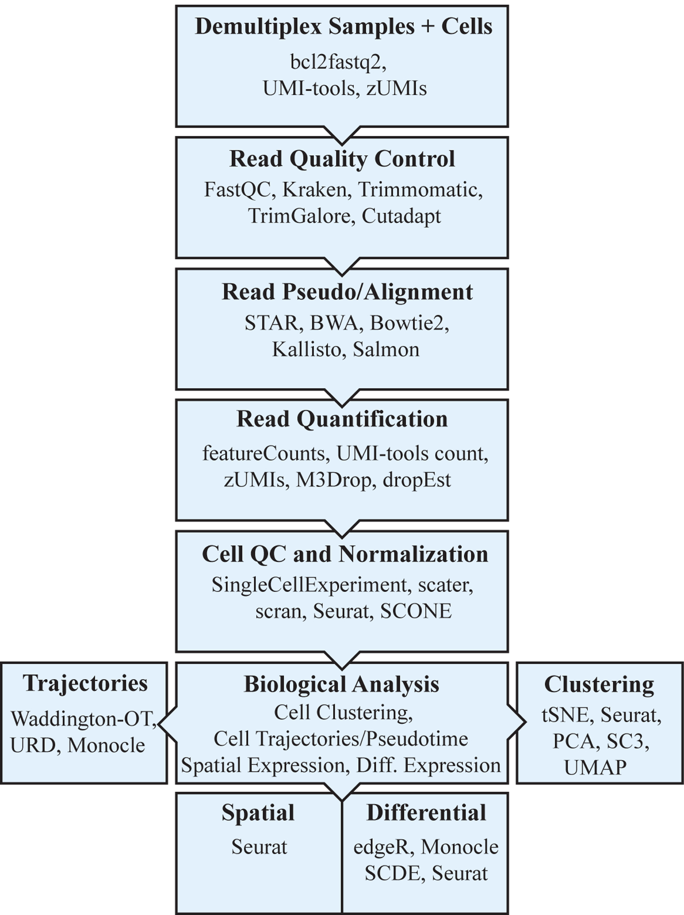
General scRNAseq pipeline
Figure adapted from and inspired by the single cell RNA sequencing course (Kiselev et. al 2019). Bioconductor is a repository that houses toolkits for sequencing and cell quality control, analysis, visualization, exploration, and more. Common packages used for each step in the pipeline are included. Using these methods, each gene’s expression during EMT can be quantitatively measured in single cells, allowing for a deeper understanding of the underlying mechanistic structure of EMT.
Acknowledgements:
The authors thank members of the McClay and the Wray labs for their critical input. We also appreciate the help provided by the Duke Core facility and the Benfey lab in the Biology Department. Support for this project was provided by NIH to DRM (RO1 HD 14483 and PO1 HD037105), and by NSF to GAW (IOS-1457305) and AJM for his NSF predoctoral fellowship (DGE-1644868) and for his NIH predoctoral fellowship (T32-HD040372). GS is supported by a Career Award at the Scientific Interface from the Burroughs Welcome Fund, and by funds from the Klarman Cell Observatory.
Bibliography
- Andrews S, FastQC: a quality control tool for high throughput sequence data. 2010.
- Andrews T (2019). M3Drop: Michaelis-Menten Modelling of Dropouts in single-cell RNASeq. R package version 1.10.0, https://github.com/tallulandrews/M3Drop. [Google Scholar]
- Becht E, et al. “Dimensionality Reduction for Visualizing Single-Cell Data Using Umap.” Nat Biotechnol (2018). Print. [DOI] [PubMed] [Google Scholar]
- Bolger AM, Lohse M, and Usadel B, Trimmomatic: a flexible trimmer for Illumina sequence data. Bioinformatics, 2014. 30(15): p. 2114–20. [DOI] [PMC free article] [PubMed] [Google Scholar]
- Bray NL, et al. “Near-Optimal Probabilistic Rna-Seq Quantification.” Nat Biotechnol 34.5 (2016): 525–7. Print. [DOI] [PubMed] [Google Scholar]
- Brennecke P, et al. “Accounting for Technical Noise in Single-Cell Rna-Seq Experiments.” Nat Methods 10.11 (2013): 1093–5. Print. [DOI] [PubMed] [Google Scholar]
- Cao Junyue, et al. “Comprehensive Single-Cell Transcriptional Profiling of a Multicellular Organism.” Science, vol. 357, no. 6352, 2017, pp. 661–667. [DOI] [PMC free article] [PubMed] [Google Scholar]
- Chen J, et al. “Pbmc Fixation and Processing for Chromium Single-Cell Rna Sequencing.” J Transl Med 16.1 (2018): 198. Print. [DOI] [PMC free article] [PubMed] [Google Scholar]
- Chen J, Renia L, and Ginhoux F, Constructing cell lineages from single-cell transcriptomes. Mol Aspects Med, 2018. 59: p. 95–113. [DOI] [PubMed] [Google Scholar]
- Cole M, Risso D (2019). scone: Single Cell Overview of Normalized Expression data. R package version 1.8.0. [Google Scholar]
- Dobin A, Davis CA, Schlesigner F, Drenkow J, Zaleski C, Jha S, Batut P, Chaisson M, Gingeras TR, STAR: ultrafast universal RNA-seq aligner. Bioinformatics, 2013. 29(1): p. 15–21. [DOI] [PMC free article] [PubMed] [Google Scholar]
- Eng CL, et al. “Transcriptome-Scale Super-Resolved Imaging in Tissues by Rna Seqfish.” Nature 568.7751 (2019): 235–39. Print. [DOI] [PMC free article] [PubMed] [Google Scholar]
- Farrell JA, Wang Y, Riesenfeld SJ, Shekhar K, Regev A, Schier AF, Single-cell reconstruction of developmental trajectories during zebrafish embryogenesis. Science, 2018. 360(6392). [DOI] [PMC free article] [PubMed] [Google Scholar]
- Fincher CT, Wurtzel O, de Hoog T, Kravarik KM, Reddien PW, Cell type transcriptome atlas for the planarian Schmidtea mediterranea. Science, 2018. 360(6391). [DOI] [PMC free article] [PubMed] [Google Scholar]
- Griffiths JA, Scialdone A, and Marioni JC, Using single-cell genomics to understand developmental processes and cell fate decisions. Mol Syst Biol, 2018. 14(4): p. e8046. [DOI] [PMC free article] [PubMed] [Google Scholar]
- Han X, Wang R, Zhou Y, Fei L, Sun H, Lai S, Saadatpour A, Zhou Z, Chen H, Ye F, Huang D, Xu Y, Huang W, Jiang M, Jiang X, Mao J, Chen Y, Lu C, Fang Q, Wang Y, Yue R, Li T, Huang H, Orkin SH, Yuan GC, Chen M, Guo G, Mapping the Mouse Cell Atlas by Microwell-Seq. Cell, 2018. 172(5): p. 1091–1107 e17. [DOI] [PubMed] [Google Scholar]
- Haque A, Engel J, Teichmann SA, Lonnberg T, A practical guide to single-cell RNA sequencing for biomedical research and clinical applications. Genome Med, 2017. 9(1): p. 75. [DOI] [PMC free article] [PubMed] [Google Scholar]
- Islam S, Zeisel A, Joost S, La Manno G, Zajac P, Kasper M, Lonnerberg P, Linnarsson S, Quantitative single-cell RNA-seq with unique molecular identifiers. Nat Methods, 2014. 11(2): p. 163–6. [DOI] [PubMed] [Google Scholar]
- Juliano C, Swartz SZ, Wessel G, Isolating Specific Embryonic Cells of the Sea Urchin by Facs. Methods Mol Biol, 1128, 2014: p.187–96. [DOI] [PMC free article] [PubMed] [Google Scholar]
- Karaiskos Nikos, et al. “The Drosophila Embryo at Single-Cell Transcriptome Resolution.” Science, vol. 358, no. 6360, 2017, pp. 194–199. [DOI] [PubMed] [Google Scholar]
- 62. Kester L and van Oudenaarden A, Single-Cell Transcriptomics Meets Lineage Tracing. Cell Stem Cell, 2018. 23(2): p. 166–179. [DOI] [PubMed] [Google Scholar]
- Kharchenko P, Fan J (2019). scde: Single Cell Differential Expression. R package version 2.12.0, http://pklab.med.harvard.edu/scde. [Google Scholar]
- Kiselev VY, Kirschner K, Schaub MT, Andrews T, Yiu A, Chandra T, Natarajan KN, Reik W, Barahona M, Green AR, Hemberg M (2017). “SC3 - consensus clustering of single-cell RNA-Seq data.” Nature Methods. 10.1038/nmeth.4236. [DOI] [PMC free article] [PubMed] [Google Scholar]
- Kiselev Vladimir, et al. “2 Introduction to Single-Cell RNA-Seq | Analysis of Single Cell RNA-Seq Data.” Seq, 20 May 2019, scrnaseq-course.cog.sanger.ac.uk/website/introduction-to-single-cell-rna-seq.html. [Google Scholar]
- Klein Allon M., Mazutis Linas, Akartuna Ilke, Tallapragada Naren, Veres Adrian, Li Victor, Peshkin Leonid, Weitz David A., and Kirschner Marc W.. 2015. “Droplet Barcoding for Single-Cell Transcriptomics Applied to Embryonic Stem Cells.” Cell 161 (5): 1187–1201. 10.1016/j.cell.2015.04.044. [DOI] [PMC free article] [PubMed] [Google Scholar]
- Krueger F, TrimGalore! [http://www.bioinformatics.babraham.ac.uk/projects/trim_galore/]
- Langmead B, and Salzberg SL. “Fast Gapped-Read Alignment with Bowtie 2.” Nat Methods 9.4 (2012): 357–9. Print. [DOI] [PMC free article] [PubMed] [Google Scholar]
- Li H, and Durbin R. “Fast and Accurate Long-Read Alignment with Burrows-Wheeler Transform.” Bioinformatics 26.5 (2010): 589–95. Print. [DOI] [PMC free article] [PubMed] [Google Scholar]
- Liao Y, Smyth GK, Shi W (2019). “The R package Rsubread is easier, faster, cheaper and better for alignment and quantification of RNA sequencing reads.” Nucleic Acids Research, 20 February, gkz114. doi: 10.1093/nar/gkz114. [DOI] [PMC free article] [PubMed] [Google Scholar]
- Lun A, Risso D (2019). SingleCellExperiment: S4 Classes for Single Cell Data. R package version 1.6.0. [Google Scholar]
- Lun ATL, McCarthy DJ, Marioni JC (2016). “A step-by-step workflow for low-level analysis of single-cell RNA-seq data with Bioconductor.” F1000Res, 5, 2122. doi: 10.12688/f1000research.9501.2. [DOI] [PMC free article] [PubMed] [Google Scholar]
- Macosko Evan Z., Basu Anindita, Satija Rahul, Nemesh James, Shekhar Karthik, Goldman Melissa, Tirosh Itay, et al. 2015. “Highly Parallel Genome-Wide Expression Profiling of Individual Cells Using Nanoliter Droplets.” Cell 161 (5): 1202–14. 10.1016/j.cell.2015.05.002. [DOI] [PMC free article] [PubMed] [Google Scholar]
- Martin M Cutadapt removes adapter sequences from high-throughput sequencing reads. EMBnet J. 2011;17(1):10–12. [Google Scholar]
- McCarthy DJ, Campbell KR, Lun AT, Wills QF Scater: Pre-Processing, Quality Control, Normalization and Visualization of Single-Cell Rna-Seq Data in R. Bioinformatics 33.8 (2017): 1179–86. [DOI] [PMC free article] [PubMed] [Google Scholar]
- Parekh S, et al. “Zumis - a Fast and Flexible Pipeline to Process Rna Sequencing Data with Umis.” Gigascience 7.6 (2018). Print. [DOI] [PMC free article] [PubMed] [Google Scholar]
- Patro R, et al. “Salmon Provides Fast and Bias-Aware Quantification of Transcript Expression.” Nat Methods 14.4 (2017): 417–19. Print. [DOI] [PMC free article] [PubMed] [Google Scholar]
- Petukhov V, et al. “Dropest: Pipeline for Accurate Estimation of Molecular Counts in Droplet-Based Single-Cell Rna-Seq Experiments.” Genome Biol 19.1 (2018): 78. Print. [DOI] [PMC free article] [PubMed] [Google Scholar]
- Picelli Simone, Björklund Åsa K, Faridani Omid R, Sagasser Sven, Winberg Gösta, and Sandberg Rickard. 2013. “Smart-Seq2 for Sensitive Full-Length Transcriptome Profiling in Single Cells.” Nat Meth 10 (11): 1096–8. 10.1038/nmeth.2639. [DOI] [PubMed] [Google Scholar]
- Picelli Simone, Faridani Omid R, Björklund Asa K, Winberg Gösta, Sagasser Sven, and Sandberg Rickard. 2014. “Full-Length RNA-seq from Single Cells Using Smart-Seq2.” Nat. Protoc 9 (1): 171–81. [DOI] [PubMed] [Google Scholar]
- Plass Mireya, et al. “Cell Type Atlas and Lineage Tree of a Whole Complex Animal by Single-Cell Transcriptomics.” Science, vol. 360, no. 6391, May 2018, p. eaaq1723. Crossref, doi: 10.1126/science.aaq1723. [DOI] [PubMed] [Google Scholar]
- Robinson MD, McCarthy DJ, Smyth GK (2010). “edgeR: a Bioconductor package for differential expression analysis of digital gene expression data.” Bioinformatics, 26(1), 139–140. doi: 10.1093/bioinformatics/btp616. [DOI] [PMC free article] [PubMed] [Google Scholar]
- Rodriques SG, et al. “Slide-Seq: A Scalable Technology for Measuring Genome-Wide Expression at High Spatial Resolution.” Science 363.6434 (2019): 1463–67. Print. [DOI] [PMC free article] [PubMed] [Google Scholar]
- Rosenberg AB, Roco CM, Muscat RA, Kuchina A, Sample P, Yao Z, Graybuck LT, Peeler DJ, Mukherjee S, Chen W Pun SH, Sellers DL, Tasic B, Seelig G, Single-cell profiling of the developing mouse brain and spinal cord with split-pool barcoding. Science, 2018. 360(6385): p. 176–182 [DOI] [PMC free article] [PubMed] [Google Scholar]
- Saunders LR, McClay DR, 2014. Sub-circuits of a gene regulatory network control a developmental epithelial-mesenchymal transition. Development 141, 1503–1513. [DOI] [PMC free article] [PubMed] [Google Scholar]
- Satija R, Farrell JA, Gennert D, Schier AF, Regev A, Spatial reconstruction of single cell gene expression data. Nat Biotechnol, 2015. 33(5): p. 495–502. [DOI] [PMC free article] [PubMed] [Google Scholar]
- Schafer G, Narasimha M, Vogelsang E, Leptin M, 2014. Cadherin switching during the formation and differentiation of the Drosophila mesoderm - implications for epithelial-to-mesenchymal transitions. J Cell Sci 127, 1511–1522. [DOI] [PubMed] [Google Scholar]
- Schiebinger G, Shu J, Tabaka M, Cleary B, Subramanian V, Solomon A, Gould J, Liu S, Lin S Berube P, Lee L, Chen J, Brumbaugh J, Rigollet P, Hochedlinger K, Jaenisch R, Regev A, Lander ES, Optimal-Transport Analysis of Single-Cell Gene Expression Identifies Developmental Trajectories in Reprogramming. Cell, 2019. 176(4): p. 928–943 e22. [DOI] [PMC free article] [PubMed] [Google Scholar]
- Schindler AJ, Sherwood DR, 2013. Morphogenesis of the caenorhabditis elegans vulva. Wiley Interdiscip Rev Dev Biol 2, 75–95. [DOI] [PMC free article] [PubMed] [Google Scholar]
- Smith TS, Heger A, and Sudbery I, UMI-tools: Modelling sequencing errors in Unique Molecular Identifiers to improve quantification accuracy. 2016. [DOI] [PMC free article] [PubMed]
- Svensson Valentine, Natarajan Kedar Nath, Ly Lam-Ha, Miragaia Ricardo J, Labalette Charlotte, Macaulay Iain C, Cvejic Ana, and Teichmann Sarah A. 2017. “Power Analysis of Single-Cell RNA-Sequencing Experiments.” Nat Meth 14 (4): 381–87. 10.1038/nmeth.4220. [DOI] [PMC free article] [PubMed] [Google Scholar]
- Tang Fuchou, Barbacioru Catalin, Wang Yangzhou, Nordman Ellen, Lee Clarence, Xu Nanlan, Wang Xiaohui, et al. 2009. “mRNA-Seq Whole-Transcriptome Analysis of a Single Cell.” Nat Meth 6 (5): 377–82. 10.1038/nmeth.1315. [DOI] [PubMed] [Google Scholar]
- Tintori Sophia C., et al. “A Transcriptional Lineage of the Early C. Elegans Embryo.” Developmental Cell, vol. 38, no. 4, August. 2016, pp. 430–44. Crossref, doi: 10.1016/j.devcel.2016.07.025. [DOI] [PMC free article] [PubMed] [Google Scholar]
- Trapnell C, et al. “The Dynamics and Regulators of Cell Fate Decisions Are Revealed by Pseudotemporal Ordering of Single Cells.” Nat Biotechnol 32.4 (2014): 381–86. Print. [DOI] [PMC free article] [PubMed] [Google Scholar]
- Van der Maaten L, and Geoffrey Hinton. “Visualizing Data Using T-SNE.” Journal of Machine Learning Research, vol. 9, no. Nov, 2008, pp. 2579–2605. [Google Scholar]
- Wagner DE, Weinreb C, Collins ZM, Briggs JA, Megason SG, Klein AM, Single cell mapping of gene expression landscapes and lineage in the zebrafish embryo. Science, 2018. 360(6392): p. 981–987. [DOI] [PMC free article] [PubMed] [Google Scholar]
- Wood DE, and Salzberg SL. “Kraken: Ultrafast Metagenomic Sequence Classification Using Exact Alignments.” Genome Biol 15.3 (2014): R46. Print. [DOI] [PMC free article] [PubMed] [Google Scholar]
- Ziegenhain Christoph, Vieth Beate, Parekh Swati, Reinius Björn, Guillaumet-Adkins Amy, Smets Martha, Leonhardt Heinrich, Heyn Holger, Hellmann Ines, and Enard Wolfgang. 2017. “Comparative Analysis of Single-Cell RNA Sequencing Methods.” Molecular Cell 65 (4): 631–643.e4. 10.1016/j.molcel.2017.01.023. [DOI] [PubMed] [Google Scholar]