Speeding up quantum perceptron via shortcuts to adiabaticity

Abstract

The quantum perceptron is a fundamental building block for quantum machine learning. This is a multidisciplinary field that incorporates abilities of quantum computing, such as state superposition and entanglement, to classical machine learning schemes. Motivated by the techniques of shortcuts to adiabaticity, we propose a speed-up quantum perceptron where a control field on the perceptron is inversely engineered leading to a rapid nonlinear response with a sigmoid activation function. This results in faster overall perceptron performance compared to quasi-adiabatic protocols, as well as in enhanced robustness against imperfections in the controls.

Introduction

In the era of information expansion, the merge of quantum information and artificial intelligence will have a transformative impact in science, technology, and our societies^1–3. In particular, classical networks of artificial neurons (or nodes) represent a successful framework for machine learning strategies, with the perceptron being the simplest example of a node⁴. The perceptron is based on the McCulloch-Pitts neuron⁵, and it was originally proposed by Rosenblatt in 1957 to create the first trained networks⁶. Nowadays, extensions of these original ideas such as multilayer perceptrons in networks with interlayer connectivity are exploited to deal with demanding computational tasks.

The emergence of quantum computing and machine learning has boosted the development of both fields^7–13, giving rise to the field of quantum machine learning. In this context, quantum neural networks (QNNs) have attracted growing interest^14,15 since the seminal idea proposed by Kak¹⁶. In particular, the entering of classical machine learning techniques into the quantum domain has the potential to accelerate the performance of different applications such as classification and pattern recognition^2,17–23. In addition, nowadays the excellent degree of quantum control over the registers in modern quantum platforms^24–27 allows the performance of quantum operations with high fidelity, which further feeds the idea of having reliable QNNs. However, the linear and unitary framework of quantum mechanics raises a serious dilemma, since neural networks present nonlinear and dissipative behaviours which are hard to reproduce at the quantum level. To address this challenge, many efforts have been attempted by exploiting quantum measurements^16,28, the quadratic kinetic term to generate nonlinear behaviours²⁹, dissipative¹⁶ or repeat-until-success³⁰ quantum gates, and reversible circuits³¹. Among them, gate-based QNNs³² with training optimization procedures³³ are feasible to implement by a set of unitary operations. Furthermore, gate-based QNNs can behave as variational quantum circuits that encode highly nonlinear transformations while remaining unitary²⁰. Also, a quantum algorithm implementing the quantum version of a binary-valued perceptron was introduced in Ref.¹⁸, showing an exponential advantage in resources storage. Remarkably, a universal quantum perceptron has been proposed as an efficient approximator in Ref.³⁴, where the quantum perceptron is encoded in an Ising model with a sigmoid activation function. In particular, the sigmoid nonlinear response is parametrized by the potential exerted by other neurons, and driven by adiabatic techniques.

In this article, motivated by the nonadiabatic control provided by shortcuts to adiabaticity (STA) techniques^35,36, we design fast sigmoidal responses with the aid of the invariant-based inverse engineering (IE)^37–39. The IE method is based on dynamical modes of Lewis-Riesenfeld invariant instead of one instantaneous eigenstates of the original reference Hamiltonian^40,41. As IE directly imposes boundary conditions in the wave function evolution, the nonlinear activation function of the quantum perceptron encoded in the probability of the excited state can be achieved in a fast and robust way. In particular, an external control field on the perceptron is designed such that it leads to a fast nonlinear activation function with a wide tolerance window to the variation of the input potential induced by neurons in the previous layer. We demonstrate that our method produces solutions that outperform those based on adiabatic techniques, which significantly facilitates the implementation of quantum perceptrons in modern platforms such as nitrogen vacancy (NV) centers in diamond. Note that, the latter are settings where external control fields can be introduced with extraordinary precision⁴².

Results

Quantum perceptron

The capacity of feed-forward neural networks to classify complex data relies in the “universal approximation theorem” proved by Cybenko⁴³, claiming that any continuous function can be written as a linear combination of sigmoid functions. A QNN is also demonstrated as a universal approximator of continuous functions³⁴. In a classical network, a perceptron (or neuron) generates the signal $s_j=f(x_j)$ as a sigmoidal response to the weighted sum of the signals (or outputs) from the neurons in the previous layer. More specifically, $x_j={\sum }_{i=1}^k{w}_{\mathit{ji}}{s}_i-b_j$ with the neuron interconnectivities $w_{\mathit{ji}}$, the bias $b_j$, and $s_i$ being the output of the ith neuron in the previous layer. In analogy with classical neurons, a quantum perceptron can be constructed as a qubit that encodes the nonlinear response to an input potential in the excitation probability, see Fig. 1. One possibility for the latter is the following gate³⁴:

$$\begin{array}{c}\hfill {\widehat{U}}_j({\widehat{x}}_j;f)|0_j⟩=\sqrt{1-f({\widehat{x}}_j)}|0_j⟩+\sqrt{f({\widehat{x}}_j)}|1_j⟩,\end{array}$$ 1

where, in close similarity with the classical case, we have ${\widehat{x}}_j={\sum }_{i=1}^k{w}_{\mathit{ji}}{\widehat{\sigma }}_i^z-b_j$, where ${\widehat{\sigma }}_i^z$ is the z Pauli matrix of the ith neuron (qubit), $w_{\mathit{ji}}$ is interaction between the perceptron j and the ith neuron in the previous layer, $b_j$ is the bias of the perceptron. The transformation in Eq. (1) can be engineered by evolving adiabatically the qubit with the Ising Hamiltonian ($ħ=1$)

$$\begin{array}{cc}\hfill \widehat{H}(t)=& \frac{1}{2}\left[{\widehat{x}}_j,{\widehat{\sigma }}_j^z,+,\mathrm{\Omega },(t),{\widehat{\sigma }}_j^x\right]\hfill \\ \hfill =& \frac{1}{2}\left[\sum _{i=1}^k,(w_{\mathit{ji}}{\widehat{\sigma }}_i^z{\widehat{\sigma }}_j^z),-,b_j,{\widehat{\sigma }}_j^z,+,\mathrm{\Omega },(t),{\widehat{\sigma }}_j^x\right],\hfill \end{array}$$ 2

where the jth qubit (encoding the quantum perceptron) is controlled by an external field $\mathrm{\Omega }(t)$, leading to a tunable energy gap in the dressed-state qubit basis $|\pm ⟩$, with ${\widehat{\sigma }}_j^x|\pm ⟩=\pm |\pm ⟩$. When this perceptron is integrated in a feed-forward neural network, the potential depends on the neurons in earlier layers, as the perceptron interacts with other neurons in the previous layer (labeled by $i=1,\dots ,k$) via the $x_j$ potential, see Fig. 1. Therefore, the network is encoded in a Hilbert space via the external potential exerted by other neurons. The Ising Hamiltonian in Eq. (2) has the reduced eigenstate,

$$\begin{array}{c}\hfill |\mathrm{\Phi }(x_j/\mathrm{\Omega }(t))⟩=\sqrt{1-f(x_j/\mathrm{\Omega }(t))}|0⟩+\sqrt{f(x_j/\mathrm{\Omega }(t))}|1⟩,\end{array}$$ 3

where $x_j$ now represents the lowest eigenvalue of the operator ${\widehat{x}}_j$, while f(x) corresponds to a sigmoid excitation probability

$$\begin{array}{c}\hfill f(x)=\frac{1}{2}\left(1,+,\frac{x}{\sqrt{1+x^2}}\right).\end{array}$$ 4

Figure 1.

Schematic configuration of a quantum perceptron. When it is integrated in a feed-forward neural network, the potential depends on neurons in earlier layers, e.g., ${\widehat{x}}_j={\sum }_{i=1}^k{w}_{\mathit{ji}}{\widehat{\sigma }}_i^z-b_j$, where the activation function of the quantum perceptron is the probability of the excited state $P_j(x_j/{\mathrm{\Omega }}_f)$ at the final time $t=t_f$ in the form of sigmoid-shape, shown in the inset.

In order to generate the state on the right side of Eq. (1), we propose the following strategy: First, a Hadamard gate is applied to drive the state from $|0⟩$ to $|+⟩=(|0⟩+|1⟩)/\sqrt{2}$. Secondly, by appropriately tuning $\mathrm{\Omega }(t)$ according to inverse engineering (IE) techniques (to be explained later), the state $|\mathrm{\Psi }(0)⟩=|+⟩$ evolves to $|\mathrm{\Psi }(t_f)⟩=|\mathrm{\Phi }(x_j/{\mathrm{\Omega }}_f)⟩$ (up to some phase factor that can be eventually canceled by a phase gate), along with one eigenstate of the Lewis-Riesenfeld invariant of $\widehat{H}$, with $|\mathrm{\Phi }(x_j/{\mathrm{\Omega }}_f)⟩$ being the instantaneous eigenstate of $\widehat{H}(t=t_f;{\mathrm{\Omega }}_f)$, and ${\mathrm{\Omega }}_f\equiv \mathrm{\Omega }(t_f)$. It is noteworthy to mention that, unlike the fast quasi-adiabatic passage (FAQUAD) approach³⁴, our method based on IE does not need to achieve the initial condition $\mathrm{\Omega }(0)\gg |x_j|$, as it is not required that the initial state meets one eigenstate of $\widehat{H}(0)$. The latter results in a smooth control field $\mathrm{\Omega }(t)$ which is easy to be used in experiments.

Another possibility to achieve $|\mathrm{\Psi }(t_f)⟩$ from $|\mathrm{\Psi }(0)⟩$ is by an adiabatic driving in a Landau-Zener scheme. However, as it is discussed in Ref.³⁴, this spends long time and may be unfeasible depending on the coherence time of the physical setup that implements the Hamiltonian in Eq. (2).

Accelerating quantum perceptron by IE

We adopt the IE method to achieve the $|\mathrm{\Psi }(0)⟩\to |\mathrm{\Phi }(x_j/{\mathrm{\Omega }}_f)⟩$ state transfer with shorter time than FAQUAD⁴⁴. The control field $\mathrm{\Omega }(t)$ is then engineered to guarantee that at the final evolution time $t=t_f$ the qubit excitation probability $P_j(x_j/{\mathrm{\Omega }}_f)$ corresponds to a sigmoid-like response, i.e. to a mono-valuate f function satisfying $\underset{x\to -\infty }{lim}f(x)\to 0$ and $\underset{x\to \infty }{lim}f(x)\to 1$. Since the universality of neural networks does not rely on the specific shape of the sigmoid function^43,45, e.g. Eq. (4), we quantify the performance of the control field $\mathrm{\Omega }(t)$ in the interval $[-x^{\text{max}},x^{\text{max}}]$ with the distance $C=2-F_0-F_1$. Here $F_0={|⟨0|\mathrm{\Psi }(t_f;x_j/{\mathrm{\Omega }}_f=-x^{\text{max}})⟩|}^2$ and $F_1=|⟨1|\mathrm{\Psi }(t_f;x_j/{\mathrm{\Omega }}_f=x^{\text{max}}){|}^2$ characterize how the engineered states overlap with $|0⟩$ and $|1⟩$, at $x_j/{\mathrm{\Omega }}_f=-x^{\text{max}}$ and $x_j/{\mathrm{\Omega }}_f=x^{\text{max}}$ respectively. Note that, for a sigmoid-like function, $C\to 0$, for $x^{\text{max}}\to \infty$. Meanwhile, in all the numerical results, the activation function is found to be well-behaved, i.e., the function is monotonic and with a sigmoid-like behaviour, $\underset{x\to -\infty }{lim}f(x)\to 0$ and $\underset{x\to \infty }{lim}f(x)\to 1$. As we will see later, our IE technique also provides with robustness with respect to timing errors.

Now we show the procedure to find the control $\mathrm{\Omega }(t)$. To this end, we start with the parameterisation of the dynamical state

$$\begin{array}{c}\hfill |\mathrm{\Psi }(t)⟩=cos(\theta /2)e^{i\beta /2}|0⟩+sin(\theta /2)e^{-i\beta /2}|1⟩,\end{array}$$ 5

with the two unknown polar and azimuthal angles, $\theta \equiv \theta (t)$ and $\beta \equiv \beta (t)$, on the Bloch sphere. Having the state in Eq. (5) at hand, the corresponding orthogonal state $|{\mathrm{\Psi }}_{\perp }(t)⟩$ gets completely determined and the Lewis-Riesenfeld invariant can be thus constructed with constant eigenvalues^37,38. Substituting one of the states ($|\mathrm{\Psi }(t)⟩$ or $|{\mathrm{\Psi }}_{\perp }(t)⟩$) into the time-dependent Schrödinger equation driven by the Hamiltonian in Eq. (2), we obtain the following coupled differential equations (for more details see Methods.)

$$\begin{array}{cc}\hfill \mathrm{\Omega }(t)=& \dot{\theta }/sin\beta ,\hfill \end{array}$$ 6

$$\begin{array}{cc}\hfill x_j=& \dot{\theta }cot\theta cot\beta -\dot{\beta }.\hfill \end{array}$$ 7

Setting the wavefunction $|\mathrm{\Psi }(0)⟩=|+⟩$ and $|\mathrm{\Psi }(t_f)⟩=|\mathrm{\Phi }(x_j/{\mathrm{\Omega }}_f)⟩$ at the initial and final times leads to the boundary conditions

$$\begin{array}{cc}\hfill \theta (0)=& 2{sin}^{-1}\left[\sqrt{f(x_j/\kappa )}\right],\hfill \\ \hfill \theta (t_f)=& 2{sin}^{-1}\left[\sqrt{f(x_j/{\mathrm{\Omega }}_f)}\right],\hfill \end{array}$$ 8

with the introduced $\kappa$ parameter being infinitely large which results in $|\mathrm{\Phi }(x_j/\kappa )⟩=|+⟩$. Also, it is important to remark that $\kappa$ does not need to equal the value of our control $\mathrm{\Omega }(t)$ at $t=0$, as $|\mathrm{\Phi }(x_j/\kappa )⟩$ is not necessarily the eigenstate of $\widehat{H}[t=0;\mathrm{\Omega }(0)]$. In addition, from Eq. (6) one can find the following conditions for the first derivatives of $\theta$ at the boundaries

$$\begin{array}{c}\hfill \dot{\theta }(0)=\mathrm{\Omega }(0)sin\beta (0),\dot{\theta }(t_f)={\mathrm{\Omega }}_{f}sin\beta (t_f).\end{array}$$ 9

We can interpolate $\theta$ by choosing a simple polynomial function $\theta ={\sum }_{i=0}^N{a}_i{t}^i$ and a trigonometric fuction $\theta =a_0+a_{1}t+{\sum }_{i=2}^N{a}_{i}sin[(i-1)\pi t/t_f]$ with less coefficients required for matching the same boundary conditions⁴⁶. The appropriate adoptions on the coefficients can make the solution approach the one gained from optimal control theory⁴⁷. We present the comparison of the performance of activation function by using IE with these two ansatzes and exponential functions inspired by regularized optimal solutions in Supplementary Information. We stress that, unlike the method in Ref.^38,48, in our case $\theta$ and $\beta$ are correlated. We impose $\beta (t_f)=\pi /2$ and $\beta (0)=\pi -ϵ$ (note that we will allow a certain deviation by introducing the $ϵ$ parameter, see later). Once we construct $\theta$, the function $\beta$ can be obtained by solving Eq. (7) with the boundary condition $\beta (t_f)=\pi /2$. After the functions $\theta$ and $\beta$ are obtained, the control field $\mathrm{\Omega }(t)$ is deduced using Eq. (6).

The solution to $\beta$ from Eq. (7) depends on $x_j$ leading to a set of $\mathrm{\Omega }\equiv \mathrm{\Omega }(t,x_j)$. However, in order to make the control independent of the input potential, we set $\mathrm{\Omega }(t)=\mathrm{\Omega }(t,x_j=y)$ where the value of y is chosen such that it minimizes the C distance for different $x_j$ in a certain interval (see next section).

IE performance

As the state evolves from $|\mathrm{\Psi }(0)⟩=|+⟩$, the $\kappa$ parameter should be a large number compared to the input potential $x_j$. We numerically study situations where $\kappa =2000$ and explored the range $|x_j|/{\mathrm{\Omega }}_f\in [-x^{\text{max}},x^{\text{max}}]$, with $x^{\text{max}}=12$. Note that, we consider the situation where $x^{\text{max}}=12$, although our results are not limited to the specific number. We use dimensionless units, by setting the unit of time $t_0$ such that the control field $\mathrm{\Omega }(t)$ is given in terms of $1/t_0$. In addition, we consider an unbiased perceptron with $b_j=0$.

Not limited to a fixed large number of $\kappa$, our method shows the flexibility and the feasibility of the control field. For a case in which we impose ${\mathrm{\Omega }}_f=1$ and solve Eq. (7) with a fixed value for $x_j/{\mathrm{\Omega }}_f=y/{\mathrm{\Omega }}_f=12$, we find $\theta (0)=1.576\simeq \pi /2$. Figure 2a indicates the obtained solutions for $\theta$ and $\beta$ for this case in which we have also selected the operation time $t_f=1$. We find that the boundary condition for $\beta (0)$ is also satisfied with a tiny error of $ϵ=2\times {10}^{-5}$. In this specific case, we find that the designed control $\mathrm{\Omega }(t)$ at $t=0$ is $\mathrm{\Omega }(0)=1999.6\approx \kappa$ when $\kappa =2000$, the initial state corresponds to the eigenstate state of the Hamiltonian. Also, we observed that $\beta (0)$ tends to $\pi$ when $t_f$ gets larger. In Fig. 2b, the control field $\mathrm{\Omega }(t)$ obtained with our method is illustrated. This $\mathrm{\Omega }(t)$ leads to an excitation probability such that it arrives at $P_j(x^{\text{max}})=0.998$. Using the same control field $\mathrm{\Omega }(t)$, we find that the probability of the state $|1⟩$ for other input neural potentials $x_j/{\mathrm{\Omega }}_f\in [-x^{\text{max}},x^{\text{max}}]$ is in the form of a sigmoid-like response ranging from 0 to 1 during the interval, as shown in the inset of Fig. 2b. This proves the successful construction of a sigmoid-shape transfer function, which is a crucial factor for a quantum perceptron. The fields calculated from $\kappa =1000$, $\kappa =500$ lead to the same sigmoid activation function which, as shown in the inset of Fig. 2b, cannot be distinguished to the one derived from $\kappa =2000$.

Figure 2.

(a) The functions of $\theta$ (solid-blue) and $\pi -\beta$ (dashed-red), where $\theta$ is interpolated by a polynomial ansatz $\theta ={\sum }_{i=0}^3{a}_i{t}^i$, and $\beta$ is solved from Eq. (7) for $t_f=1$ and $\kappa =2000$, with $ϵ=2\times {10}^{-5}$. (b) The control fields $\mathrm{\Omega }(t)$ designed from IE (solid-blue) with the help of $\theta$, $\beta$ and from FAQUAD (dashed-red), where $\kappa =2000$. We also show the control fields derived from $\kappa =1000$ (dotted-black) and $\kappa =500$ (dot-dashed-green). The inset in (b) displays the corresponding activation functions for different $\kappa$, which coincide with each other. In both plots, $y/{\mathrm{\Omega }}_f=12$.

Our IE method provides a wider range of $y/{\mathrm{\Omega }}_f$ than FAQUAD to construct sigmoid transfer functions. In Fig. 3a the value of the distance C obtained with the IE method, as a function of $y/{\mathrm{\Omega }}_f$ for various operation times $t_f$, is shown. It can be observed that a low value for C appears with large values for |y| and $t_f$. We have checked (also for $t_f=1$) the appearance of nonlinear perceptron responses that connect 0 and 1 with a sigmoid shape. In particular, these lead to $C<{10}^{-2}$ in the range $y/{\mathrm{\Omega }}_f\in [5,12]$ with control fields $\mathrm{\Omega }(t)$ for $t_f=1$ similar to the one in Fig. 2b. In contrast, C goes to almost 2 at $y/{\mathrm{\Omega }}_f=-x^{\text{max}}$ by FAQUAD techniques⁴⁴, in which only for long $t_f$ and in the regime $y/{\mathrm{\Omega }}_f\to x^{\text{max}}$ the transfer function can be produced, see Fig. 3b.

Figure 3.

The dependence of C value on y with the application of IE $\theta ={\sum }_{i=0}^3{a}_i{t}^i$ (a) and FAQUAD (b) for different operation times $t_f=0.1$ (solid-blue), $t_f=0.2$ (dashed-red), $t_f=0.5$ (dotted-black), and $t_f=1$ (dot-dashed-green).

The target state $|\mathrm{\Psi }(t_f)⟩=|\mathrm{\Phi }(x_j/{\mathrm{\Omega }}_f)⟩$ depends on the value of the driving field at the final time, see Eq. (3). In general we observe that, with our IE method, a larger value of the control field at $t=t_f$ (i.e. ${\mathrm{\Omega }}_f$) offers higher fidelity. As an example of the latter, in Fig. 4 we show the value of C as a function of ${\mathrm{\Omega }}_f$ for $t_f=0.2$ with the application of IE (solid-blue) and FAQUAD (dashed-red). In this figure one can observe the improved performance of our IE method. Actually, every point of the lower value C by IE implies the successful discovery of sigmoid-shape transfer function and driving field $\mathrm{\Omega }(t)$.

Figure 4.

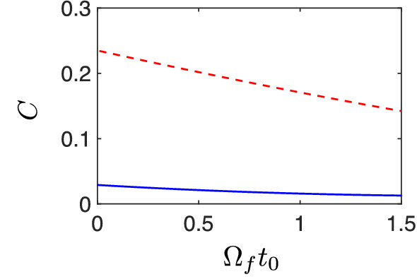
Dependence of C value on ${\mathrm{\Omega }}_f$ is shown for IE $\theta ={\sum }_{i=0}^3{a}_i{t}^i$ (solid-blue) and FAQUAD (red-dashed) protocols, when $t_f=0.2$, $y/{\mathrm{\Omega }}_f=12$.

Quasi-optimal-time solution

As the activation function $P(x_j/{\mathrm{\Omega }}_f)$ connects 0 and 1 at $-x^{\text{max}}$ and $x^{\text{max}}$, we set $C<0.01$ as the criteria of successful construction of a quantum perceptron. In Fig. 5a, we illustrate the dependence of C value on $t_f$ by using the polynomial ansatz $\theta ={\sum }_{i=0}^N{a}_i{t}^i$ with $N=3$ and $N=5$ of IE as well as FAQUAD³⁴. When $N=3$, the smallest $t_f$, such that $C<0.01$ is satisfied, is 0.2, while employing techniques based on FAQUAD, this is at $t_f=0.3$. The further reduction of the smallest $t_f$, such that $C<0.01$ is satisfied, can be improved since IE method allows to approach the quasi-optimal-time solution by introducing more degrees of freedom in the ansatz of $\theta$⁴⁷, leading to faster quantum perceptrons. With $N=5$ (i.e. a solution with two additional parameters, namely $a_4$ and $a_5$), see Fig. 5a (dotted-black curve) we get a speed up of 2 with respect to FAQUAD method, leading to the minimal operation time $t_f^{\text{min}}=0.15$. The values of the transfer function at $-x^{\text{max}}$ and $x^{\text{max}}$ and C value with the application of IE strategies in polynomial, trigonometric and exponential functions as well as FAQUAD can be seen in Supplementary Information, showing that high-order polynomial ansatz can give a quasi-optimal-time solution.

Figure 5.

(a) Dependence of C as a function of the final time $t_f$, using IE in the cases of $\theta ={\sum }_{i=0}^3{a}_i{t}^i$ (solid-blue), $\theta ={\sum }_{i=0}^5{a}_i{t}^i$ (dotted-black) and FAQUAD (dashed-red). The inset of (a) shows the corresponding transfer functions for $t_f=0.15$, where the dotted-black curve represents the quasi-optimal-time solution with $a_2=-50$, $a_3=-3980$. (b) For $t_f=0.15$, the driving field $\mathrm{\Omega }(t)$ designed from IE in the cases of using $\theta ={\sum }_{i=0}^3{a}_i{t}^i$ (solid-blue), using $\theta ={\sum }_{i=0}^5{a}_i{t}^i$ with the optimal parameters $a_2=-50$, $a_3=-3980$ (dotted-black), and $y/{\mathrm{\Omega }}_f=12$.

Moreover, we find that the IE method is robust with respect to timing errors, i.e. variations on the operation time $t_f$. More specifically, once the minimal value of C is reached for solid-blue in Fig. 5a, C does not show any appreciable oscillation for $t>t_f^{\text{min}}$. Conversely, the FAQUAD driving leads to the dashed-red curve in Fig. 5a that shows an oscillatory behavior of C, indicating that only at some specific $t_f$ the sigmoid transfer function can be constructed.

Remarkably, for short times, e.g. $t_f=0.15$, the transfer functions and driving fields are completely different for IE and FAQUAD protocols. In the inset of Fig. 5a,b, we give the detailed demonstration of transfer functions and driving fields designed from IE. On the one hand, FAQUAD protocol cannot produce the sigmoid function, by connecting from 0 to 1 at the edges, see the inset of Fig. 5a dashed-red curve. On the other hand, we find that the case of IE with the polynomial ansatz of $N=3$ fails to connect the state $|0⟩$ presenting $P(-x^{\text{max}})=0.2$ (solid-blue curve). However, We can overcome this limitation by increasing the order of the polynomial ansatz to $N=5$. Here, we compare the activation functions achieved by different strategies at the same value of $y/{\mathrm{\Omega }}_f=12$. It is worth mentioning that by increasing the value of $x^{\text{max}}$ which means more energy is supplied to the system, we can recover a more stretched sigmoid with the FAQUAD protocol or IE with the polynomial ansatz of $N=3$. However, in this work, we find the external driving $\mathrm{\Omega }(t)$ by which the perceptron can have a sigmoidal response in a fixed Hamiltonian configuration with the range $[-x^{\text{max}},x^{\text{max}}]$.

In addition, the derived controls $\mathrm{\Omega }(t)$ from IE methods are smooth and present values close to zero at $t=0$, see Fig. 5b. Compared to the case of $t_f=1$, shorter operation time leads to larger $ϵ$ so that $\mathrm{\Omega }(0)$ is farther away from $\kappa$. This is in contrast with the control $\mathrm{\Omega }(t)$ derived from FAQUAD techniques that demands an abrupt change from $\mathrm{\Omega }(0)=2000$ to $\mathrm{\Omega }(t_f)=1$, see Fig. 2b. This demonstrates the appropriateness of our IE derived controls to be implemented experimentally. In this regard, in the next section we give estimations based on state of the art experimental parameters in NV centers in diamond that demonstrates the suitability of an implementation of our method in such quantum platform.

Discussions

We have demonstrated that the enhanced performance of our method using IE techniques leads to sigmoid activation functions within a minimal operation time of $t_f^{\text{min}}=0.15t_0$. If, for instance, one selects $t_0=500$ ns, the maximum value for the control $\mathrm{\Omega }(t)$ amounts to $|{\mathrm{\Omega }}_{\max }|\approx 50$ MHz for the kind of solutions presented in Fig. 5b (see horizontal axis limits in that figure). This permits the application of our controls in modern quantum platforms such as NV centers in diamond that present coherence times much longer than $0.15t_0=0.15\times 500=75$ ns even at room temperature^49,50. In addition, current arbitrary waveform generators allow to change the amplitude of the delivered microwave field (and consequently of the Rabi frequency $\mathrm{\Omega }$) in time-scales significantly smaller than 1ns^42,51. Then, one can easily introduce the controls in Fig. 5b to produce nonlinear sigmoid responses in NV centers. IE is also helpful to achieve the robust control in a specific physical setup^52–54 when one considers the Ising model with unwanted transitions between the target two-level system and other levels. In this manner one could envision a diamond chip with several NVs, each of them with available nearby nuclear spin qubits, as a quantum hardware to construct QNN using IE methods.

Methods

Inverse engineering and derivation of auxiliary differential equations

The quantum perceptron gate evolves a qubit with the general Hamiltonian (Eq. (2)) which has the instantaneous ground state (Eq. (3)) with the basis $|0⟩={(0,1)}^T$ and $|1⟩={(1,0)}^T$ and a sigmoid excitation probability (Eq. (4)). Therefore, we need to control the final state exactly as $|\mathrm{\Psi }(t_f)⟩=|\mathrm{\Phi }(x_j/\mathrm{\Omega }(t_f))⟩$ in the form of Eq. (3). Inverse engineering by parameterizing the Bloch sphere angles $\theta$ and $\beta$ can manipulate the dynamical state evolution in a fast way. After substituting the wave function $|\mathrm{\Psi }(t)⟩$ (Eq. (5)) or the orthogonal state $|{\mathrm{\Psi }}_{\perp }(t)⟩$ into Schrödinger equation, we can obtain two equations

$$\begin{array}{cc}\hfill -i\dot{\theta }sin\frac{\theta }{2}-\dot{\beta }cos\frac{\theta }{2}=& x_{j}cos\frac{\theta }{2}+\mathrm{\Omega }(t)sin\frac{\theta }{2}{e}^{-i\beta },\hfill \end{array}$$ 10

$$\begin{array}{cc}\hfill i\dot{\theta }cos\frac{\theta }{2}+\dot{\beta }sin\frac{\theta }{2}=& -x_{j}sin\frac{\theta }{2}+\mathrm{\Omega }(t)cos\frac{\theta }{2}{e}^{i\beta }.\hfill \end{array}$$ 11

Eq. (10) $\times sin(\theta /2)$ $+$ Eq. (11) $\times cos(\theta /2)$ and Eq. (10) $\times sin(\theta /2)$ − Eq. (11) $\times cos(\theta /2)$, respectively, result in the analytical expressions of $\mathrm{\Omega }(t)$ (Eq. (6)) and $\beta$ (Eq. (7)). Once setting the operation time $t_f$ and the dynamics of the polar angle $\theta$, we can obtain the function $\beta$ by solving Eq. (7) with the boundary condition $\beta (t_f)=\pi /2$. Hence, from Eq. (6), we derive the applied field $\mathrm{\Omega }(t)$.

Fast quasi-adiabatic method

Another protocol to construct a quantum perceptron by controlling the qubit gate is to use FAQUAD strategy^34,44, which can achieve the fast and adiabatic-like procedure. The adiabatic parameter

$$\begin{array}{c}\hfill \mu (t)=ħ\left|\frac{⟨{\varphi }_0(t)|{\partial }_t{\varphi }_1(t)⟩}{E_1(t)-E_0(t)}\right|\end{array}$$ 12

is kept as a constant $\mu (t)=c$ during the whole control process, where the instantaneous eigenstates for the Hamiltonian (Eq. 2) are

$$\begin{array}{c}\hfill |{\varphi }_l{⟩=cos(\alpha /2)|1⟩+(-1)}^{l}sin(\alpha /2)|0⟩\end{array}$$ 13

with the eigenenergies are $E_l=-{(-1)}^lħ\sqrt{{\mathrm{\Omega }}^2+x_j^2}/2$, $\alpha =arccos\left[-,x_j,/,\sqrt{{\mathrm{\Omega }}^2+x_j^2}\right]$ and $l\in \{0,1\}$. In order to construct a universal quantum gate, a single control should not depend on the neuron potential $x_j$. The largest value $|\mu |$ occurs at $|x_j/{\mathrm{\Omega }}_f|\approx 1.272$. We take this $\mu$ value as an optimal condition that works for all input neuron configurations. As the relation between the field and time is invertible, we can apply the chain rule to Eq. (12) and obtain

$$\begin{array}{c}\hfill \frac{d\mathrm{\Omega }}{\mathit{dt}}=-\frac{c}{ħ}\left|\frac{E_1(\mathrm{\Omega })-E_0(\mathrm{\Omega })}{⟨{\varphi }_0(\mathrm{\Omega })|{\partial }_{\mathrm{\Omega }}{\varphi }_1(\mathrm{\Omega })⟩}\right|,\end{array}$$ 14

where the negative sign represents $\mathrm{\Omega }(t)$ monotonously decreases from $\mathrm{\Omega }(0)$ to $\mathrm{\Omega }(t_f)$. The total duration time is rescaled as $s=t/t_f$ so that $\tilde{\mathrm{\Omega }}(s):=\mathrm{\Omega }(s{t}_f)$ and $d\mathrm{\Omega }/dt=t_f^{-1}d\tilde{\mathrm{\Omega }}/ds$. As a result, we have

$$\begin{array}{cc}\hfill \frac{d\tilde{\mathrm{\Omega }}}{\mathit{ds}}=& -\frac{\tilde{c}}{ħ}{\left|\frac{E_1-E_0}{⟨{\varphi }_0|{\partial }_{\tilde{\mathrm{\Omega }}}{\varphi }_1⟩}\right|}_{\tilde{\mathrm{\Omega }}},\hfill \end{array}$$ 15

$$\begin{array}{cc}\hfill \tilde{c}=& c{t}_f=-ħ{\int }_{\tilde{\mathrm{\Omega }}(0)}^{\tilde{\mathrm{\Omega }}(1)}\frac{d\tilde{\mathrm{\Omega }}}{{\left|\frac{E_1-E_0}{⟨{\varphi }_0|{\partial }_{\tilde{\mathrm{\Omega }}}{\varphi }_1⟩}\right|}_{\tilde{\mathrm{\Omega }}}}.\hfill \end{array}$$ 16

A selection of $t_f$ corresponds to different scaling of $\tilde{c}$ and $\mathrm{\Omega }(t=s{t}_f)=\tilde{\mathrm{\Omega }}(s)$. Consequently, we can derive $\mathrm{\Omega }(t)$ from $\tilde{\mathrm{\Omega }}(s)$ by solving the differential equation (Eq. (15)).

Author contributions

Y.B. developed the theoretical formalism, performed the analytic calculations and performed the numerical simulations. X.C. and E.T. verified the analytical method. J.C. supervised the project. All the authors contributed to the final version of the manuscript.

Competing interests

The authors declare no competing interests.

Supplementary Information

The online version contains supplementary material available at 10.1038/s41598-021-85208-3.

References

- 1.Arute F, Arya K, Babbush R, et al. Quantum supremacy using a programmable superconducting processor. Nature. 2019;574:505–510. doi: 10.1038/s41586-019-1666-5. [DOI] [PubMed] [Google Scholar]
- 2.Biamonte J, Wittek P, Pancotti N, Rebentrost P, Wiebe N, Lloyd S. Quantum machine learning. Nature. 2017;549:195–202. doi: 10.1038/nature23474. [DOI] [PubMed] [Google Scholar]
- 3.Schuld M, Sinayskiy I, Petruccione F. An introduction to quantum machine learning. Contemp. Phys. 2015;56:172–185. doi: 10.1080/00107514.2014.964942. [DOI] [Google Scholar]
- 4.Minsky M, Papert S. A. Perceptrons: An Introduction to Computational Geometry Text. Cambridgem: MIT Press; 2017. [Google Scholar]
- 5.McCulloch WS, Pitts W. A logical calculus of the ideas immanent in nervous activities. Bull. Math. Biophys. 1949;5:115. doi: 10.1007/BF02478259. [DOI] [PubMed] [Google Scholar]
- 6.Rosenblatt, F. Tech. Rep. Inc. Report No. 85-460-1 (Cornell Aeronautical Laboratory, 1957).
- 7.Gyongyosi L, Imre S. A survey on quantum computing technology. Comput. Sci. Rev. 2019;31:51–71. doi: 10.1016/j.cosrev.2018.11.002. [DOI] [Google Scholar]
- 8.Gyongyosi L, Imre S, Nguyen HV. A survey on quantum channel capacities. IEEE Commun. Surv. Tutor. 2018;20:2. doi: 10.1109/COMST.2017.2786748. [DOI] [Google Scholar]
- 9.Gyongyosi L. Unsupervised quantum gate control for gate-model quantum computers. Sci. Rep. 2020;10:10701. doi: 10.1038/s41598-020-67018-1. [DOI] [PMC free article] [PubMed] [Google Scholar]
- 10.Gyongyosi L, Imre S. Optimizing high-efficiency quantum memory with quantum machine learning for near-term quantum devices. Sci. Rep. 2020;10:135. doi: 10.1038/s41598-019-56689-0. [DOI] [PMC free article] [PubMed] [Google Scholar]
- 11.Gyongyosi L, Imre S. Circuit depth reduction for gate-model quantum computers. Sci. Rep. 2020;10:11229. doi: 10.1038/s41598-020-67014-5. [DOI] [PMC free article] [PubMed] [Google Scholar]
- 12.Gyongyosi L. Quantum state optimization and computational pathway evaluation for gate-model quantum computers. Sci. Rep. 2020;10:4543. doi: 10.1038/s41598-020-61316-4. [DOI] [PMC free article] [PubMed] [Google Scholar]
- 13.Gyongyosi L, Imre S. Dense quantum measurement theory. Sci. Rep. 2019;9:6755. doi: 10.1038/s41598-019-43250-2. [DOI] [PMC free article] [PubMed] [Google Scholar]
- 14.Schuld M, Sinayskiy I, Petruccione F. The quest for a quantum neural network. Quant. Inf. Process. 2014;13:25672586. doi: 10.1007/s11128-014-0809-8. [DOI] [Google Scholar]
- 15.Ciliberto C, Herbster M, Ialongo AD, Pontil M, Rocchetto A, Severini S, Wossnig L. Quantum machine learning: A classical perspective. Proc. R. Soc. A. 2018;474:20170551. doi: 10.1098/rspa.2017.0551. [DOI] [PMC free article] [PubMed] [Google Scholar]
- 16.Kak S. On quantum neural computing. Inform. Sci. 2015;83:143–160. doi: 10.1016/0020-0255(94)00095-S. [DOI] [Google Scholar]
- 17.Dunjko V, Briegel HJ. Machine learning and artificial intelligence in the quantum domain: A review of recent progress Rep. Prog. Phys. 2018;81:074001. doi: 10.1088/1361-6633/aab406. [DOI] [PubMed] [Google Scholar]
- 18.Tacchino F., Macchiavello C., et al. An artificial neuron implemented on an actual quantum processor. NPJ Quantum Inf. 2019;5:26. doi: 10.1038/s41534-019-0140-4. [DOI] [Google Scholar]
- 19.Ouyang X. L., Huang X. Z. Experimental demonstration of quantum-enhanced machine learning in a nitrogen-vacancy-center system. Phys. Rev. A. 2020;101:012307. doi: 10.1103/PhysRevA.101.012307. [DOI] [Google Scholar]
- 20.Killoran N, Bromley TR, Arrazola JM, Schuld M, Quesada N, Lloyd S. Continuous-variable quantum neural networks. Phys. Rev. Res. 2019;1:033063. doi: 10.1103/PhysRevResearch.1.033063. [DOI] [Google Scholar]
- 21.Rebentrost P, Bromley TR, Weedbrook C, Lloyd S. Quantum Hopfield neural network. Phys. Rev. A. 2018;98:042308. doi: 10.1103/PhysRevA.98.042308. [DOI] [Google Scholar]
- 22.Zhao J, Zhang YH, Shao CP, Wu YC, Guo GC, Guo GP. Building quantum neural networks based on a swap test. Phys. Rev. A. 2019;100:012334. doi: 10.1103/PhysRevA.100.012334. [DOI] [Google Scholar]
- 23.Li Y, Zhou R, Xu R, Luo J, Hu W. Quantum deep convolutional neural network for image recognition. Quantum Sci. Technol. 2020;5:044003. doi: 10.1088/2058-9565/ab9f93. [DOI] [Google Scholar]
- 24.Leibfried D, Blatt R, Monroe C, Wineland D. Quantum dynamics of single trapped ions. Rev. Mod. Phys. 2003;75:281. doi: 10.1103/RevModPhys.75.281. [DOI] [Google Scholar]
- 25.Devoret MH, Schoelkopf RJ. Superconducting circuits for quantum information: An outlook. Science. 2013;339:1169–1174. doi: 10.1126/science.1231930. [DOI] [PubMed] [Google Scholar]
- 26.Bloch I. Ultracold quantum gases in optical lattices. Nat. Phys. 2005;1:23–30. doi: 10.1038/nphys138. [DOI] [Google Scholar]
- 27.O’Brien JL, Furusawa A, Vučković J. Photonic quantum technologies. Nat. Photon. 2009;3:687. doi: 10.1038/nphoton.2009.229. [DOI] [Google Scholar]
- 28.Zak M, Williams CP. Quantum neural nets. Int. J. Theor. Phys. 1998;37:651–684. doi: 10.1023/A:1026656110699. [DOI] [Google Scholar]
- 29.Behrman EC, Nash LR, Steck JE, Chandrashekar VG, Skinner SR. Simulations of quantum neural networks. Inf. Sci. 2000;128:257–269. doi: 10.1016/S0020-0255(00)00056-6. [DOI] [Google Scholar]
- 30.Cao, Y., Guerreschi, G. G. & Aspuru-Guzik, A. Quantum Neuron: An elementary building block for machine learning on quantum computers. arXiv:1711.11240 (2017).
- 31.Wan KH, Dahlsten O, Kristjánsson H, Gardner R, Kim MS. Quantum generalisation of feedforward neural networks. NPJ Quant. Inf. 2017;3:36. doi: 10.1038/s41534-017-0032-4. [DOI] [Google Scholar]
- 32.Farhi, E. & Neven, H. Classification with Quantum Neural Networks on Near Term Processors. arXiv:1802.06002 (2018).
- 33.Gyongyosi L, Imre S. Training optimization for gate-model quantum neural networks. Sci. Rep. 2019;9:12679. doi: 10.1038/s41598-019-48892-w. [DOI] [PMC free article] [PubMed] [Google Scholar]
- 34.Torrontegui E, García-Ripoll JJ. Unitary quantum perceptron as efficient universal approximator. Europhys. Lett. 2019;125:30004. doi: 10.1209/0295-5075/125/30004. [DOI] [Google Scholar]
- 35.Torrontegui E, Ibáñez S, Martínez-Garaot S, Modugno M, del Campo A, Guéry-Odelin D, Ruschhaupt A, Chen X, Muga JG. Shortcuts to adiabaticity. Adv. At. Mol. Opt. Phys. 2013;62:117. doi: 10.1016/B978-0-12-408090-4.00002-5. [DOI] [Google Scholar]
- 36.Guéry-Odelin D, Ruschhaupt A, Kiely A, Torrontegui E, Martínez-Garaot S, Muga JG. Shortcuts to adiabaticity: Concepts, methods, and applications. Rev. Mod. Phys. 2019;91:045001. doi: 10.1103/RevModPhys.91.045001. [DOI] [Google Scholar]
- 37.Chen X, Ruschhaupt A, Schmidt S, del Campo A, Guéry-Odelin D, Muga JG. Fast optimal frictionless atom cooling in harmonic traps: Shortcut to adiabaticity. Phys. Rev. Lett. 2010;104:063002. doi: 10.1103/PhysRevLett.104.063002. [DOI] [PubMed] [Google Scholar]
- 38.Chen X, Torrontegui E, Muga JG. Lewis-Riesenfeld invariants and transitionless quantum driving. Phys. Rev. A. 2011;83:062116. doi: 10.1103/PhysRevA.83.062116. [DOI] [Google Scholar]
- 39.Shen CP, Wu JL, Su SL, Liang E. Construction of robust Rydberg controlled-phase gates. Opt. Lett. 2019;44:2036. doi: 10.1364/OL.44.002036. [DOI] [PubMed] [Google Scholar]
- 40.Berry MV. Transitionless quantum driving. J. Phys. A Math. Theor. 2009;42:365303. doi: 10.1088/1751-8113/42/36/365303. [DOI] [Google Scholar]
- 41.Wu JL, Su SL. Universal speeded-up adiabatic geometric quantum computation in three-level systems via counterdiabatic driving. J. Phys. A Math. Theor. 2019;52:335301. doi: 10.1088/1751-8121/ab2a92. [DOI] [Google Scholar]
- 42.Zopes J, Sasaki K, Cujia KS, Boss JM, Chang K, Segawa TF, Itoh KM, Degen CL. High-resolution quantum sensing with shaped control pulses. Phys. Rev. Lett. 2017;119:260501. doi: 10.1103/PhysRevLett.119.260501. [DOI] [PubMed] [Google Scholar]
- 43.Cybenko G. Approximation by superpositions of a sigmoidal function. Math. Control Signals Syst. 1989;2:303–314. doi: 10.1007/BF02551274. [DOI] [Google Scholar]
- 44.Martínez-Garaot S, Ruschhaupt A, Gillet J, Busch T, Muga JG. Fast quasiadiabatic dynamics. Phys. Rev. A. 2015;92:043406. doi: 10.1103/PhysRevA.92.043406. [DOI] [Google Scholar]
- 45.Hornik K, Stinchcombe M, White H. Multilayer feedforward networks are universal approximators. Neural Netw. 1989;2:359–366. doi: 10.1016/0893-6080(89)90020-8. [DOI] [Google Scholar]
- 46.Biagiotti L, Melchiorri C. Trajectory Planning for Automatic Machines and Robots. Berlin: Springer; 2008. [Google Scholar]
- 47.Martikyan V, Guéry-Odelin D, Sugny D. Comparison between optimal control and shortcut to adiabaticity protocols in a linear control system. Phys. Rev. A. 2020;101:013423. doi: 10.1103/PhysRevA.101.013423. [DOI] [Google Scholar]
- 48.Takahashi K. Shortcuts to adiabaticity for quantum annealing. Phys. Rev. A. 2017;95:012309. doi: 10.1103/PhysRevA.95.012309. [DOI] [Google Scholar]
- 49.Doherty MW, Manson NB, Delaney P, Jelezko F, Wrachtrup J, Hollenberg LCL. The nitrogen-vacancy colour centre in diamond. Phys. Rep. 2013;528:1–46. doi: 10.1016/j.physrep.2013.02.001. [DOI] [Google Scholar]
- 50.Dobrovitski VV, Fuchs GD, Falk AL, Santori C, Awschalom DD. Quantum control over single spins in diamond. Annu. Rev. Condens. Matter Phys. 2013;4:23. doi: 10.1146/annurev-conmatphys-030212-184238. [DOI] [Google Scholar]
- 51.Boris Naydenov, private communication.
- 52.Kiely A, Ruschhaupt A. Inhibiting unwanted transitions in population transfer in two- and three-level quantum systems. J. Phys. B At. Mol. Opt. Phys. 2014;47:115501. doi: 10.1088/0953-4075/47/11/115501. [DOI] [Google Scholar]
- 53.Yu X, Zhang Q, Ban Y, Chen X. Fast and robust control of two interacting spins Phys. Rev. A. 2018;97:062317. doi: 10.1103/PhysRevA.97.062317. [DOI] [Google Scholar]
- 54.Yan Y, Li Y, Kinos A, Walther A, Shi C, Rippe L, Moser J, Kröll S, Chen X. Inverse engineering of shortcut pulses for high fidelity initialization on qubits closely spaced in frequency. Opt. Express. 2019;27:8267–8282. doi: 10.1364/OE.27.008267. [DOI] [PubMed] [Google Scholar]
Associated Data
This section collects any data citations, data availability statements, or supplementary materials included in this article.