On selecting the critical boundary functions in group-sequential trials with two time-to-event outcomes

Abstract

We investigate selection of critical boundary functions for testing the hypotheses of two time-to-event outcomes as both primary endpoints or a primary and a secondary endpoint in group-sequential clinical trials, where (1) the effect sizes of endpoints are unequal, or (2) one endpoint is for short-term evaluation and the other for long-term evaluation. Bonferroni-Holm and fixed-sequence procedures are considered. We assess the effects of the magnitudes of the hazard ratios and the correlation between the endpoints on statistical powers and provide guidance for consideration.

1. Introduction

We investigate combinations of critical boundary functions for testing the hypotheses associated with two time-to-event outcomes as both primary endpoints, or a primary and a secondary endpoint, in group-sequential clinical trials, which can maximize the power of rejecting either or both of the null hypotheses associated with the two endpoints.

Glimm et al. [1] and Tamhane et al. [2] considered a situation where the two endpoints are evaluated using the fixed-sequence procedure in a group-sequential clinical trial with one interim and a final analysis. They assumed that the statistical information fraction for each endpoint is the same at a particular time-point of analysis and the trial is terminated when the null hypothesis of the primary endpoint is rejected regardless of whether the null hypothesis of the secondary endpoint is rejected. They illustrated that the O’Brien-Fleming-type boundary function (OBF) [3] for the primary endpoint and the Pocock-type boundary function (POC) [4] for the secondary endpoint generally gives the best power for rejecting both of the null hypotheses. However, these findings may not always be applicable when testing the hypotheses associated with two time-to-event endpoints. A few example scenarios are given below:

• In practice, many trials may be not terminated even if the null hypothesis of primary endpoint is rejected at an interim analysis. For example, in oncology, the trial often continues to evaluate overall survival (OS) even if the null hypothesis of progression-free survival (PFS) has been rejected given that OS is more important than PFS.

• As Hung et al. [5] noted, in cardiovascular trials with a composite of major adverse cardiac events (MACE) including all-cause death, myocardial infarction and stroke as a primary endpoint, and all-cause death as a secondary, if the trial is not terminated, POC could not maximize the power for all-cause death since it generally requires a larger sample size or longer follow-up duration due to fewer deaths observed than that for MACE. POC spends a substantial portion of significance level (α) in earlier analyses leaving less α for later analyses.

• Unlike continuous and binary endpoints, when using logrank test or proportional hazard regression with alternatives that satisfy the proportional hazard assumption, the amount of statistical information characterized by Fisher information for time-to-event endpoints is proportional to the number of events and the required number of events may vary for the endpoints. Therefore, as often is the case, the statistical information for the two time-to-event endpoints may differ at a particular interim time-point of the trial [6, 7].

In this paper, we investigate two situations: (1) one endpoint requires more events than the other as its effect size is smaller, or (2) one endpoint is for short-term evaluation and the other for long-term evaluation and thus one requires a longer follow-up duration than the other. We consider the two multiple testing procedures, Bonferroni-Holm (BH) and fixed-sequence (FS) procedures, which are commonly used in clinical trials.

2. Testing strategies for two time-to-event endpoints in a group-sequential clinical trial

2.1. A group-sequential clinical trial with time-to-event endpoints

Consider a randomized group-sequential clinical trial designed to compare two interventions. A maximum of L analyses is preplanned, and the lth analysis is conducted at calendar time τ_l (l = 1, … , L), where τ₁ < ··· < τ_L.

Up to total n_L participants are to be recruited during an entry period [0, τ_A] and followed to observe two time-to-event outcomes T_ik (i= 1, … , n_L; k = 1,2), where T_ik is given by $T_{ik}=\text{min}\left(T_{ik}^{*},C_{ik}\right)$, and $T_{ik}^{*}$ is the underlying continuous event time and C_ik is the underlying censoring time for the ith participant and the kth outcome. The event which has not been observed in the end of follow-up period for each event ${\tau }_{f_k}$ is administratively censored. The corresponding statistical information for each endpoint at the lth analysis is represented by ${\mathcal{J}}_k\left({\tau }_l\right)$, where ${\mathcal{J}}_k\left({\tau }_l\right)$ is characterized by Fisher Information, which is proportional to the number of events.

Let n_l be the cumulative total number of participants at the lth analysis, where n₁ < ··· < n_L. Therefore, there is the dataset ${\left\{\left(T_{i1}^{*},T_{i2}^{*},{\Delta }_{i1},{\Delta }_{i2},g_i\right)\right\}}_{i=1}^{n_l}$ at the lth analysis, where ${\Delta }_{ik}=1\left(T_{ik}^{*}\le C_{ik}\right)$ is the ith observable survival time and right-censoring indicator for the kth outcome, respectively, g_i is the group index j (j =2 if the ith participant is in the test intervention group, and j = 1 otherwise), and $1(\cdot )$ is the index function.

For illustrations discussed in Section 3, we assume that each time-to-event outcome $T_{ik}^{*}$ follows the exponential distribution with constant hazard rate ${\lambda }_k^{(j)}(t)={\lambda }_k^{(j)}$, for all t > 0 , respectively, and the paired outcomes $\left(T_{i1}^{*},T_{i2}^{*}\right)$ are jointly distributed as $S^{(j)}(t,s)=\text{Pr}\left(t<T_{i1}^{*},s<T_{i2}^{*}\mid g_i=j\right)$ with Pearson-type correlation ${\rho }^{(j)}=\text{corr}\left[T_{i1}^{*},T_{i2}^{*}\right]$, where the proportion of survivors after t is given by $S_k^{(j)}(t)=\text{exp}\left(-{\lambda }_k^{(j)}t\right)$. For simplicity, we assume a common correlation for the intervention groups, i.e., ρ⁽¹⁾ = ρ⁽²⁾ = ρ.

2.2. Multiple comparison procedures and options for trial termination

With the two time-to-event outcomes as both primary endpoints, or a primary and a secondary endpoint, using (weighted) logrank test, we are interested in testing the hypotheses on each hazard ratio (HR) ${\psi }_k={\lambda }_k^{(2)}/{\lambda }_k^{(1)}$ to evaluate whether there is a reduction of the hazard of event k over time, i.e., H_k0: ψ_k ≥ 1 versus the alternative hypothesis H_k0:ψ_k < 1. The null hypothesis of each endpoint is tested at the significance level α_k. We suppose that a trial is designed to evaluate an effect of interventions on at least one of the endpoints and thus the hypotheses are H₀: H₁₀ ⋂ H₂₀ versus H₁: H₁₁ ⋃ H₂₁. We consider the BH and FS procedures, to control the Type I error rate in testing these multiple hypotheses.

If there is a prespecified ordering of outcomes based on clinical importance (e.g., a primary and a secondary endpoint), then the FS procedure is commonly used in practice. The two endpoints are tested in a pre-defined sequence: the null hypothesis of the primary endpoint is first tested at α and the secondary endpoint is tested at α only if the null hypothesis of the primary endpoint is rejected. As Hung, Wang and O’Neill [8] pointed out, borrowing the procedure straightforwardly from fixed-sample design may not maintain the Type I error rate at nominal level α. For example, the null hypothesis of the secondary endpoint should not be tested at the full level α whenever the null hypothesis of the primary endpoint is rejected. Otherwise, the actual Type I error rate could be substantially inflated, depending on the effect size of the primary endpoint, the correlation between the endpoints, and combination of boundary functions for each endpoint. When using the procedures, some further treatment would be required to control the Type I error rate appropriately. To prevent the Type I error inflation, the null hypothesis of the secondary endpoint should be tested at α(τ_l) = α_l (l = 1, … , L), where α_l is the pre-specified α level allocated to each analysis using a valid error-spending function [1, 2].

On the other hand, if there is no ordering of outcomes based on clinical importance and both endpoints are equally important (e.g., both primary endpoints), then the BH procedure is one common procedure for evaluating the multiple endpoints. Although the concept of reallocating α is simple in fixed-sample design with two endpoints, reallocation of α from the rejected null hypothesis of one endpoint to the not-yet-rejected null hypothesis of the other endpoint is complicated in a group-sequential setting. Several authors have stipulated methods for α reallocation (e.g., see Gou and Xi [6], Maurer and Bretz [9], Xi and Tamhane [10], Ye et al. [11]). We consider a simple way to reallocate α from the rejected null hypothesis of one endpoint to all analyses (including the already-passed and not-yet-passed at interims, and the final analysis) for the not-yet-rejected hypothesis of the other endpoint. In this way, the two sets of critical values are calculated: one based on α_k and the other based on α = α₁ + α₂. The null hypotheses of the two endpoints are first tested with critical boundaries based on α_k. Once the null hypothesis of one endpoint is rejected at an interim analysis, the not-yet-rejected null hypothesis is then tested with critical boundaries based on α; the already-rejected hypothesis is not tested again. This strategy does not require calculating how much α has been already spent and updating the critical boundaries based on the originally allocated and reallocated α levels. There is a loss of α if α is reallocated to already-passed analyses. However such a loss may not be relatively large and not dramatically decrease the powers, in some situations, for example, when OBF is used as it does not spend a lot of α at earlier analyses and saves it for later analyses [12].

There are two options for trial termination. One option is that the decision-making for trial termination is based on only one endpoint. For example, if the FS procedure is used, the trial is terminated when the null hypothesis of the primary endpoint is rejected, regardless of whether the null hypothesis of the secondary endpoint is rejected or not. In the other option, the decision-making is based on both endpoints. That is, when the FS procedure is used, even if the null hypothesis of the primary endpoint is rejected, the trial continues as planned. The trial is terminated if the null hypothesis of the secondary endpoint is rejected at a later interim analysis, or if the trial reaches the planned end. In addition, the null hypothesis of an endpoint which has been rejected will not be tested again. In the next section, we discuss the latter option as this option is more common in some disease areas.

3. Numerical Evaluation

In this section, using two hypothetical examples, we numerically evaluate the behavior of the disjunctive and conjunctive powers for combinations of critical boundary functions, OBF and POC, with varying HRs and correlation, when the BH or FS procedure is used. The disjunctive power is the probability of rejecting either of null hypotheses associated with the two endpoints and the conjunctive power is the probability of rejecting both of null hypotheses. Using the bivariate logrank test-based group-sequential methods in Sugimoto et al. [7], we will calculate the statistical information, disjunctive and/or conjunctive powers, and related statistics.

The first example illustrates Situation (1): we assume that a large cardiovascular outcome clinical trial is designed to compare two interventions, with two time-to-event outcomes, where one is the time to first occurrence of any component of composite of cardiovascular death (CVD), myocardial infarction or ischemic stroke (MACE), and the other is the time to first occurrence of any component of the composite of CVD or hospitalization for heart failure (HHF) (CVD-or-HHF). The second example represents Situation (2): assume that a cancer clinical trial of comparing two interventions with PFS for short-term evaluation and OS for long-term evaluation, where PFS is a composite of the time to objective tumor progression (Time to Progression: TTP) or death from any cause, and OS is the time to death from any cause.

Once the statistical information for each endpoint has been calculated, using the method in Sugimoto et al. [7], the critical values are determined by the Lan-DeMets method [13], where the FORTRAN program in Reboussin et al. [14] is used to calculate the critical values. In both examples, as a joint survival function, we use the bivariate exponential distribution represented by the Clayton copula [15], which describes a late-time dependency relationship between the two time-to-event variables. The correlation between MACE and CVD-or-HHF or between PFS and OS may be stronger as the trial progresses, because the common event (i.e., death) in the two endpoints may be observed more in the later stage of the trial (e.g., see Mauguen et al. [16]). Note that the selection of joint survival function does not affect the statistical information as the marginal distribution of each endpoint is exponentially distributed. However, there are changes to the variance-covariance structure of the bivariate logrank statistics and thus they affect the probability of either rejecting or failing to reject the null hypothesis, i.e., the Type I error rate, power, and thus sample size [7].

3.1. Hypothetical Example 1

Consider a cardiovascular large outcome clinical trial designed to compare two interventions on two primary endpoints, i.e., MACE (k = 1) and CVD-or-HHF (k = 2). For illustration, we assume the following configurations and settings.

• MACE and CVD-or-HHF are equally important and BH procedure is used for the hypothesis testing, where α = 2.5% is equally divided to two endpoints, i.e., α₁ = α₂ = 1.25%.

• The accrual duration is τ_A = 36 months. The follow-up durations are same for both endpoints, i.e., ${\tau }_{f_1}={\tau }_{f_2}={\tau }_f=24$ months. The total duration of the trial is 60 months.

• The reduction in HR for MACE is smaller than that for CVD-or-HHF: ψ₁ = 0.85 and ψ₂ = 0.80 with $S_1^{(1)}(60)=S_2^{(1)}(60)=85\text{\%}$.

• Three analyses of 36, 48 and 60 months are planned for both endpoints.

Table 1 summarizes the statistical information fractions and critical values for two endpoints with α = 1.25% and 2.5%, according to the above configurations and settings.

Table 1.

Hypothetical Example 1. Statistical information fraction and critical values

Endpoint	Statistical information fraction at τl; critical boundary function and α		Calendar time τl (month) at lth analysis
			36 (l=1)	48 (l=2)	60 (l=3)
MACE	${\mathcal{J}}_1\left({\tau }_l\right)/{\mathcal{J}}_1\left({\tau }_3\right)$		0.4401	0.7245	1.0
	OBF	α =1.25%	3.5881	2.7178	2.2750
		α =2.5%	3.1831	2.3991	2.0067
	POC	α =1.25%	2.4552	2.5799	2.5992
		α =2.5%	2.1951	2.3066	2.3189
CVD-or-HHF	${\mathcal{J}}_2\left({\tau }_l\right)/{\mathcal{J}}_2\left({\tau }_3\right)$		0.4399	0.7243	1.0
	OBF	α =1.25%	3.5891	2.7182	2.2749
		α =2.5%	3.1841	2.3995	2.0066
	POC	α =1.25%	2.4554	2.5799	2.5991
		α =2.5%	2.1952	2.3067	2.3189

The significance levels are α = 1.25% and 2.5%. The accrual duration is τ_A =36 months and the follow-up duration is common for MACE and CVD-or-HHF, ${\tau }_{f_1}={\tau }_{f_2}={\tau }_f=24$ months. The HR is ψ₁ =0.85 for MACE and ψ₂ =0.80 for CVD-or-HHF. The proportion of survivors after the follow-up duration is common for MACE and CVD-or-HHF $S_1^{(1)}(60)=S_2^{(1)}(60)=85\text{\%}$. Three analyses at 36, 48 and 60 months are planned for MACE and CVD-or-HHF.

Table 2 displays the disjunctive probability at each analysis and disjunctive power (cumulative disjunctive probabilities over the analyses), and Table 3 displays the conjunctive probability at each analysis and conjunctive power (cumulative conjunctive probabilities over the analyses), for four combinations of critical boundary functions for MACE and CVD-or-HHF: (a) OBF for both MACE and CVD-or-HHF (OBF-OBF); (b) OBF for MACE and POC for CVD-or-HHF (OBF-POC); (c) POC for MACE and OBF for CVD-or-HHF (POC- OBF); and (d) POC for both MACE and CVD-or-HHF (POC-POC), when the BH procedure is used. A correlation is assumed to be ρ =0.3, 0.5 and 0.8. The stopping probability and conjunctive power are calculated under a sample size of 14,466 with $S_1^{(1)}(60)=85\text{\%}$, which provides at least 80% power to detect 15% reduction in HR for MACE at 1.25% significance level by a one-sided logrank test in the fixed-sample design (the required total number of MACE events is 1,440).

Table 2.

Hypothetical Example 1. Disjunctive probability at each analysis and disjunctive power when the BH procedure is used.

Correlation	Boundary function combination	Disjunctive probability (%) at each analysis (month)			Disjunctive power (%)
		36 (l =1)	48 (l =2)	60 (l= 3)
0.3	(a) OBF-OBF	25.23	63.52	10.59	99.34
	(b) OBF-POC	25.17	63.32	10.79	99.28
	(c) POC-OBF	24.96	62.71	11.41	99.08
	(d) POC-POC	47.28	43.36	8.49	99.13
0.5	(a) OBF-OBF	47.10	43.26	8.69	99.06
	(b) OBF-POC	46.52	42.97	9.33	98.83
	(c) POC-OBF	64.29	27.47	7.13	98.89
	(d) POC-POC	64.21	27.33	7.25	98.79
0.8	(a) OBF-OBF	63.97	26.88	7.63	98.47
	(b) OBF-POC	74.69	18.45	5.39	98.53
	(c) POC-OBF	74.46	18.46	5.51	98.42
	(d) POC-POC	73.70	18.48	5.87	98.05

The accrual duration is τ_A =36 months and follow-up duration is common for MACE and CVD-or-HHF, ${\tau }_{f_1}={\tau }_{f_2}={\tau }_f=24$ months. The HR is ψ₁ =0.85 for MACE and ψ₂ =0.80 for CVD-or-HHF. The proportion of survivors after the follow-up duration is common for MACE and CVD-or HHF $S_1^{(1)}(60)=S_2^{(1)}(60)=85\text{\%}$. Three analyses at 36, 48 and 60 months are planned for MACE and CVD-or HHF. The correlation is assumed to be ρ =0.3, 0.5 and 0.8. The disjunctive probability at each analysis and disjunctive power are calculated under a sample size of 14,466 with $S_1^{(1)}(60)=85\text{\%}$, which provides at least 80% power to detect 15% reduction in the HR for MACE at the 1.25% significance level by a one-sided logrank test in the fixed-sample design.

Table 3.

Hypothetical Example 1. Conjunctive probability at each analysis and conjunctive power when the BH procedure is used.

Correlation	Boundary function combination	Stopping probability (%) at each analysis (month)			Conjunctive power (%)
		36 (l =1)	48 (l =2)	60 (l =3)
0.3	(a) OBF-OBF	1.31	36.23	40.16	77.71
	(b) OBF-POC	3.88	36.00	36.56	76.43
	(c) POC-OBF	7.14	39.98	24.09	71.20
	(d) POC-POC	21.35	27.79	21.02	70.17
0.5	(a) OBF-OBF	1.37	36.41	39.95	77.73
	(b) OBF-POC	3.96	36.13	36.40	76.48
	(c) POC-OBF	7.32	40.00	23.92	71.24
	(d) POC-POC	21.59	27.74	20.91	70.24
0.8	(a) OBF-OBF	1.58	36.94	39.31	77.83
	(b) OBF-POC	4.20	36.53	35.94	76.67
	(c) POC-OBF	7.90	40.06	23.40	71.36
	(d) POC-POC	22.35	27.56	20.55	70.46

The accrual duration is τ_A =36 months and follow-up duration is common for MACE and CVD-or-HHF, ${\tau }_{f_1}={\tau }_{f_2}={\tau }_f=24$ months. The HR is ψ₁ =0.85 for MACE and ψ₂ =0.80 for CVD-or-HHF. The proportion of survivors after the follow-up duration is common for MACE and CVD-or HHF $S_1^{(1)}(60)=S_2^{(1)}(60)=85\text{\%}$. Three analyses at 36, 48 and 60 months are planned for MACE and CVD-or HHF. The correlation is assumed to be ρ =0.3, 0.5 and 0.8. The conjunctive probability at each analysis and conjunctive power are calculated under a sample size of 14,466 with $S_1^{(1)}(60)=85\text{\%}$, which provides at least 80% power to detect 15% reduction in the HR for MACE at the 1.25% significance level by a one-sided logrank test in the fixed-sample design.

All four disjunctive powers slightly decrease with higher correlation. When the correlation is low to moderate (ρ =0.3 or 0.5), the highest power is attained by OBF-OBF and the lowest by POC-POC, while the highest power is attained by OBF-POC when the correlation is high (ρ =0.8) However, the difference in power between OBF-OBF and OBF-POC is ignorable, within 0.06%. No major difference has been observed in the stopping probability distribution between the OBF-POC and OBF-OBF when the correlation is low to moderate. As the correlation increases, the OBF-POC tends to reject either of null hypotheses at a slightly earlier analysis compared with OBF-OBF. On the other hand, all the four conjunctive powers slightly increase with higher correlation and the order of the powers for four combinations is the same. The highest power is attained by OBF-OBF and the lowest by POC-POC. The difference in power between OBF-OBF and OBF-POC is relatively small, within 1.28%. No major difference has been observed in the stopping probability distribution between the OBF-POC and OBF-OBF although OBF-POC slightly tends to reject both null hypotheses at an earlier analysis compared with OBF-OBF.

Further investigation was conducted to evaluate the behaviors of disjunctive and conjunctive powers with varying HRs for the combinations of critical boundary function. Figure 1 displays difference in the disjunctive power and Figure 2 displays difference in conjunctive power, between critical boundary function combinations, with varying HRs (from 0.4 to 1.0), where OBF-POC is the reference and ρ =0.3. The upper panel (i) shows the disjunctive power as a function of HR for MACE ψ₁ with the fixed HR for CVD-or-HHF ψ₂ =0.80, and the lower panel (ii) as a function of HR for CVD-or-HHF ψ₂ with the fixed HR for MACE ψ₁ =0.85.

Figure 1.

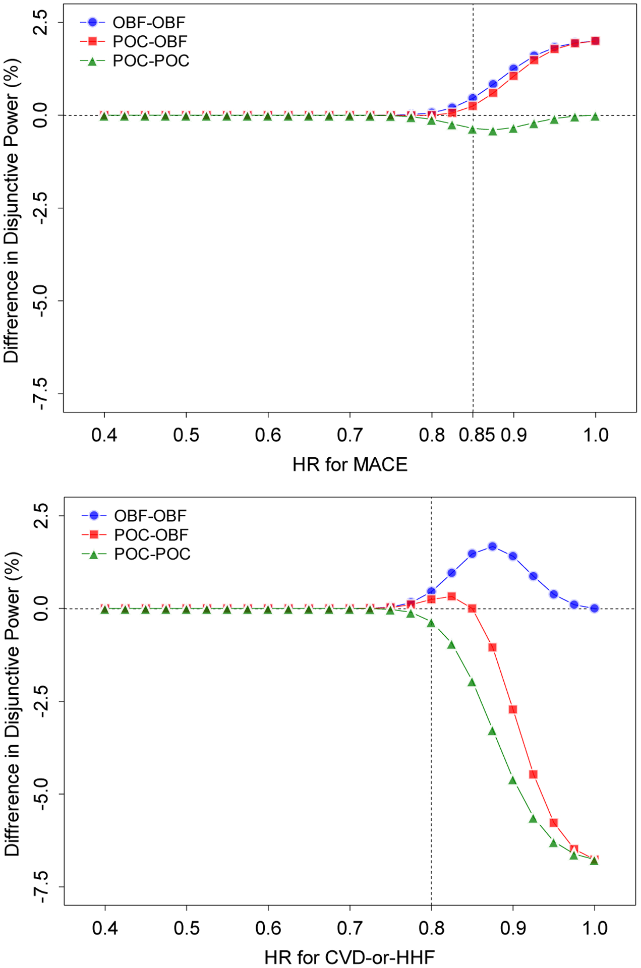
Hypothetical Example 1. Difference in disjunctive powers between critical boundary function combinations with varying HRs when the BH procedure is used, where OBF-POC is the reference and ρ =0.3. The upper panel (i) shows the conjunctive power as a function of the HR for MACE ψ₁ with the fixed HR for CVD-or-HHF ψ₂ =0.80, and the lower panel (ii) as a function of the HR for CVD-or-HHF ψ₂ with the fixed HR for MACE ψ₁ =0.85. The accrual duration is τ_A =36 months and follow-up duration is common for MACE and CVD-or-HHF, ${\tau }_{f_1}={\tau }_{f_2}={\tau }_f=24$ months. The HR is ψ₁ =0.85 for MACE and ψ₂ =0.80 for CVD-or-HHF. The proportion of survivors after the follow-up duration is common for MACE and CVD-or HHF $S_1^{(1)}(60)=S_2^{(1)}(60)=85\text{\%}$. Three analyses at 36, 48 and 60 months are planned for MACE and CVD-or HHF. The correlation is assumed to be ρ =0.3. The disjunctive power is calculated under a sample size of 14,466 with $S_1^{(1)}(60)=85\text{\%}$, which provides at least 80% power to detect 15% reduction in the HR for MACE at the 1.25% significance level by a one-sided logrank test in the fixed-sample design.

Figure 2.

Hypothetical Example 1. Difference in conjunctive powers between critical boundary function combinations with varying HRs when the BH procedure is used, where OBF-POC is the reference and ρ =0.3. The upper panel (i) shows the conjunctive power as a function of the HR for MACE ψ₁ with the fixed HR for CVD-or-HHF ψ₂ =0.80, and the lower panel (ii) as a function of the HR for CVD-or-HHF ψ₂ with the fixed HR for MACE ψ₁ =0.85. The accrual duration is τ_A =36 months and follow-up duration is common for MACE and CVD-or-HHF, ${\tau }_{f_1}={\tau }_{f_2}={\tau }_f=24$ months. The HR is ψ₁ =0.85 for MACE and ψ₂ =0.80 for CVD-or-HHF. The proportion of survivors after the follow-up duration is common for MACE and CVD-or HHF $S_1^{(1)}(60)=S_2^{(1)}(60)=85\text{\%}$. Three analyses at 36, 48 and 60 months are planned for MACE and CVD-or HHF. The correlation is assumed to be ρ =0.3. The conjunctive power is calculated under a sample size of 14,466 with $S_1^{(1)}(60)=85\text{\%}$, which provides at least 80% power to detect 15% reduction in the HR for MACE at the 1.25% significance level by a one-sided logrank test in the fixed-sample design.

For the disjunctive power, from Figure 1 (i), for most values of ψ₁, the highest power is attained by OBF-OBF and the lowest by POC-POC. However, there is no difference in powers between OBF-OBF and POC-OBF, and the maximum difference is 0.23%. All four powers behave similarly as ψ₁ approaches 0.4. The largest difference in power between OBF-OBF and OBF-POC is 2.0% when ψ₁ = 1.0. From (ii), similarly as in (i), for most values of ψ₂, the highest power is attained by OBF-OBF and the lowest by POC-POC. All four powers behave similarly as ψ₁ approaches 0.4. The largest difference in power between OBF-OBF and OBF-POC is 1.28% when ψ₂ = 0.875.

For the conjunctive power, from Figure 2 (i), in most of the range of ψ₁, the highest power is attained by OBF-OBF and the lowest by POC-POC. The power by OBF-POC behaves similarly to that by POC-POC, and the power by POC-OBF similarly to that by OBF-OBF as ψ₁ approaches 0.4. The largest difference in power between OBF-OBF and OBF-POC was 2.02% when ψ₁ <0.75. From (ii), similarly as in observed in (i), in most of the range of ψ₂, the highest power is attained by OBF-OBF and the lowest by POC-POC. The power by OBF-POC behaves similarly to the power by OBF-OBF, and the power by POC-OBF similarly to that by POC-POC as ψ₂ approaches 0.4. The largest difference in power between OBF-OBF and OBF-POC was 6.28% when ψ₂ =0.875.

The findings are summarized as follows:

• The selection of the boundary function affects disjunctive power. Regardless of the size of the reduction in HR for MACE or CVD-or-HHF, using OBF for both MACE and CVD-or-HHF, maximizes disjunctive power. When the effect sizes of endpoints are vastly different, using the POC for the endpoint with larger effect substantially decreases disjunctive power as the power is nearly determined by the endpoint with larger effect.

• The selection of the boundary function affects the conjunctive power. Regardless of the size of the reduction in HR for MACE or CVD-or-HHF, using OBF for both MACE and CVD-or-HHF maximizes conjunctive power. Using POC for the endpoint with larger effect and OBF for the other endpoint improves the conjunctive power, but its improvement is not larger than that by OBF for both endpoints. Using OBF for the endpoint with larger effect and POC for the other endpoint substantially decreases the conjunctive power.

• The correlation between the two endpoints does not appreciably affect both disjunctive and conjunctive powers.

3.2. Hypothetical Example 2

Consider a cancer clinical trial comparing two interventions with PFS (k =1) for short-term evaluation and OS (k =2) for long-term evaluation, where OS requires a longer follow-up duration than PFS. For illustration, we assume the following configurations and settings.

• FS procedure is used to test the null hypothesis of PFS and OS; the null hypothesis of PFS is first tested and then the null hypothesis of OS is tested only if the null hypothesis of PFS is rejected.

• The accrual duration is τ_A = 24 months and the follow-up durations vary between the two endpoints: ${\tau }_{f_1}=12$ month for PES and ${\tau }_{f_2}=36$ months for OS. The total duration of the trial is 60 months.

• The multiple interim analyses are preplanned, but the number and timings of analyses were different for the two endpoints: the two analyses at 24 and 36 months for PFS and up to the four analyses at 24, 36, 48 or 60 months for OS

• HR is ψ₁ = 0.65 for PFS and ψ₂ =0.70 for OS, with the proportion of survivors after the follow-up duration $S_1^{(1)}(36)=6.0\text{\%}$ and $S_2^{(1)}(60)=7.5\text{\%}$.

Table 4 summarizes the statistical information fraction and critical values for each endpoint with α = 2.5%, according to the above configurations and settings.

Table 4.

Hypothetical Example 2. Statistical information fraction and critical values

Endpoint	Statistical information fraction at τl;, critical boundary function	Calendar time τl; (in months) at lth analysis
		24 (l =1)	36 (l =2)	48 (l =3)	60 (l =4)
PFS	${\mathcal{J}}_1\left({\tau }_l\right)/{\mathcal{J}}_1\left({\tau }_2\right)$	0.6511	1.0
	OBF	2.5444	1.9898
	POC	2.0798	2.2427
OS	${\mathcal{J}}_2\left({\tau }_l\right)/{\mathcal{J}}_1\left({\tau }_4\right)$	0.4157	0.7053	0.8866	1.0
	OBF	3.2860	2.4353	2.1703	2.0647
	POC	2.2122	2.3083	2.3708	2.4142

The significance level is α = 2.5%. The accrual duration is τ_A =24 months and the follow-up duration is ${\tau }_{f_1}=12$ months for PFS and ${\tau }_{f_2}=36$ months for OS. The HRs ψ₁ =0.65 for PFS and ψ₂ =0.70 for OS. The proportion of survivors after the follow-up duration is $S_1^{(1)}(36)=6.0\text{\%}$ for PFS and $S_2^{(1)}(60)=7.0\text{\%}$ for OS. Two analyses at 24 and 36 months for PFS and up to four analyses at 24, 36, 48 or 60 months for OS are planned.

For this example, we discuss only the conjunctive power as the disjunctive power is determined by PFS when using FS procedure, and the selection of boundary function reduces to a single endpoint problem. Table 5 displays the stopping conjunctive probability at each analysis and overall conjunctive power for the four combinations of critical boundary functions for PFS and OS: (a) OBF for both PFS and OS (OBF-OBF); (b) OBF for PFS and POC for OS (OBF-POC); (c) POC for PFS and OBF for OS (POC- OBF); and (d) POC for both PFS and POC (POC-POC), when the FS procedure is used. A common correlation is assumed to be ρ =0.3, 0.5 and 0.8. The stopping probability and conjunctive power are calculated under a sample size of 304, which provides at least 80% power to detect 30% reduction in HR for OS at 2.5% significance level by a one-sided logrank test in the fixed-sample design (the total required number of OS events is 247).

Table 5.

Hypothetical Example 2. Stopping probability at each analysis and conjunctive power when the FS procedure is used.

Correlation	Boundary function combination	Stopping probability (%) at each analysis (month)				Conjunctive power (%)
		24 (l =1)	36 (l =2)	48 (l =3)	60 (l =4)
0.3	(a) OBF-OBF	4.52	36.62	19.92	10.53	71.59
	(b) OBF-POC	20.31	19.89	9.95	15.13	65.29
	(c) POC-OBF	5.60	35.69	19.23	8.97	69.49
	(d) POC-POC	25.90	19.21	9.44	9.25	63.79
0.5	(a) OBF-OBF	5.06	37.39	20.18	10.10	72.73
	(b) OBF-POC	21.88	20.14	10.10	14.27	66.39
	(c) POC-OBF	6.01	36.65	19.49	8.68	70.82
	(d) POC-POC	27.20	19.54	9.58	8.83	65.15
0.8	(a) OBF-OBF	6.12	38.92	20.98	9.22	75.25
	(b) OBF-POC	25.39	21.05	10.56	11.65	68.65
	(c) POC-OBF	6.68	38.65	20.41	8.12	73.87
	(d) POC-POC	29.95	20.61	10.07	7.47	68.11

The accrual duration is τ_A =24 months and the follow-up duration is ${\tau }_{f_1}=12$ months for PFS and ${\tau }_{f_2}=36$ months for OS. The HR is ψ₁ =0.65 for PFS and ψ₂ =0.70 for OS. The proportion of survivors after the follow-up duration is $S_1^{(1)}(36)=6.0\text{\%}$ for PFS and $S_2^{(1)}(60)=7.0\text{\%}$ for OS. Two analyses at 24 and 36 months for PFS and up to four analyses at 24, 36, 48 or 60 months for OS are planned. A correlation is assumed to be ρ =0.3, 0.5 and 0.8. The conjunctive probability at each anal and conjunctive power are calculated under a sample size of 304, which provides at least 80% power to detect 30% reduction in the HR for OS at the 2.5% significance level by a one-sided logrank test in the fixed-sample design.

All four powers slightly increase with higher correlation and the order of the powers for the four combinations is the same. The highest power is attained by OBF-OBF and the lowest by POC-POC. Unlike Example 1, the power by OBF-POC is approximately 6.3% smaller than that by OBF-OBF. The stopping probability distribution is different for OBF-OBF and OBF-POC. The highest stopping probability by OBF-OBF is at the second analysis and the first analysis by OBF-POC.

Further investigation was conducted to evaluate the behavior of conjunctive power with varying HRs i for the combinations of critical boundary function. Figure 3 displays difference in the conjunctive power between critical boundary function combinations, with varying HRs (from 0.4 to 1.0), where OBF-POC is the reference and ρ =0.3. The upper panel (i) shows the conjunctive power as a function of HR for PFS ψ₁ with the fixed HR for OS ψ₂ =0.70, and the lower panel (ii) as a function of HR for OS ψ₂ with the fixed HR for PFS ψ₁ =0.65.

Figure 3.

Hypothetical Example 2. Difference in conjunctive powers between critical boundary function combinations with varying HRs when the FS procedure is used, where OBF-POC is the reference and ρ =0.3. The upper panel (i) shows the conjunctive power as a function of HR for PFS ψ₁ with the fixed HR for OS ψ₂ =0.70, and the lower panel (ii) as a function of HR for OS ψ₂ with the fixed HR for PFS ψ₁ =0.65. The accrual duration is τ_A =24 months and the follow-up duration is ${\tau }_{f_1}=12$ months for PFS and ${\tau }_{f_2}=36$ months for OS. The HR is ψ₁ =0.65 for PFS and ψ₂ =0.70 for OS. The proportion of survivors after the follow-up duration is $S_1^{(1)}(36)=6.0\text{\%}$ for PFS and $S_2^{(1)}(60)=7.0\text{\%}$ for OS. Two analyses at 24 and 36 months for PFS and up to four analyses at 24, 36, 48 or 60 months for OS are planned. A correlation is assumed to be ρ =0.3. The conjunctive power is calculated under a sample size of 304, which provides at least 80% power to detect 30% reduction in the HR for OS at the 2.5% significance level by a one-sided logrank test in the fixed-sample design.

From (i), in most of the range of ψ₁, the highest power is attained by OBF-OBF and the lowest by POC-POC, and the power by OBF-POC is smaller than that by OBF-OBF or POC-OBF. The largest difference in power between OBF-OBF and OBF-POC is 6.68% when ψ₁ =0.575. The power by OBF-POC behaves similarly to that by POC-POC, and the power by POC-OBF behaves similarly to that by OBF-OBF as ψ₁ approaches 0.4. From (ii), similarly as in (i), in most of the range of ψ₂, the highest power is attained by OBF-OBF and the lowest by POC-POC. The power by OBF-POC is smaller than that by OBF-OBF in most of the range of ψ₂. In addition, when ψ₂ >0.625, the power by OBF-POC is smaller than that by POC-OBF. The largest difference in power between OBF-OBF and OBF-POC is 7.46% when ψ₂ =0.75. The power by OBF-POC behaves similarly to that by POC-POC, and the power by POC-OBF similarly to that by OBF-OBF as ψ₂ approaches one.

Figure 4 displays the difference in conjunctive power between critical boundary function combinations with varying HRs and the proportion of survivors when the FS procedure is used, where OBF-POC is the reference and ρ =0.3. This is modified from Example 2 above: the follow-up durations, ${\tau }_{f_1}=8$ months for PFS and ${\tau }_{f_2}=40$ months for OS; and the timing of analyses, the two analyses at 17 and 32 months for PFS and up to the four analyses at 17, 32, 49 or 64 months for OS; and the proportion of survivors after the follow-up duration, $S_1^{(1)}(32)=6.25\text{\%}$ for PFS and $S_2^{(1)}(64)=7.36\text{\%}$ for OS. The upper panel (i) shows the conjunctive power as a function of HR for PFS ψ₁ with the fixed HR for OS ψ₂ =0.70, and the lower panel (ii) as a function of HR for OS ψ₂ with the fixed HR for PFS ψ₁ =0.62. The conjunctive power is calculated under a sample size of 348, which provides at least 80% power to detect 30% reduction in the HR for OS at the 2.5% significance level by a one-sided logrank test. From (i), for most values of ψ₁, the highest power is attained by POC-OBF and the lowest by OBF-POC. The largest difference in power between POC-OBF and OBF-POC is 6.55 % when ψ₁ = 0.75. The power by OBF-OBF behaves similarly to that by POC-OBF, and POC-POC behaves similarly to that by OBF-POC as ψ₁ approaches 0.4. From (ii), similarly as in (i), for most values of ψ₂, the highest power is attained by POC-OBF and the lowest by OBF-POC. The largest difference in power between POC-OBF and OBF-POC is 5.12% when ψ₂ = 0.75. The power by OBF-OBF behaves similarly to that of POC-OBF and the difference in power between OBF-OBF and POC-OBF becomes larger as ψ₁ approaches 0.4, although it is relatively small (i.e., the maximum difference is approximately 1.0%).

Figure 4.

Difference in conjunctive powers between critical boundary function combinations with varying HRs and proportion of survivors when the FS procedure is used, where OBF-POC is the reference and ρ =0.3. The upper panel (i) shows the conjunctive power as a function of HR for PFS ψ₁ with the fixed HR for OS ψ₂ =0.70, and the lower panel (ii) as a function of HR for OS ψ₂ with the fixed HR for PFS ψ₁ =0.60. The accrual duration is τ_A = 24 months and the follow-up duration is ${\mathit{\tau }}_{{\mathit{f}}_{\mathbf{1}}}=8$ months for PFS and ${\mathit{\tau }}_{{\mathit{f}}_{\mathbf{2}}}=40$ months for OS. The two analyses at 17 and 32 months for PFS and up to four analyses at 17, 32, 49 or 64 months for OS are planned. The proportion of survivors after the follow-up duration is ${\mathit{S}}_{\mathbf{1}}^{(\mathbf{1})}(\mathbf{32})=6.25\text{\%}$ for PFS and ${\mathit{S}}_{\mathbf{2}}^{(\mathbf{1})}(\mathbf{64})=7.36\text{\%}$ for OS. The conjunctive power is calculated under a sample size of 348, which provides at least 80% power to detect 30% reduction in the HR for OS at the 2.5% significance level by a one-sided logrank test.

The findings are summarized as follows:

• The selection of the boundary functions affects the conjunctive power. Using OBF for PFS and POC for OS substantially decreases the conjunctive power.

• Using OBF for both PFS and OS generally maximizes conjunctive power. Also using POC for PFS and OBF for OS improves the conjunctive power, but in most situations, its improvement may not be larger than that by OBF for both endpoints.

• The correlation between the two endpoints and the timings of analyses do not appreciably affect the conjunctive power.

4. Summary and points to consider

We discussed the selection of critical boundary functions for testing the hypotheses associated with two time-to-event outcomes as both primary endpoints, or a primary and a secondary endpoint, in group-sequential clinical trials, where (1) the effect sizes of the two endpoints are unequal, or (2) one endpoint represents short-term evaluation and the other long-term evaluation. We considered Bonferroni-Holm (non-hierarchical) or the fixed-sequence (hierarchical) procedure for testing these hypotheses. We evaluated the behavior of conjunctive power in selecting the critical boundary functions for two endpoints and assessed the effect of the sizes of the HRs and the correlation between the endpoints on the power.

For testing two time-to-event endpoints, using the OBF boundary function for the primary endpoint and the POC boundary function for the secondary endpoint does not appear to be able to maximize the conjunctive power, compared to other combinations of critical boundary functions when the fixed-sequence procedure is used. In addition, when Bonferroni-Holm procedure is used to test the hypotheses associated with two primary endpoints, using different critical boundary functions cannot improve the disjunctive and conjunctive powers.

The following points can be considered during the selection of critical boundary functions for testing two time-to-event endpoints in group-sequential trials.

• OBF is recommended for testing endpoints to maximize the disjunctive power when a non-hierarchical testing procedure is used to test the hypotheses associated with the two endpoints. POC is not recommended for the endpoint with larger effect as it substantially decreases disjunctive power.

• When a hierarchical or non-hierarchical testing procedure is used to test the hypotheses associated with the two endpoints, in general, OBF can be recommended for testing both endpoints to maximize the conjunctive power. This combination generally attains the highest powers among the combinations.

• When one endpoint is for short-term evaluation and other for long-term evaluation, or the two endpoints have drastically different effect sizes, using POC is not recommended for the long-term endpoint or the endpoint with a smaller effect size, regardless of whether a hierarchical or non-hierarchical testing procedure is used. With POC, α is spent substantially at early analyses resulting in a substantial decrease in the conjunctive power. For such endpoints, OBF provides higher conjunctive power.

• When considering the primary for short-term evaluation and secondary for long-term evaluation, if a hierarchical testing procedure is used, it is worth considering different critical boundary functions to improve the conjunctive power, e.g., POC for the short-term endpoint and OBF for the long-term endpoint. However, the conjunctive power is affected by the extent of the HR reduction, the number and timing of analyses, the length of accrual and follow-up and durations, duration, and the proportion of survivors. Careful evaluation is required.

As shown in Section 3, use of different critical boundary functions (OBF-POC or POC-OBF) tends to reject either or both of the null hypotheses at an earlier analysis, compared with OBF-OBF. This may contribute efficiency improvement (i.e., smaller average sample numbers or event numbers). In practice, the values of effect sizes and other related design parameters used for designing a trial are generally unknown. Prior data may help estimate these values. Such data may often be limited. Earlier decisions based on limited data may generate results with larger bias. As shown in Section 3, in most situations, OBF-POC or POC-OBF provides lower overall disjunctive and conjunctive powers than OBF-OBF. Due to these reasons, OBF-OBF would be generally recommended in practice. When using different critical boundary functions, careful consideration is required.

In this paper, using time-to-event clinical trial examples, we illustrated the power behaviors with combinations of critical boundary functions for testing the hypotheses. The points to consider given above provide useful advice for designing clinical trials for continuous or binary endpoints, particularly when a trial continues to test the null hypothesis of the other primary or secondary endpoint even if the null hypothesis of a primary endpoint is rejected at an interim analysis. Designing clinical trials for time-to-event endpoints is more complex than designing clinical trials for continuous or binary endpoints. Careful consideration is definitely needed for designing such trials. In addition to the effect sizes, other design factors that need to be considered include the length of accrual and follow-up durations, the proportion of non-censoring, censoring scheme, and the relationship between the two endpoints, all of which are very likely to affect the power and required sample size. An extensive evaluation of the power performances with such factors will aid decision-making when selecting critical boundary functions for testing time-to-event endpoints.

In the hypothetical examples discussed in Section 3, the outcomes (MACE and CVD-or-HHF, or PFS and OS) are composite of multiple outcomes including death event as its component, or death itself. In these examples, one endpoint is still observed even if the other endpoint is completely observed. For example, PFS can be still observed even when OS is observed as PFS includes OS as its component. On the other hand, in clinical trials with one fatal and non-fatal time-to-event outcomes as primary endpoints, or a primary or a secondary endpoint, semi-competing risk issues will arise, where the “fatal” event impedes occurrence of future events of interest. For example, in oncology trials utilizing TTP and OS as primary endpoints, TTP is censored by OS being completely observed before TTP. If there is a non-zero correlation between the endpoints (i.e., dependent censoring), the dependence in censoring requires to modify the log-rank statistics and thus the statistical information of non-fatal events (TTP) and the correlation structure of group-sequential log-rank statistics for the two endpoints. Further investigation will be required to assess the power behavior with selection of critical boundary functions for testing the hypotheses concerning semi-competing time-to-event outcomes.

For co-primary endpoints, where a trial is designed to evaluate a joint effect on all of the primary endpoints, similarly to the situation discussed in this paper, a trial continues until the null hypotheses of all endpoints have been rejected. However the multiple testing procedures such as the BH and FS procedures will not be required for controlling the Type I error in testing the null hypotheses of the co-primary endpoints. The hypotheses for all endpoints should be tested at the same significance level of α. Further investigation will be required, particularly when there are differences in statistical information at a particular interim time-point of the trial, follow-up duration, or number and timing of analyses for the endpoints. Some discussion on the combination of critical boundary functions for testing the hypothesis can be found in Asakura et al. [17, 18] and Hamasaki et al. [19].

References

- [1].Glimm EE, Maurer W, Bretz F. Hierarchical testing of multiple endpoints in group-sequential trials. Statistics in Medicine, 29 (2010), pp. 219–228. doi: 10.1002/sim.3748. [DOI] [PubMed] [Google Scholar]
- [2].Tamhane AC, Mehta CR, Liu L. Testing a primary and secondary endpoint in a group sequential design. Biometrics, 66 (2010), pp. 1174–1184. doi: 10.1111/j.1541-0420.2010.01402.x. [DOI] [PMC free article] [PubMed] [Google Scholar]
- [3].O’Brien PC, Fleming TR. A multiple testing procedure for clinical trials. Biometrics, 5 (1979), pp. 549–556. doi: 10.2307/2530245 [DOI] [PubMed] [Google Scholar]
- [4].Pocock SJ. Group sequential methods in the design and analysis of clinical trials. Biometrika, 64 (1977), pp. 191–199. doi: 10.2307/2335684 [DOI] [Google Scholar]
- [5].Hung HMJ, Wang SJ, Yang P, Jin K, Lawrence J, Kordzakhia G, Massie T. Statistical challenges in regulatory review of cardiovascular and CNS clinical trials. Journal of Biopharmaceutical Statistics, 26 (2016), pp. 37–43. doi: 10.1080/10543406.2015.1092025 [DOI] [PubMed] [Google Scholar]
- [6].Gou J, Xi D. Hierarchical testing of a primary and a secondary endpoint in a group sequential design with different information times. Statistics in Biopharmaceutical Research, 11 (2019), pp. 398–406. doi: 10.1080/19466315.2018.1546613 [DOI] [Google Scholar]
- [7].Sugimoto T, Hamasaki T, Halabi S, Evans SR. Group-sequential logrank methods for trial designs using bivariate non-competing event-time outcomes. Lifetime Data Analysis, 26 (2020), pp. 266–291. doi: 10.1007/s10985-019-09470-4 [DOI] [PMC free article] [PubMed] [Google Scholar]
- [8].Hung HMJ, Wang SJ, O’Neill R. Statistical considerations for testing multiple endpoints in group sequential or adaptive clinical trials. Journal of Biopharmaceutical Statistics, 17 (2007), pp. 1201–1210. doi: 10.1080/10543400701645405 [DOI] [PubMed] [Google Scholar]
- [9].Maurer W, Bretz F. Multiple testing in group sequential trials using graphical approaches. Statistics in Biopharmaceutical Research, 5 (2013), pp. 311–320. doi: 10.1080/19466315.2013.807748 [DOI] [Google Scholar]
- [10].Xi D, Tamhane AC. Allocating recycled significance levels in group sequential procedures for multiple endpoints. Biometrical Journal, 57 (2015), pp. 90–107. doi: 10.1002/bimj.201300157 [DOI] [PubMed] [Google Scholar]
- [11].Ye Y, Li A, Liu L, Yao B. A group sequential holm procedure with multiple primary endpoints. Statistics in Medicine, 32 (2013), pp.1112–1124. doi: 10.1002/sim.5700 [DOI] [PubMed] [Google Scholar]
- [12].Hamasaki T, Asakura K, Evans SR, Ochiai T. Interim evaluation of efficacy in clinical trials with two primary endpoints. In Group-Sequential Clinical Trials with Multiple Co-Objectives, pp. 67–80, 2016, Springer. doi: 10.1007/978-4-431-55900-9_5 [DOI] [Google Scholar]
- [13].Lan KKG, DeMets DL. Discrete sequential boundaries for clinical trials. Biometrika, 70 (1983), pp. 659–663. doi: 10.1093/biomet/70.3.659. doi: 10.1016/S1470–2045(13)70158-X [DOI] [Google Scholar]
- [14].Reboussin DM, DeMets DL, Kim KM, Lan KKG. Computations for Group Sequential Boundaries Using the Lan-DeMets Spending Function Method. Contemporary Clinical Trials, (200) 21, pp.190–207. doi: 10.1016/S0197-2456(00)00057-X. .. [DOI] [PubMed] [Google Scholar]
- [15].Clayton DG. A model for association in bivariate life tables and its application in epidemiological studies of familial tendencyin chronic disease. Biometrika, 65 (1976), 6, pp.141–151. doi: 10.1093/biomet/65.1.141 [DOI] [Google Scholar]
- [16].Mauguen A, Pignon JP, Burdett S, Domerg C, Fisher D, Paulus R, Mandrekar SJ, Belani CP, Shepherd FA, Eisen T, Pang H, Collette L, Sause WT, Dahlberg SE, Crawford J, O’Brien M, Schild SE, Parmar M, Tierney JF, Le Pechoux C, Michiels S, on behalf of the Surrogate Lung Project Collaborative Group. Surrogate endpoints for overall survival in chemotherapy and radiotherapy trials in operable and locally advanced lung cancer: a re-analysis of meta-analyses of individual patients’ data. Lancet Oncology, 14 (2013) pp. 619–626. doi: 10.1016/S1470-2045(13)70158-X. [DOI] [PMC free article] [PubMed] [Google Scholar]
- [17].Asakura K, Hamasaki T, Sugimoto T, Hayashi K, Evans SR, Sozu T. Sample size determination in group-sequential clinical trials with two co-primary endpoints. Statistics in Medicine, 33 (2014), pp. 2897–2913. doi: 10.1002/sim.6154. [DOI] [PMC free article] [PubMed] [Google Scholar]
- [18].Asakura K, Hamasaki T, Evans SR, Interim T evaluation of efficacy or futility in group-sequential trials with multiple co-primary endpoints. Biometrical Journal 59 (2017), pp.703–731. doi: 0.1002/bimj.201600026 [DOI] [PMC free article] [PubMed] [Google Scholar]
- [19].Hamasaki T, Asakura K, Evans SR, Sugimoto T, Sozu T. Group-sequential strategies in clinical trials with multiple co-primary outcomes. Statistics in Biopharmaceutical Research, 7 (2015), pp. 36–54. doi: 10.1080/19466315.2014.1003090 [DOI] [PMC free article] [PubMed] [Google Scholar]