HeadLocNet: Deep Convolutional Neural Networks for Accurate Classification and Multi-landmark Localization of Head CTs

Abstract

Cochlear implants (CIs) are used to treat subjects with hearing loss. In a CI surgery, an electrode array is inserted into the cochlea to stimulate auditory nerves. After surgery, CIs need to be programmed. Studies have shown that the cochlea-electrode spatial relationship derived from medical images can guide CI programming and lead to significant improvement in hearing outcomes. We have developed a series of algorithms to segment the inner ear anatomy and localize the electrodes. But, because clinical head CT images are acquired with different protocols, the field of view and orientation of the image volumes vary greatly. As a consequence, visual inspection and manual image registration to an atlas image are needed to document their content and to initialize intensity-based registration algorithms used in our processing pipeline. For large-scale evaluation and deployment of our methods these steps need to be automated. In this article we propose to achieve this with a deep convolutional neural network (CNN) that can be trained end-to-end to classify a head CT image in terms of its content and to localize landmarks. The detected landmarks can then be used to estimate a point-based registration with the atlas image in which the same landmark set’s positions are known. We achieve 99.5% classification accuracy and an average localization error of 3.45mm for 7 landmarks located around each inner ear. This is better than what was achieved with earlier methods we have proposed for the same tasks.

Graphical Abstract

1. Introduction

1.1. Clinical background and motivation of this work

Cochlear implants (CIs) have been among the most successful neural prosthetics developed in the past few decades (NIDCD 2011). They are used to treat subjects with severe-to-profound hearing loss. During a cochlear implantation surgery, an array of electrodes is threaded into the cochlea to replace the natural sound transduction mechanism of the human hearing system. After surgery, the CI needs to be programmed for hearing outcome optimization. This process includes the assignment of a frequency range to each individual contact in the array so that it is activated when the incoming sound includes frequency components in such a range. Traditionally, the programming is done by an audiologist who can only rely on the recipients’ subjective response to certain stimuli, e.g., whether they can hear a signal or rank pitches, without other clues. Accurate localization of electrodes in the CI relative to the intra-cochlear anatomy can provide useful guidance to audiologists to adjust the CI programming. Recently, our group has developed an image-guided cochlear implant programming (IGCIP) system (Noble et al. 2013). It includes algorithms that permit the accurate segmentation of the intra-cochlear anatomy (Noble et al. 2011) and the localization of CI electrodes in clinical head CTs (Zhao et al. 2018)(Zhao et al. 2019). Studies in (Noble et al. 2014)(Noble et al. 2016) have shown that the use of image guidance to program the CI leads to a significant improvement in hearing outcomes for both adults and children.

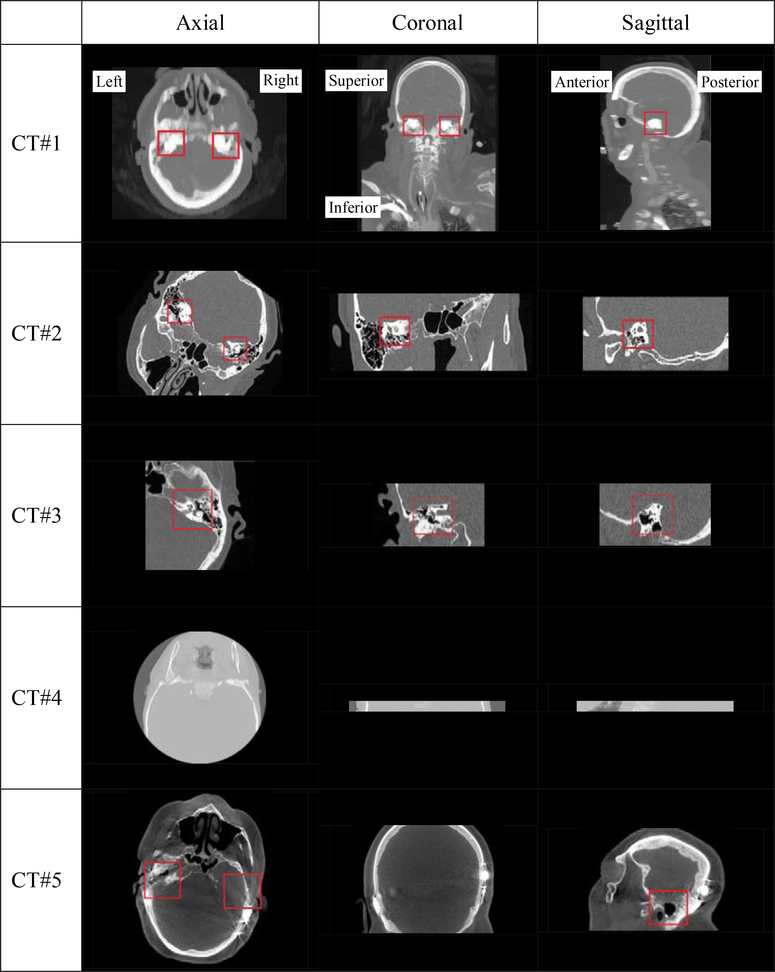
At the time of writing our IGCIP system is not yet fully automated, which hampers its large scale clinical deployment. One hurdle is the heterogeneity of the clinical head CTs that can be acquired on a variety of scanners with a range of acquisition protocols from multiple sites. Because of this the field of view (FOV) and orientation of the CT volumes vary greatly. Fig. 1 shows several representative examples. Here, CT#1 covers a very large FOV, including both the whole head and the upper part of the torso. The FOV of CT#2 is representative of most (~80%) CTs in our image repository, but the head orientation deviates a lot from the most common pose shown in CT#1. CT#3 has a smaller FOV which only includes the right inner ear. In CT#4, only a narrow horizontal portion of the head is imaged and neither inner ear is included. The lack of a standard acquisition protocol also affects image contrast and quality as shown in Fig. 1 where CT#1 is visibly of lower quality than the three others. CT #5 is a post-operative CT and serious beam hardening artifacts caused by the electrode arrays are visible. This poses an additional challenge.

Fig. 1.

Five representative CT volumes included in our dataset. The inner ears are shown in red boxes if they are present in the volume and visible in the slice

Because of the heterogeneity we describe above, manual intervention is often needed in our system prior to applying automatic algorithms to the images. First, when a new CT volume is received, a human operator needs to document manually its content, i.e., which ear(s) is/are included in the volume; this is needed by model-based algorithms we use to segment the inner ear structures. Second, because our processing pipeline includes several rigid and non-rigid Mutual Information (MI)-based registration algorithms that require a reasonable initial alignment, manual intervention, i.e., manual translation and rotation of the images can be required. Our ultimate goal is to develop a series of algorithms that are robust and fully automatic. In this work, we focus on developing methods to document the image content and to localize a set of landmarks that can be used for the estimation of an initial transformation that registers an atlas with a new volume using point-based registration techniques.

1.2. Related Works

Detecting landmarks in medical images has been a well-studied topic for many years. The reader is referred to the work of Rohr for a review of earlier work (Rohr 2001). In the past few years, learning-based methods have been successfully applied to this task starting with random forest–based methods (Breiman 2001). An exhaustive review of this body of work would be outside the scope of this article but some representative papers include (Donner et al. 2013)(Zheng et al. 2012)(Criminisi et al. 2013)(Han et al. 2015)(Ebner et al. 2014)(Lindner et al. 2016)(Zhang et al. 2016).

Recently, convolutional neural networks (CNNs) have superseded random forest techniques for a range of applications. Originally developed for 2D images, they have been expanded to 3D and the 3D U-Net architecture proposed by (Çiçek et al. 2016) has been widely used for medical image segmentation and detection tasks. Again, a complete coverage of this body of work would be outside the scope of this article but examples that are germane to our work include the work of Payer et al. (Payer et al. 2016) who have proposed a “SpatialConfiguration-Net” to detect landmarks in MR volumes, of Zhang et al. (Zhang et al. 2017b) who have devised a system that consists of two 3D deep networks for both brain and prostate landmark detection, of Yang et al, (Yang et al. 2017) who used a volume-to-volume network to detect a set of vertebra points in 3D CT volumes, and of Liu et al. (Liu et al. 2018) who used a 3D network to detect landmarks in the brain for disease diagnosis.

Multi-tasking CNNs have also been proposed for medical image processing and analysis tasks. Such convolutional network models typically start with several shared hidden layers from the input side and branch to multiple paths, each leading to one output. They can be trained using a combination of loss functions, each computed from one output. Deep multi-task learning can reduce the risk of overfitting caused by learning from single tasks because of the regularization effect that each task has on others. For instance, (Xu et al. 2018) proposed to do localization and view classification of abdominal ultrasound images in a single 2D network. (Mehta et al. 2018) proposed to learn segmentation and classification of 2D breast biopsy images simultaneously. Finally, Deep Reinforcement Learning (DRL) has been used recently to design methods for landmark detection in 3D medical images. (Maicas et al. 2017) have proposed to use DRL to detect breast lesion in DCE-MRI images. Ghesu et al. have proposed to use DRL to detect anatomical landmarks in incomplete volumetric images in (Ghesu et al. 2018) and later in (Ghesu et al. 2019). This approach, which has been tested on landmarks ranging from kidney center to bronchial bifurcation compares favorably to several deep learning methods proposed earlier by these authors and others.

Our own work has been focused on developing robust automated methods for head CT images and more specifically on the documentation of images covering the ears and on the localization of landmarks in these images to initialize registration algorithms. We have proposed methods to perform image content documentation and registration initialization tasks separately. These are presented in (Zhang et al 2018a), and (Zhang et al. 2017a), respectively. In the former article, the content of head CT volumes is documented using a 2D CNN. The CT volume is processed slice by slice or in very thin 3D volumes (3 consecutive slices). This makes the algorithm computationally inefficient and full 3D information is not exploited. As will be shown in the results section, the solution we propose herein leads to better results. In the latter paper, we estimate a rigid-body transformation via a set of landmarks but the system was not designed to document image content. The evaluation is also done on a screened dataset in which each image includes the region of interest, i.e., a region that encompasses the ear.

In the work reported herein, which is an extension of our MICCAI conference paper (Zhang et al. 2018b), we use a deep multi-task learning algorithm in an end-to-end fashion. The algorithm we propose can map a CT volume to a four-way classifier which accurately predicts whether the volume includes both inner ears, only the right inner ear, only the left inner ear, or neither, and simultaneously generates probability maps that indicate the positions of a set of landmarks around each inner ear.

The novel aspects we present in this article are: (1) the number of landmarks surrounding each inner ear is augmented from one to seven. By doing this, instead of only being able to find the positions of the inner ears, we can estimate a local rigid-body transformation between the image volume and an atlas to initialize our MI-based registration. (2) Instead of only using the maximum response of the final network output to document the volume content as we did earlier, we add a classification branch that is specially designed to perform this task. We use feature maps at different levels as input to the classification branch and train the classification branch. We show that such hierarchical features improve the image classification accuracy. (3) Thanks to the new architecture and a modification of the loss function we use to train our network, we do not need the post-processing steps that were required previously to eliminate false positives.

In the following sections, we succinctly describe our earlier work in the conference paper, present improvements we have brought to this early solution, and compare the two approaches.

2. Materials

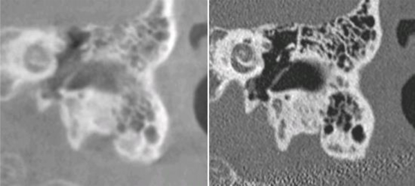
The data we use in this study include head CTs from 322 subjects. Since images were acquired both pre-operatively and post-operatively, and multiple reconstructions can be performed for one acquisition, more than one CT volume can pertain to a subject. Also, different CT volumes pertaining to a subject can have different fields of view. In total, we have used 1,593 CT volumes in this study. The scanners that were used to acquire these images include both conventional and Xoran xCAT® scanners. Xoran xCAT® scanners are flat-panel, low-dose Cone Beam CT (CBCT) scanners. Compared to CTs acquired with conventional scanners, images acquired with such scanners typically have lower quality and suffer from intensity inhomogeneity. We refer to CT image volumes they produce as lCTs and CT image volumes acquired with conventional CTs as convCTs. One typical lCT and one typical convCT obtained from the same subject and rigidly registered to each other are shown in Fig. 2 to illustrate differences between them. The volumes in our data set also cover regions of different sizes and have different resolutions. The size ranges from 10 mm to 256 mm in the left-right and anterior-posterior directions and from 52 mm to 195 mm in the inferior-superior direction. The resolution varies from 0.14 mm to 2.00 mm in the left-right and anterior-posterior directions and from 0.14 mm to 5.00 mm in the inferior-superior direction.

Fig. 2.

A comparison of lCT (left) and convCT (right) from the same subject, in the ear region.

To develop and evaluate our proposed method, we randomly split the data into a training set and a testing set. We verify that image volumes pertaining to a single subject are not split between the two sets. The numbers of CT volumes in the training set and the testing set are listed in the upper part of Table 1. The images are categorized according to whether they are convCTs or lCTs and whether they contain an implant (w/ CI) or not (w/o CI).

Table 1.

Distributions ot our CT data w.r.t. the presence of CI and scanner type before and after augmentation

	Training data					Test data
	convCT w/ CI	lCT w/ CI	convCT w/o CI	lCT w/o CI	Total	convCT w/ CI	lCT w/ CI	convCT w/o CI	lCT w/o CI	Total
Before	125	146	527	0	798	102	140	553	0	795
After	155	253	1871	323	2602	150	239	1786	321	2496

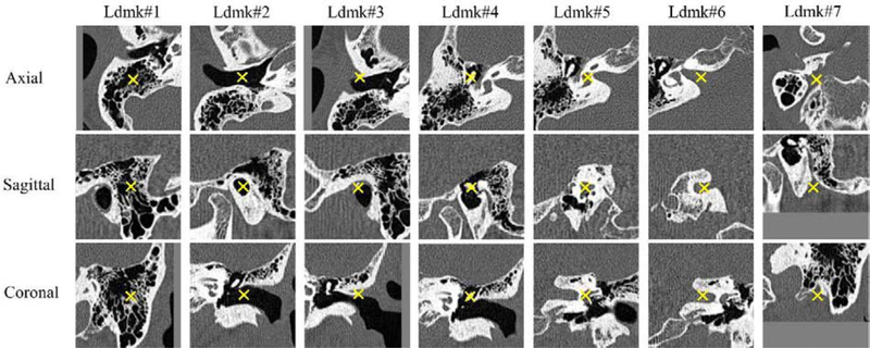
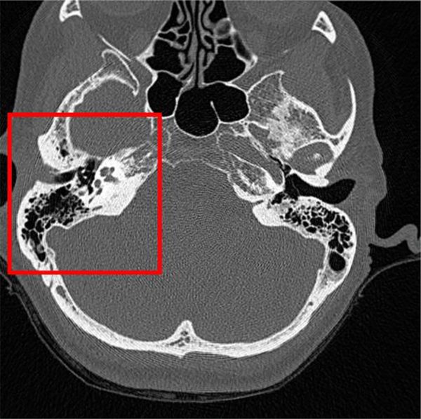
For each volume, we visually check the presence of inner ears. For each visible inner ear, 7 pre-defined landmark points surrounding the cochlea are manually selected. They represent the positions of the mastoid, the external auditory canal, the spine of henle, the ossicles, the cochlear labyrinth, the internal auditory canal, and the stylomastoid foramen. They are shown in Fig. 4. The region of interest is shown in Fig. 3. As mentioned earlier, scans can include both inner ears, only one (left/right), or neither. However, the number of image volumes in each of these four categories is not balanced. Indeed, in our current data set about 80% of the volumes include both ears. About 20% include one inner ear. Image volumes that include neither inner ear exist but are rare. To tackle this issue, we augment each set by cropping sub-volumes from CT volumes that include both ears to create artificial samples for the other three categories. An affine transformation (i.e., scaling, rotation and skewing) is applied to the cropped images. The scaling, rotation and skewing parameters along and around each axis are randomly generated by uniformly sampling values in intervals [0.95, 1.05], [−5°, 5°] and [0, 0.05], respectively. Typically, these operations are used for data augmentation in the training phase. Here we do the same for the testing set to increase its variability and to test the network on a sizeable number of cases in each category. All image volumes are resampled to 2.25×2.25×2.25 mm³/voxel. It is a convention in deep learning to map the image intensity to [−1, 1] (or [0, 1]) by applying a linear scaling operation that converts the maximum intensity to 1 and the minimum to −1. In our dataset, the intensity of metal implants in post-operative CTs is much higher than that of normal human tissue. Applying a linear scaling would compress the intensity range of the tissues and potentially affect the training of the network. To avoid this issue, we first apply an intensity cutoff, i.e., we set the intensity values of the 0.1% voxels with the highest intensities (an empirical estimation of the fraction of voxels occupied by the metal implant) to their lower bound. We subsequently apply the intensity remapping. All images are cropped or padded to 96×96×96 voxels. This size fits the input of the 3D U-Net and is big enough to include the whole head with the voxel size we use. The number of volumes in each category in the training and testing sets after augmentation is shown in the lower part of Table 1. It shows that our data set does not contain pre-operative lCT volumes. This is because the flat-panel scanner is only used to acquire post-operative images. As a consequence, our lCT pre-operative images in the augmented training and testing sets only include volumes that contain a single ear. These have been generated from unilateral post-operative volumes. In the testing set, there are 625, 625, 625 and 621 CTs that include both, left, right and neither ear(s), respectively. The number of subjects in each of the four categories in the testing set is 153, which is also the total number of patients in the set. As mentioned above, multiple CT images with different FOVs are often associated with a single subject. Each subject in our testing set has at least a “both-ear” CT. We crop “single-ear” volumes or a “neither-ear” volume if there is no such image in the original set.

Fig. 4.

The seven landmarks that have been selected for the study. “Ldmk” is used for “Landmark”

Fig. 3.

The region in which the landmarks are selected

3. Methods

3.1. HeadLocNet-1: Inner Ear Detection Using the 3D U-Net with False Positive Suppression and a Shape Constraint

In this first solution presented in (Zhang et al. 2018b) and repeated partially here for the sake of clarity and completeness, we formulate the inner ear detection problem as a single landmark detection problem. We use the fifth landmark, i.e., the one representing the cochlear labyrinth, in the set of seven shown in Fig. 4 because it is the closest to the cochlea and we use the 3D U-Net proposed by (Çiçek et al. 2016) to map a whole 3D image volume to two probability maps, one for each ear, that have the same dimensions as the input volumes. The 3D U-Net requires a 3D volume as input. The network consists of a sequence of convolution-pooling layers which compress the raw input volume into low-resolution, highly-abstracted feature maps. Following them are a sequence of convolution-upsampling layers, which process the abstracted feature maps into outputs with the same resolution as the input, in a way that is symmetrical to what is done in the compression layers. In our first attempt, at the training stage, for each inner ear, we use a 3D Gaussian function centered at the manually labeled landmark position as a probability map. The standard deviation σ of the Gaussian is empirically set to 3 voxels in the resampled image. The probability values are multiplied by a constant to scale the maximum to 1. Any value below 0.05 is set to 0. If the inner ear is not included in the image, all values in the corresponding probability map are set to 0. We treat this volume-to-volume mapping as a voxel-wise regression problem. The weighted mean of voxel-wise squared errors between the output probability maps and those generated with the ground truth inner ear landmarks is used as the loss function. Larger weights are assigned to voxels with non-zero probabilities in the supervising maps. They are sparse but are very important features. Specifically, suppose the numbers of non-zero entries and zero entries are N_nonzero and N_zero, respectively, in the output probability map. The weights associated with non-zero entries and zero entries are w_nonzero and w_zero defined as follows:

$$\{\begin{array}{c}{w}_{nonzero}=\frac{N_{zero}}{N_{nonzero}}\\ w_{zero}=1\end{array}.$$ (1)

For a new CT volume, we preprocess it in the same way as we do for training images. Using the trained network, we generate two probability maps, one for the left ear and the other for the right ear. For each probability map, we find its maximum. If it is larger than p_thres = 0.5, we predict that the corresponding inner ear is present. Otherwise, we predict that it is absent.

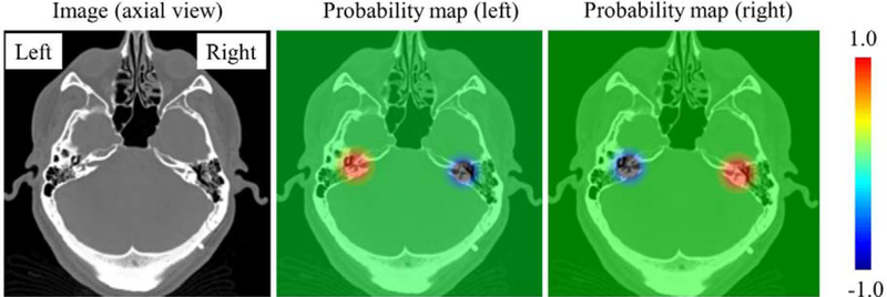
Results we obtain with this approach are not satisfactory because it leads to a large number of false positives. We observe that the response map associated with one inner ear can have a very high response at the location of the other ear, possibly due to their similar intensity characteristics. In turn, this leads to a substantial number of wrong detections. To solve this problem, we incorporate a false positive suppression strategy during training. Specifically, for the probability map associated with one ear, if the ear on the other side of the head is included in the image, we force the values around this second inner ear to be negative rather than zero to penalize the detection of the erroneous ear. The negative values that are used are the same Gaussian-distributed values that are used for the correct ear but centered on the incorrect ear and multiplied by minus one. By penalizing the network in such a way, we effectively suppress the number of false positives. Fig. 5 shows one slice in a training image that contains two ears and the associated two probability maps, one for the left and the other for the right ear.

Fig. 5.

The probability maps designed to suppress false positives. From left to right, one slice in the training volume, the left probability map, and the right probability map. (For interpretation of the heat maps, please refer to the online version)

Even though the aforementioned method suppresses false positives caused by the contralateral ear, other false positives remain present at some random positions, e.g., the location of the CI transmitters in some post-operative CTs. To alleviate this problem, we capture the spatial relationship between inner ear pairs using a low-dimension shape model and use this a-priori information to further evaluate the plausibility of the detected inner ear pairs in a post-processing step. More details on this earlier approach that we call HeadLocNet-1 (Head CT Localization Network for 1 landmark) can be found in (Zhang et al. 2018b).

3.2. HeadLocNet-MC: Co-learning Image Volume Classification and Landmark Set Localization

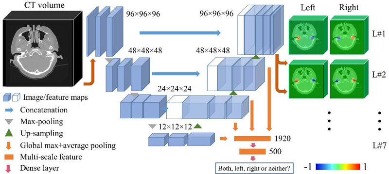
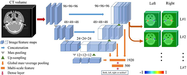
As discussed previously, to automate our IGCIP process we need to estimate transformations that are used to initialize intensity-based registration algorithms. The approach we follow in this work is to localize a set of landmarks that are used to compute a rigid-body transformation using a point-based registration method. To do so, we extend the solution we have presented above and we propose a network architecture that can co-task image content classification and landmark set detection. Based on the previous network architecture, we first set the number of output channels to 14, i.e., 7 for each side of the head. Second, instead of simply using the output probability maps as indicators of whether or not an inner ear exists, we add a classification branch to the main path of the 3D U-Net. As is shown in Fig. 6, in the upsampling stage of the 3D U-Net, we use the feature maps as input to the classifier. Because the dimensionality of the feature maps is large, which could cause overfitting, we use global pooling operations to perform dimensionality reduction. For each feature map, we use a global max pooling and a global average pooling, reducing its dimensionality from M³ with M =12, 24, 48 or 96 to 2. The hierarchical features we extract from the multi-level feature maps are used as input to a classifier. The classifier is designed to be a fully-connected network with one hidden layer (500 units). The number of output units is 4. We thus use a richer feature set than the one we used previously to determine what ear(s) are present in the image if any. As will be shown this improves performance. To train the network to recognize the content of the image, we use the categorical cross entropy between the ground truth and the prediction as the loss function.

Fig. 6.

The HeadLocNet-MC architecture. (For interpretation of the heat maps, please refer to the online version)

We also modify the probability map regression loss function we used previously. In addition to assigning larger weights to non-zero entries in the ground truth probability maps, we penalize more entries for which the predicted values deviate too much from the ground truth maps. That is to say, in one training iteration, for each sample we define the loss as follows:

$$loss(\mathit{P},\widehat{\mathit{P}})=\frac{1}{N^{3}L}\sum _{l=1}^L\sum _{k=1}^N\sum _{j=1}^N\sum _{i=1}^N{w}_{i,j,k,l}{(P_{i,j,k,l}-{\widehat{P}}_{i,j,k,l})}^2.$$ (4)

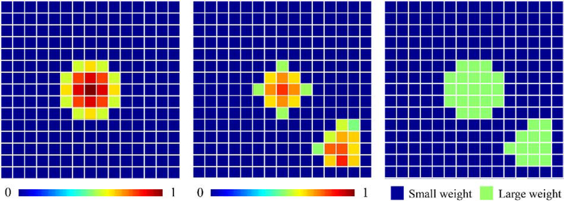
Here, L is the number of landmarks, N = 96 is the dimensionality of each probability map. P and $\widehat{\mathit{P}}$ are the ground truth probability maps and the predicted probability maps, respectively. w_i,j,k,l is set to a large value if $|P_{i,j,k,l}-{\widehat{P}}_{i,j,k,l}|>\mathrm{\Delta }$ (Δ is empirically set to 0.2) or if |P_i,j,k,l| > 0. Otherwise, it is set to a small value. The large value and small value are set to w_nonzero and w_zero introduced in Section 3.3, respectively. By doing so, we can penalize more the regions in which false negatives and false positives happen.

The loss function of the whole network is an unweighted sum of the classification loss, i.e., the categorical cross entropy and the regression loss in equation (4). An illustration of our weighting scheme in 2D is shown in Fig. 7. We call this new network HeadLocNet-MC (Head CT Localization Network for Multiple landmarks with Classification). Since we design the classification branch to directly determine the included side of the head, we do not use in HeadLocNet-MC the shape-based post-processing step which is used in HeadLocNet-1.

Fig. 7.

An example of the probability map ground truth (left), predicted probability map at one iteration (middle) and the generated weight matrix (right) in HeadLocNet-MC. (For interpretation of the heat maps, please refer to the online version)

4. Experimental Settings

Image preprocessing, including resampling, cropping, padding and intensity normalization is done using MATLAB. We train the neural networks using stochastic gradient descent (SGD) with 0.9 momentum and an initial learning rate of 0.0001. The batch size is set to 1. The code is written in Keras developed by Chollet (Chollet 2015) and runs on an Nvidia Titan X GPU. We train each model for 30 epochs. A forward propagation to process one image using the model takes ~1.4 seconds on average. We also integrate this method (written in python) into our CI programming software package. The total time to process one subject’s image including the overhead to load Keras and the trained weights from the disk, and the forward propagation is about 15s.

5. Results

5.1. Results obtained with HeadLocNet-1

To facilitate comparison with earlier work, results obtained with HeadLocNet-1are summarized in this section. As shown in the top row of Table 2 and the left panel of Table 3, this approach achieved an overall classification accuracy of 98.6% with the shape-based false positive post-processing step. This is substantially higher than the 96% obtained with the slice-wise network that was proposed in (Zhang et al. 2018a). For the test CT volumes that are correctly classified, we calculate the landmark localization error and report it in the lower part of Table 2. As mentioned earlier, the landmark that was used in this study is landmark #5, which corresponds roughly to the center of the labyrinth, and the localization error is computed as the distance between the manually labeled inner ear position and the automatic localization.

Table 2.

Error rates and localization error using obtained with HeadLocNet-1.

	CTs classified by presence of CI		CTs classified by scanner		Overall
Classification error rate	w/ CI	w/o CI	convCT	lCT
	0.77%	1.53%	1.50%	1.09%	1.41%
Localization error (in mm)	2.32±2.34	2.48±2.35	2.41±1.13	2.57±4.49	2.45±2.35

Table 3.

Confusion matrices for each category obtained with HeadLocNet-1, HeadLocNet-M and HeadLocNet-MC

	HeadLocNet-1				HeadLocNet-M				HeadLocNet-MC
Truth╲Predict	Both	Left	Right	Neither	Both	Left	Right	Neither	Both	Left	Right	Neither
Both	618	5	1	1	613	4	5	3	621	2	0	2
Left	0	619	2	4	1	613	0	11	1	623	1	0
Right	0	4	613	8	2	1	616	6	5	1	619	0
Neither	1	4	5	611	0	0	2	619	1	0	0	620

5.2. Results obtained with HeadLocNet-MC

We evaluate the classification performance of our trained HeadLocNet-MC model presented in Section 3.3 on the same test set we use to evaluate the HeadLocNet-1 solution. The classification error rate is 0.52%, showing a further improvement over the 1.41%, produced by HeadLocNet-1.

The two main differences between HeadLocNet-MC and HeadLocNet-1 are: (1) HeadLocNet-MC uses multi-scale feature maps in the intermediate layers of the neural network instead of only relying on the final output to classify images and (2) it uses information about 7 landmarks rather than one for supervision. To evaluate each factor’s contribution to the classification performance improvement, we perform an ablation study: we train another model which is almost identical to the proposed HeadLocNet-MC except that it does not have the classification branch. We call this version HeadLocNet-M. As we do in HeadLocNet-1, in HeadLocNet-M, we threshold the maximum of each probability map on one side of the head to determine the presence of the inner ear using a majority voting strategy. Specifically, we predict that an inner ear exists if and only if at least 4 landmarks are detected around it (shape-based false positive elimination is not applied in this case since the number of landmarks exceeds two). With this approach we achieve a classification error rate of 1.41%, which is the same as what is obtained with HeadLocNet-1. Confusion matrices in Table 3 show that HeadLocNet-1 and HeadLocNet-M behave similarly, and that HeadLocNet-MC outperforms these in all four categories, i.e., both, left, right, and neither. This indicates that it is the utilization of multi-scale features in the intermediate layers rather than the additional landmarks’ supervision information that contributes to the improvement. Fig. 8 illustrates the effectiveness of the HeadLocNet-MC’s classification branch. It shows the heat maps generated by HeadLocNet-M and HeadLocNet-MC for one test image for which HeadLocNet-M fails but HeadLocNet-MC succeeds in classification. In this particular case, the image elicits weak heat maps from both HeadLocNet-M and HeadLocNet-MC (for HeadLocNet-M, heat map #3 reaches 0.5 but all others do not). As a consequence, the detection rule used in HeadLocNet-M, i.e., four landmarks above 0.5, is not triggered. HeadLocNet-MC is however able to assign the image to the correct class thanks to the rich features used in its classification branch.

Fig. 8.

The seven heat maps of a right ear generated by HeadLocNet-M and HeadLocNet-MC using an image that HeadLocNet-M fails but HeadLocNet-MC succeeds in classifying. (For interpretation of the heat maps, please refer to the online version)

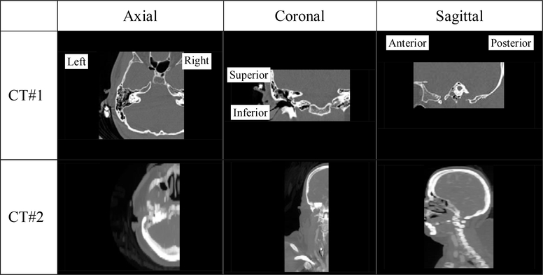
We check the cases that are incorrectly classified by HeadLocNet-MC and show two examples in Fig. 9. The first case had been manually labeled as “both inner ears” because both cochlea are present. However, the right side of the head is only partially covered and most landmarks surrounding the right cochlea are not included. The network labels it as a “left ear” image. For the second image, the wrong prediction of “both ears” is likely due to an abnormally large FOV. It is worth noting that even though the right ear of CT#1 and the left ear of CT#2 are included, they could not be used for IGCIP because: (1) in CT#1 the portion of the right ear is so small that image segmentation algorithms cannot be applied. (2) The quality of CT#2 is too low to get meaningful cochlear segmentation. Visual inspection of other failure cases also reveals that they are caused by unusual acquisitions.

Fig. 9.

Two examples of wrong predictions

We then evaluate the landmark localization performance of HeadLocNet-MC. To do so, we use the maximum of each probability map as our prediction of the landmark position. We show the overall localization error averaged across all 7 landmarks in Table 4. To test the effect of simultaneous localization on localization accuracy we compare the localization error of each individual landmark obtained with HeadLocNet-1 and HeadLocNet-MC. The HeadLocNet-1 results for Landmark #5 are readily available because this landmark has been used to produce the results presented earlier. To produce results for the remaining 6 landmarks we train another 6 HeadLocNet-1 models, one for each landmark. For each of these we compute the localization error and the classification error. We also compute the localization errors for HeadLocNet-M for each landmark. The classification error of the seven HeadLocNet-1 models is shown in Table 5 and the localization errors are all shown in Table 6. From data presented in Tables 5 and 6, we can conclude that (1) in terms of classification, HeadLocNet-MC has substantially lower error rate than HeadLocNet-1 trained on each of the seven landmarks and that the results obtained with HeadLocNet-1 are sensitive to the choice of landmark. Interestingly, landmark #5 that was used in our earlier work is the one for which the difference is the smallest. (2) HeadLocNet-MC produces better localization results than HeadLocNet-1 for four landmarks (#2, #3, #4, #6) and slightly worse results than HeadLocNet-1 for three landmarks (#1, #5, #7). Paired t-tests show that there is a statistically significant difference (p < 0.01) between the two methods for landmark #2, #3, #4, #6 and #7. There is no statistically significance (p > 0.01) between the two methods for landmark #1 and #5. Overall, we can conclude that HeadLocNet-MC produces better or equivalent results than HeadLocNet-1 for landmark localization. (3) HeadLocNet-M has a slightly better localization accuracy than HeadLocNet-MC. The differences are found statistically significant for landmark #1, #3, #4, #5 and #6 and are not statistically significant for landmark #2 and #7. The overall localization error of HeadLocNet-M averaged across all 7 landmarks is 3.11mm, only slightly but significantly different than the 3.45mm localization error obtained with HeadLocNet-MC. Thus, co-learning classification and localization does not improve localization while co-learning the location of the landmarks tends to improve the results.

Table 4.

Error rates of HeadLocNet-M and HeadLocNet-MC, and landmark set localization error of HeadLocNet-MC

Classification error rate
	CTs Classified by presence of CI		CTs Classified by scanner		Overall
	w/ CI	w/o CI	convCT	lCT
HeadLocNet-M	1.03%	1.47%	1.65%	0.54%	1.41%
HeadLocNet-MC	0.26%	0.57%	0.67%	0	0.52%
Localization error (in mm)
HeadLocNet-MC	3.31±1.32	3.49±2.10	3.45±1.96	3.48±1.98	3.45±1.97

Table 5.

Classification error rate for networks trained to detect one single landmark. “Ldmk” is used for “Landmark”.

Network╲Ldmk	#1	#2	#3	#4	#5	#6	#7
HeadLocNet-1	2.36%	4.57%	7.81%	3.45%	1.41%	8.49%	9.05%

Table 6.

Localization errors of each landmark, generated using HeadLocNet-1, HeadLocNet-M and HeadLocNet-MC. “Ldmk” is used for “Landmark”.

Network╲Ldmk	#1	#2	#3	#4	#5	#6	#7
Head-LocNet-1	3.66±3.05	3.74±5.77	3.81±6.70	3.42±4.48	2.45±2.35	4.70±9.97	4.80±5.39
HeadLocNet-M	3.58±4.77	3.11±4.30	2.71±3.51	2.45±2.32	2.27±1.76	3.10±2.62	4.54±5.43
HeadLocNet-MC	3.78±1.83	3.22±2.68	3.24±1.98	2.94±1.40	2.58±1.25	3.36±3.49	4.82±5.70

As noticed above, Tables 5 and 6 show the sensitivity of the classification and localization results obtained with HeadLocNet–1 to the landmark selection. This is caused by both the location of the landmarks and the ease with which they can be localized manually to generate the training set. Landmarks #3, #6, #7 can be close to the border of the images when volumes cover only part of the head. When this is the case, border effects reduce the response of the network and, as a result, the maximum response falls below the detection threshold. Landmark #4 is selected as the center of an ossicle and Landmark #5 is selected as the center of the labyrinth. Both structures are very small and can be easily distinguished from their surrounding structures. The other five landmarks are more difficult to localize: Landmark #1 is selected as the center of the temporal bone and the trabecular bones surrounding it has nearly random patterns. Landmark #2 is selected as a point in the ear canal which is homogeneously filled with air. Landmarks #3, #6 and #7 are not as distinguishable as #4 and #5 as can be appreciated from Fig. 4. Localization results obtained with all networks are lower for landmarks #4 and #5 than for the other landmarks.

6. Conclusions and Discussions

In this article, we present a method for the localization of multiple landmarks in head CTs and for the automatic documentation of their content. We focus on the detection of landmarks around the ear and on documenting whether the image volume contains two ears, one ear, or neither. Although other methods have been proposed for the detection of landmarks in CT images, at the time of writing, we do not know of any other work addressing this particular problem and it is a critical step toward the large scale deployment of our IGCIP technique. We begin by describing the work we have presented in (Zhang et al. 2018b). We call this early solution HeadLocNet-1. It relies on a 3D U-Net with false positive suppression and a shape-based constraint. This deep-learning solution outperforms earlier methods we have proposed for content labeling of head CT images (Zhang et al. 2018a) and for landmark localization (Zhang et al. 2017a). We expand our HeadLocNet-1 solution to produce a new network architecture which we call HeadLocNet-MC. This new solution includes a one-hidden-layer classification branch that uses hierarchical features from the intermediate layers of 3D U-Net as input. The overall network is therefore trained using a sum of the classification loss, i.e., the cross entropy, and the regression loss. We test this network on a data set that, before augmentation, contains 795 volume acquired from 153 subjects. We show that on this data set HeadLocNet-MC (1) works in an end-to-end fashion, with no need for post-processing, (2) is able to document the content of head CTs better than HeadLocNet-1 and reach a high classification accuracy of 99.5%, and (3) is able to robustly localize the 7 landmarks (14 in total for both sides) in one pass with no loss of accuracy compared with HeadLocNet-1. As discussed in the introduction section, a number of methods have been proposed to detect landmarks in medical images. A side-by-side comparison of these methods is difficult and would be beyond the scope of this article. Nevertheless, a semi-quantitative comparison is possible using published results. To that end we rely on data compiled recently by (Ghesu et al. 2019) to compare the method they propose to detect eight landmarks in mostly abdominal pelvic CT images to several other methods that are considered to be state of the art. In their article, they show that their method outperforms others for most of these landmarks. To perform this analysis we rely on results they report for six landmarks: (1) the right front corner of the hip bone, (2) the left front corner of the hip bone, (3–5) three vessel bifurcations between the aortic arch and the subclavian artery, the left common carotid artery, and the brachiocephalic artery, and (6) the bronchial bifurcation. We exclude two other landmarks, i.e., the right and left kidney centers because these are non-rigid organs and larger structures, which makes localizing their center more difficult both manually and automatically. Indeed, the automatic localization error they report for these two landmarks (6.72mm and 6.89mm) is much higher than the error reported for the other landmarks. We note that their algorithm operates on 2×2×2 mm³ voxels and ours on 2.25×2.25×2.25mm³ voxels, making the comparison possible but their annotated data set is substantially larger than ours, ranging from 552 annotations for the front corner of the left hip bone to 1054 annotations for the front corner of the right hip-bone. Table 7 compares localization errors for these six landmarks to the localization errors we obtain on our seven landmarks.

Table 7.

A comparison of localization errors achieved with the method proposed by Ghesu et al. 2019 and with our method. All errors are in mm.

Landmark #	Ghesu et al. 2019	Ours
1	2.80±1.46	3.78±1.83
2	3.07±2.14	3.22±2.68
3	3.89±1.95	3.24±1.98
4	3.71±2.01	2.94±1.40
5	3.09±1.50	2.58±1.25
6	3.35±1.77	3.36±3.49
7		4.82±5.70
Mean of means	3.32	3.45

This table shows that despite differences in organs, data sets, landmark visibility, and ease of localization of these landmarks, the results we have obtained are comparable to those reported by (Ghesu et al. 2019) with overall means that are very close to each other. It is possible that their method performs as well as or better than ours on our application, but this cannot be definitely assessed without retraining their network on our data. Similarly, we have not tested the applicability of our approach for the detection of other landmarks on other body parts and can therefore not speculate on the generalizability of our technique. We note however that the purpose of our work is not to come up with the absolute best landmark localization error but to come up with a solution that both classifies the images and localizes the landmarks. We are in fact willing to take a little hit on the localization accuracy, i.e., select HeadLocNet-MC rather than HeadLocNet-M that leads to the best localization accuracy, to achieve a better classification rate because in our application landmarks are used to initialize an intensity-based registration algorithm that is robust to small difference in the starting point.

The work presented in this article is a significant step toward full automation of our IGCIP process, thus facilitating its clinical use and deployment. Inspection of failure cases reveals that they are often caused by unusual acquisitions. Improving the network performance even further to bring our processes to full automation will necessitate adding a mechanism to detect abnormal images.

HIGHLIGHTS.

• A deep volume classification and voxel-wise regression network to process whole 3D CT volumes.

• An adaptively adjusted loss function for voxel-wise regression.

• It has substantially better classification performance compared with the previous conference paper and the new features in it are extensively studied.

References

- Breiman Leo. 2001. “Random Forests.” Machine Learning 45(1): 5–32. François Chollet. 2015. “Keras.” [Google Scholar]
- Çiçek Özgün et al. 2016. “3D U-Net: Learning Dense Volumetric Segmentation from Sparse Annotation.” In International Conference on Medical Image Computing and Computer-Assisted Intervention, 424–32. 10.1007/978-3-319-46723-8_49 [DOI] [Google Scholar]
- Criminisi A et al. 2013. “Regression Forests for Efficient Anatomy Detection and Localization in Computed Tomography Scans.” Medical Image Analysis 17(8): 1293–1303. 10.1016/j.media.2013.01.001. [DOI] [PubMed] [Google Scholar]
- Donner Rene, Menze Bjoern H., Bischof Horst, and Langs Georg. 2013. “Global Localization of 3D Anatomical Structures by Pre-Filtered Hough Forests and Discrete Optimization.” Medical Image Analysis 17(8): 1304–14. 10.1016/j.media.2013.02.004 [DOI] [PMC free article] [PubMed] [Google Scholar]
- Ebner Thomas et al. 2014. “Towards Automatic Bone Age Estimation from MRI: Localization of 3D Anatomical Landmarks.” In Medical Image Computing and Computer Assisted Intervention, 10.1007/978-3-319-10470-6_53 [DOI] [PubMed] [Google Scholar]
- Ghesu Florin C et al. 2019. “Multi-Scale Deep Reinforcement Learning for Real-Time 3D-Landmark Detection in CT Scans.” IEEE Transactions on Pattern Analysis and Machine Intelligence 41(1): 176–89. 10.1109/TPAMI.2017.2782687 [DOI] [PubMed] [Google Scholar]
- Ghesu Florin C. et al. 2018. “Towards Intelligent Robust Detection of Anatomical Structures in Incomplete Volumetric Data.” Medical Image Analysis 48: 203–13. 10.1016/j.media.2018.06.007. [DOI] [PubMed] [Google Scholar]
- Han Dong et al. 2015. “Robust Anatomical Landmark Detection with Application to MR Brain Image Registration.” Computerized Medical Imaging and Graphics 46: 277–90. 10.1016/j.compmedimag.2015.09.002.. [DOI] [PMC free article] [PubMed] [Google Scholar]
- Lindner Claudia et al. 2016. “Fully Automatic System for Accurate Localisation and Analysis of Cephalometric Landmarks in Lateral Cephalograms.” Scientific Reports 6(September). 10.1038/srep33581. [DOI] [PMC free article] [PubMed] [Google Scholar]
- Liu Mingxia, Zhang Jun, Adeli Ehsan, and Shen Dinggang. 2018. “Landmark-Based Deep Multi-Instance Learning for Brain Disease Diagnosis.” Medical Image Analysis 43: 157–68. 10.1016/j.media.2017.10.005. [DOI] [PMC free article] [PubMed] [Google Scholar]
- Maicas Gabriel et al. 2017. “Deep Reinforcement Learning for Active Breast Lesion Detection from DCE-MRI.” In Medical Image Computing and Computer-Assisted Intervention, 665–73. 10.1007/978-3-319-66179-7_76 [DOI] [Google Scholar]
- Mehta Sachin et al. 2018. “Y-Net: Joint Segmentation and Classification for Diagnosis of Breast Biopsy Images.” In Medical Image Computing and Computer Assisted Intervention,, 893–901. 10.1007/978-3-030-00934-2_99 [DOI] [Google Scholar]
- NIDCD. 2011. “Fact Sheet: Cochlear Implants.” NIH Publication No. 11–4798: 1–4. https://www.nidcd.nih.gov/health/hearing/pages/coch.aspx.
- Noble Jack H et al. 2016. “Initial Results With Image-Guided Cochlear Implant Programming in Children.” Otology & Neurotology 37(2): e63–69. 10.1097/MAO.0000000000000909 [DOI] [PMC free article] [PubMed] [Google Scholar]
- Noble Jack H. et al. 2014. “Clinical Evaluation of an Image-Guided Cochlear Implant Programming Strategy.” Audiology and Neurotology 19(6): 400–411. 10.1159/000365273 [DOI] [PMC free article] [PubMed] [Google Scholar]
- Noble Jack H., Labadie Robert F., Gifford Renea H., and Dawant Benoit M. 2013. “Image-Guidance Enables New Methods for Customizing Cochlear Implant Stimulation Strategies.” IEEE Transactions on Neural Systems and Rehabilitation Engineering 21(5): 820–29. 10.1109/TNSRE.2013.2253333 [DOI] [PMC free article] [PubMed] [Google Scholar]
- Noble Jack H., Labadie Robert F., Majdani Omid, and Dawant Benoit M. 2011. “Automatic Segmentation of Intracochlear Anatomy in Conventional CT.” IEEE Transactions on Biomedical Engineering 58(9): 2625–32. 10.1109/TBME.2011.2160262 [DOI] [PMC free article] [PubMed] [Google Scholar]
- Payer Christian, Stern Darko, Bischof Horst, and Urschler Martin. 2016. “Regressing Heatmaps for Multiple Landmark Localization Using CNNs.” In International Conference on Medical Image Computing and Computer-Assisted Intervention, 230–38. 10.1007/978-3-319-46723-8_27 [DOI] [Google Scholar]
- Rohr Karl. 2001. 21 Springer Science & Business Media Landmark-Based Image Analysis: Using Geometric and Intensity Models. [Google Scholar]
- Xu Zhoubing et al. 2018. “Less Is More: Simultaneous View Classification and Landmark Detection for Abdominal Ultrasound Images.” In Medical Image Computing and Computer-Assisted Intervention, Springer International Publishing, 711–19. 10.1007/978-3-030-00934-2_79 [DOI] [Google Scholar]
- Yang Dong et al. 2017. “Automatic Vertebra Labeling in Large-Scale 3D CT Using Deep Image-to-Image Network with Message Passing and Sparsity Regularization.” In Information Processing in Medical Imaging, 633–44. 10.1007/978-3-319-59050-9_50 [DOI] [Google Scholar]
- Zhang Dongqing, Liu Yuan, Noble Jack H., and Dawant Benoit M. 2017a. “Localizing Landmark Sets in Head CTs Using Random Forests and a Heuristic Search Algorithm for Registration Initialization.” Journal of Medical Imaging 4(4): 44007. [DOI] [PMC free article] [PubMed] [Google Scholar]
- Zhang Dongqing, Noble Jack H., and Dawant Benoit M. 2018a. “Automatic Detection of the Inner Ears in Head CT Images Using Deep Convolutional Neural Networks.” In SPIE Conference on Medical Imaging, 10574. [DOI] [PMC free article] [PubMed] [Google Scholar]
- Zhang Dongqing, Wang Jianing, Noble Jack H., and Dawant Benoit M. 2018b. “Accurate Detection of Inner Ears in Head CTs Using a Deep Volume-to-Volume Regression Network with False Positive Suppression and a Shape-Based Constraint.” In Medical Image Computing and Computer-Assisted Intervention, Springer, Cham, 703–11. 10.1007/978-3-030-00937-3_80 [DOI] [PMC free article] [PubMed] [Google Scholar]
- Zhang Jun et al. 2016. “Detecting Anatomical Landmarks for Fast Alzheimer’s Disease Diagnosis.” IEEE Transactions on Medical Imaging 35(12): 2524–33. 10.1109/TMI.2016.2582386 [DOI] [PMC free article] [PubMed] [Google Scholar]
- Zhang Jun, Liu Mingxia, and Shen Dinggang. 2017b. “Detecting Anatomical Landmarks from Limited Medical Imaging Data Using Two-Stage Task-Oriented Deep Neural Networks.” IEEE Transactions on Image Processing 26(10): 4753–64. 10.1109/TIP.2017.2721106 [DOI] [PMC free article] [PubMed] [Google Scholar]
- Zhao Yiyuan et al. 2019. “Automatic Graph-Based Method for Localization of Cochlear Implant Electrode Arrays in Clinical CT with Sub-Voxel Accuracy.” Medical Image Analysis 52: 1–12. 10.1016/j.media.2018.11.005 [DOI] [PMC free article] [PubMed] [Google Scholar]
- Zhao Yiyuan, Dawant Benoit M, Labadie Robert F, and Noble Jack H. 2018. “Automatic Localization of Closely-Spaced Cochlear Implant Electrode Arrays in Clinical CTs.” Medical Physics 45(11): 5030–40. 10.1002/mp.13185 [DOI] [PMC free article] [PubMed] [Google Scholar]
- Zheng Yefeng et al. 2012. “Automatic Aorta Segmentation and Valve Landmark Detection in C-Arm CT for Transcatheter Aortic Valve Implantation.” IEEE Transactions on Medical Imaging 31(12): 2307–21. 10.1109/TMI.2012.2216541 [DOI] [PubMed] [Google Scholar]