Abstract
Pneumonia is responsible for high infant morbidity and mortality. This disease affects the small air sacs (alveoli) in the lung and requires prompt diagnosis and appropriate treatment. Chest X-rays are one of the most common tests used to detect pneumonia. In this work, we propose a real-time Internet of Things (IoT) system to detect pneumonia in chest X-ray images. The dataset used has 6000 chest X-ray images of children, and three medical specialists performed the validations. In this work, twelve different architectures of Convolutional Neural Networks (CNNs) trained on ImageNet were adapted to operate as the resource extractors. Subsequently, the CNNs were combined with consolidated learning methods, such as k-Nearest Neighbor (kNN), Naive Bayes, Random Forest, Multilayer Perceptron (MLP), and Support Vector Machine (SVM). The results showed that the VGG19 architecture with the SVM classifier using the RBF kernel was the best model to detect pneumonia in these chest radiographs. This combination reached 96.47%, 96.46%, and 96.46% for Accuracy, F1 score, and Precision values, respectively. Compared to other works in the literature, the proposed approach had better results for the metrics used. These results show that this approach for the detection of pneumonia in children using a real-time IoT system is efficient and is, therefore, a potential tool to aid in medical diagnoses. This approach will allow specialists to obtain faster and more accurate results and thus provide the appropriate treatment.
Keywords: Pneumonia detection, Real-time IoT system, Transfer learning, Convolutional neural networks
Introduction
Childhood respiratory diseases are a severe public health problem in many countries, especially in Southeast Asia and sub-Saharan Africa. Data from the World Health Organization (WHO) reveals that pneumonia is responsible for high morbidity and mortality in children under 5 years old. About 15% of all deaths in this age group are due to this disease.
Magnetic resonance imaging (MRI), chest X-ray (CXR), and computed tomography (CT) are imaging tests used to diagnose pneumonia [21]. CXR is the most common method to detect pneumonia worldwide due to its low cost, speed, and availability. In addition to pneumonia, radiography can be used to diagnose other pathologies, such as the detection of fractures [23, 31, 33], cavities [16], and tumors [32].
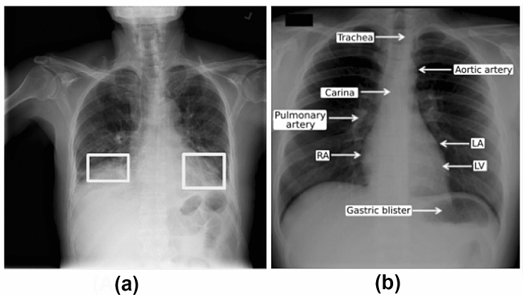
Pneumonia usually manifests itself as an area or areas of greater opacification in chest radiographs. Figure 1a shows a CXR of a patient with pneumonia. The opaque regions in this figure confirm the diagnosis of pneumonia. Figure 1 also shows other anatomical structures, such as the heart, bones, and blood vessels, as shown in Fig. 1b.
Fig. 1.
a Example of pulmonary opacities; b Normal chest radiography showing the main identifiable anatomical structures (LA left atrium, LV left ventricle, AD right atrium)
Detecting pneumonia on CXR is a challenge even for experienced professionals as other lung abnormalities, such as lung cancer and excess fluid, can show similar opacities. In addition to such lung abnormalities, the expert’s interpretation can also be influenced by the position of the patient and level of inspiration at the moment of the examination.
In addition to the factors inherent to the examination, other factors at the moment of analysis and interpretation can contribute to an erroneous diagnosis: (1) subjectivity and experience of the professional, (2) work fatigue due to repetitive actions, and (3) lighting levels in the consultation room.
Given this scenario, the detection of pneumonia in children from the conventional analysis of CXR images is time-consuming and subjective. These factors cause a delay in both the diagnosis and treatment. Therefore, there is a need for a reliable system capable of overcoming such difficulties so that the professional can diagnose and refer the patient for treatment in real-time and with greater assurance.
Artificial intelligence techniques are multi-purpose procedures that are mainly dedicated to classification, prediction, and grouping [26]. Due to the significant impact on morbidity in children, pneumonia is a disease that requires a rapid diagnosis and appropriate treatment. Computerized diagnostics (CAD) using the Internet of Things technology have gained space in the medical community. These systems are justified due to their fast response and increased accuracy in medical diagnoses. These factors are important, especially in regions where clinical conditions are precarious. Real-time IoT systems to assist doctors have been proven to be effective. They have been successful in detecting and in analyzing cranial effusions in computed tomography images [5, 28], and to classify electrocardiograms (ECG) [10], among others [24].
According to the United Nations International Children’s Emergency Fund (UNICEF), one way to obtain better results in the clinical treatment of pneumonia in children is to carry out real-time diagnoses. Thus, the use of a real-time IoT system, which doctors can use anywhere, would guarantee that more people would be diagnosed rapidly and without prejudice to subjective and structural factors.
The emergence of Convolutional Neural Networks (CNN) and the recent advances in computational power have boosted progress in using computational methods to assist specialists in analyzing clinical diseases. One of the main factors for the high performance of CNNs is the ability of neural networks to learn high-level abstractions from raw data through transfer learning techniques.
Advances in the use of CNN’s have improved specialists’ performance in the modalities of segmenting anatomical structures [6, 9, 11, 22], and of classifying and detecting diseases [5]. Several important approaches to detect pneumonia have been proposed by Ayan and Ünver [1], Chouhan et al. [4], and Kermany et al. [18].
The approach proposed in this work has potential because it integrates proven methods, which have given excellent results with low computational costs, and allows their implementation in an IoT system with free access. The proposed system has accuracy superior to or equal to the methods already proposed and has stability, computational efficiency, accessibility, and overcomes the socio-economic issues.
Considering the context of lung problems, the difficulty in diagnosing pneumonia from CXR images, and the motivation for the concept of the Internet of Things (IoT) and Transfer Learning, this article proposes an automatic, fast, and accessible system that assists doctors in the diagnosis of pneumonia. This system uses and complements techniques already consolidated in the literature from new combinations of CNNs with machine learning classifiers, all in a real-time IoT system.
The main contributions of this work are listed below:
The analysis of twelve CNNs as feature extractors combined with seven classic classifiers to maximize the performance of a system aimed at medical assistance in diagnosing pneumonia.
A method consolidated in a real-time IoT system for clinical predictions in the medical field.
An interactive and easy-to-use system to assist specialists in the diagnosis of pneumonia in children.
The remainder of this article is organized as follows: Sect. 2 presents a brief literature review of studies for the diagnosis of pneumonia; Sect. 3 presents the methodology of the proposed approach; Sect. 4 presents the results and their respective discussions, while Sect. 5 presents the main conclusions and possible future work.
Related works
In recent years, significant progress has been made in developing antibiotics, vaccines, and pneumonia treatments. However, this disease remains a public health problem. Consequently, research using computational methods capable of segmenting, detecting, and classifying pneumonia to support the medical community is recurrent in the literature [8].
Motivated by the satisfactory results with CNN in the diagnosis of other diseases [2, 19], the primary methods for the determination of pneumonia have also explored the use of CNNs.
An extensive literature search showed that the most satisfactory results in the diagnosis of pneumonia were developed in the works of Ayan and Ünver [1], Chouhan et al. [4], and Kermany et al. [18]. All authors used CNN in their research.
Ayan and Ünver [1] used the Xception and VGG16 architectures with transfer learning and fine-tuning. They changed the Xception model freezing the last 10 layers of the network, adding two fully connected layers and a two-way output layer with a SoftMax activation function. The motivation presented is that the greatest generalization capacity is in the first layers of the network. In the VGG16 architecture, the final eight layers were frozen, and there were changes to the fully connected layers. Thus, the work obtained a test time per image equivalent to 16 and 20 ms for the VGG16 and Xception networks, respectively.
Chouhan et al. [4] used the AlexNet, DenseNet121, InceptionV3, ResNet18 and GoogLeNet architectures. The diagnosis is based on a classifying committee composed of CNN models. Each model was part of the hypothesis of inducing the diagnosis through a vote. The majority vote, in their work, was used to combine the results of the classifiers. Therefore, the diagnosis corresponds to the class that achieved the highest number of votes. This approach obtained an average test time per image equivalent to 161 ms for the model. In addition, they achieved high percentages of classification for X-ray images. This shows that deep networks are an area of research that can help diagnose pneumonia. In our approach, eight architectures are evaluated more than in the work of Chouhan et al. [4]. Furthermore, we adopt traditional classifiers to reduce the classifying computational cost.
In both works, data augmentation was performed with variations of displacement, zoom, inversion, and rotation at angles of , Random Horizontal Flip, and Random Resized Crop, for example.
Kermany et al. [18] developed a method for diagnosing optical coherence tomography (OCT). The authors took advantage of the method and applied it to the diagnosis of pneumonia in children. They focused on proving the generalization of the proposed system. The work did not make comparisons with other similar methods or demonstrate the computational costs to reach their results.
Despite having obtained satisfactory results, all the approaches above generated their results with only 624 images. This corresponds to about half the number of images tested in our proposed work. The results above would be more reliable if they were obtained with a larger number of images and standard deviations.
Another prominent approach was that of Rahimzadeh et al. [27], who proposed to detect COVID-19, pneumonia, and normal from X-ray examinations. Rahimzadeh et al. proposed a network based on the concatenation of the Xception and ResNet50V2 networks. Due to the imbalance in the number of samples, the network’s training was divided into eight stages with equivalent numbers of samples. The results obtained show a disparity between the classes and a limitation in the generalization of the system to new samples of COVID-19. The method uses the same COVID-19 images at each new training stage and only 31 images for validation. The reliability of the results would be greater with data augmentation, standard deviations, and a demonstration of the computational costs.
Table 1 shows a chronological summary of the works to be compared with the proposed approach. Table 1 is organized, showing the approach, the main highlights, the disadvantages, and the Integration, if any, into an IoT system.
Table 1.
Chronological summary of the works to be compared with the proposed approach. The table shows the approach, the main highlights, and disadvantages. In addition, if any of these works related their application to an IoT system
| Works | Approach | Advantages | Disadvantages | IoT system |
|---|---|---|---|---|
| Ayan and Ünver [1] | Transfer Learning + Fine-tuning | The authors used data augmentation | The number of images for training is 8.3 more than those used for testing | No |
| Kermany et al. [18] | Transfer learning | The authors effectively classified the images for macular degeneration and diabetic retinopathy. Also, it obtained satisfactory results for pneumonia, although this is not the focus of the article | The number of images for training is 8.3 more than those used for testing | No |
| Rahimzadeh et al. [27] | Concatenation of Xception and ResNet50V2 | Concatenation of Xception and ResNet50V2 | The authors use images from COVID-19. Consequently, classes become unbalanced | No |
| Chouhan et al. [4] | Five different pre-trained architectures + majority vote classification | The results indicate that deep learning methods can be used to simplify the pneumonia diagnosis process | The authors affirm the need to evaluate the most sophisticated deep networks. At work, only five nets were used | No |
Some companies have developed devices capable of assisting doctors in diagnosing pneumonia. However, to acquire these systems, it is necessary to have high purchasing power to pay for the license. Therefore, it is not accessible to professionals at the beginning of their careers or hospitals with low purchasing power.
The proposed work uses CNN and transfer learning combined with classic classifiers in an IoT system accessible to all. This system’s characteristics enable high performance, low computational costs, and overcomes the financial problems mentioned. An IoT system makes it possible to diagnose and identify pneumonia inside and outside hospital environments. The requirements to use the platform are only a device connected to the internet and the digital image of the exam. The rapid response of the system makes it possible to have real-time results during a consultation. In the proposed work, the effectiveness of twelve CNN architectures is investigated, unlike the work of Ayan and Ünver [1] and Chouhan et al. [4] who used only two and five models, respectively. Furthermore, the stability and the computational cost obtained are demonstrated by calculating the standard deviation and the training and test times, differently from the other above-mentioned approaches.
Proposed approach and methodology
In this section, the methodology of this approach will be contextualized and described. This section is divided into Dataset (Sect. 3.1), Preprocessing (Sect. 3.2), Convolution neural networks as feature extractors (Subsection 3.3), Classification (Sect. 3.4) and Evaluation metrics (Sect. 3.6).
Dataset
The chest-X-ray dataset used is a collection of CXR images of children. The challenge of this dataset is to detect the presence or absence of pneumonia in the radiological exams from the anteroposterior position. The CXR images were made available by the Guangzhou Women and Children’s Medical Center.
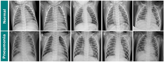
The selection of images is from routine examinations carried out in the pediatric section of the medical center. The patients, whose identities were withheld when the database was built, were aged between 1 and 5 years. The data set is composed of 6,000 images with sizes ranging from 384127 29162583. All the CXR examinations were subjected to expert analysis. The experts made a selection of good quality images and their respective diagnoses. The characteristics of this database are suitable for the validation of automatic computational methods for the classification process (Fig. 2).
Fig. 2.
Samples of each class of the CXR dataset. From left to right, sets of five images for the classes a normal, b pneumonia
Preprocessing
The pre-processing used in this approach corresponds to an adaptive equalization of the histogram. The dataset had a wide variety of CXR exams due to size and age range as well as the equipment used and the technician responsible. These conditions determine the quality of contrast and resolution of the exam, and at times poor conditions hinder the diagnosis. To work around this problem, we applied an adaptive histogram equalization based on sub-regions of the images.
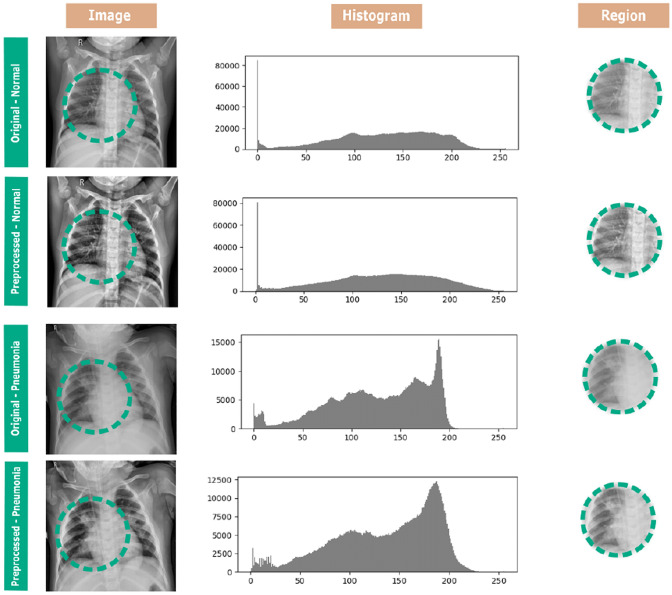
This type of equalization was used to improve the contrast throughout the exam, especially the pulmonary region. The data set sample images shown below in Fig. 3 contain areas external to the lung. If an equalization based on global imaging parameters were performed, it would be difficult to improve important lung regions for diagnosis. Figure 3 demonstrates that small regions within the lung are shown, thus highlighting a characteristic of the individual’s lung without any external influence.
Fig. 3.
Samples of each class, for classes a normal and b pneumonia, from the chest radiography data set. From left to right, we compare the original sample and the preprocessed one, with a highlight after preprocessing
The regions to be equalized individually are defined by dividing the input image into n regions of the same size. These regions are divided and equalized separately, thus providing full equalization of the image. The smaller the selected regions are, the greater the sensitization of the method is in the presence of noise. The susceptibility to unwanted information is circumvented with a contrast limit. However, if exceeded, the image pixels will be redistributed evenly to other regions before equalization. Finally, after equalizing all image regions, a bilinear interpolation is performed to remove any noise from the edges of each area.
Figure 3 shows the change due to the adaptive histogram equalization in two samples of the dataset. All the images were resized to the input size of each CNN configuration. This resizing admits low computational costs because it uses the interpolation of the nearest neighbor of the OpenCV library. The average pre-processing time for all the images of the dataset was 14.924 ± 8.710 ms.
Convolution neural networks as feature extractors
The extraction of characteristics covered in this subsection is based on the use of transfer learning from CNN. This process in a CNN can be divided into the following steps: input of the image to be processed, application of non-linear conversions that result in a set of matrices smaller than the input image [12], the formation of feature vectors [20], and implementation of this vector on a structure composed of one or more layers of multiple perceptrons, called fully connected layers [25]. One of the main consequences of using CNN, more precisely Deep Learning, consists of linking many parameters to a few samples, resulting in overfitting [34].
The main idea of transfer learning is to transfer learning from one challenge to another [17]. The use of transfer learning allows minimizing overfitting, thus maintaining the ability to generalize the approach with few samples. The pre-training carried out requires extensive and varied datasets, such as the ImageNet dataset [25]. Because of this, we selected 12 high-performance CNNs pre-trained with the ImageNet dataset. The CNNs used are in Table 2, where some important characteristics are shown (Fig. 4).
Table 2.
Configurations of convolutional neural networks used in this work
| Architectures | Highlights | Configurations | Number of features extracted |
|---|---|---|---|
| VGG [29] | Factorized Convolution, a regularization strategy to avoid overfitting | VGG16 | 512 |
| VGG19 | 512 | ||
| Inception [30] | Inception Module, a building block for reducing the amount of extracted parameters | InceptionV3 | 2048 |
| InceptionResNetV2 | 1536 | ||
| ResNet [13] | Residual Block, the building block focused on vanishing-gradient optimizing | ResNet50 | 2048 |
| NASNet [35] | NASNet search space, a new architecture model build from the dataset of interest | NASNetLarge | 4032 |
| NASNetMobile | 1056 | ||
| Xception [3] | Depthwise Separable Convolution layers, the spatial and cross-channel correlation is separated | Xception | 2048 |
| MobileNet [14] | Two news hyper-parameters in the Xception model, which are Width Multiplier, Resolution Multiplier | MobileNet | 1024 |
| MobileNetV2 | 1280 | ||
| DenseNet [15] | Dense Block, a block that covers interconnects all layers | DenseNet121 | 1024 |
| DenseNet169 | 1664 | ||
| DenseNet201 | 1920 |
Fig. 4.
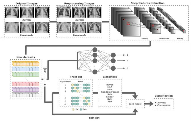
Method flow
In the pre-trained CNNs, we preserved the network parameters from the original papers and made changes in the network structures to allow transfer learning. As shown in 4, the difference in the structure consists of removing the fully connected layers, responsible for the characteristic high computational cost, and the training/classification of the network [7, 17]. In summary, the new structure’s output no longer corresponds to each class’s probabilities but rather to an extensive set of characteristic vectors. The number of features extracted from each configuration used is shown in Table 2. Thus, the set of features of each configuration consists of the generation of a new dataset.
All the CNNs used in the transfer learning process of this approach were subjected to the extraction of the same number of samples. The creation of the new dataset using deep feature extraction comes from 80% of the chest X-ray dataset, which is 4,800 images. This number of original images and the number of features extracted by each configuration, as seen in Table 2, demonstrates the large number of features produced by this method, which means that the classifiers can be trained robustly and reliably.
Classification
The classification is performed after obtaining the attributes on CNN. In this section, the five machine learning approaches that were employed in this step are described: Naive Bayes, Multilayer Perceptron (MLP), k-Nearest Neighbor (kNN), Random Forest (RF), and Support Vector Machines (SVM).
The Naive Bayes classifier consists of a group of supervised classifiers. Its machine learning approach is based on Bayes’ Decision Theory. The algorithm uses each possible class prior probability and the later probability of each possible class sample attributes. The classifier equation is based on the following aspects: conditional density, a priori probability, and probability density. This algorithm stands out for its class autonomy among the resources extracted from the sample. That is, the attributes of each possible class have resources that are not correlated with other classes.
MLP is an unsupervised algorithm designed to solve linearly non-separable problems. The structure of this neural network is composed of multiple layers. In the input layers of this network, there are the resource vectors that represent the sample. Pulses are produced in the hidden layers for sensitizing and modeling the weights between the layers interconnected with the error backpropagation algorithm. In the output layers, the value of each perceptron represents the network output for each possible sample class.
kNN is based on determining the class of an unknown sample from the spatial distribution of resources. Therefore, it is possible to identify the nearest k samples. The determination of similarity between the chosen samples is given by calculating the distance between the samples. The equation for the commonly used distance is the Euclidean distance.
RF estimates a sequence of interrelated conditionals from the training resources presented to the classifier. Conditionals are adjusted using an ensemble approach called random bagging. The main advantage of this classification method is that there is no overfitting, even with an increase in the number of trees.
SVM are classification methods based on changing the data distribution space. SVM performs the classification of an unknown sample based on the statistical learning acquired with the resources presented during the training. Statistical learning is possible from the determination of the hyperplanes that separate the data. The plotted hyperplane is defined according to the kernel used in training. There are linear, polynomial, and Radial Basis Function (RBF) kernels.
As mentioned in Sect. 3.4 for training and testing, 80% and 20% of the dataset were used, respectively. The training and test models used in the classifiers described in this section will be described in the items below. The sequence of the process and dimensioning for all classifiers were carried out equally, resulting in Table 4.
Table 4.
Accuracy, F1 score, Sensitivity, Precision, Extraction time, Training time (TrT), and Test time (TsT) obtained by classifying features extracted by different combinations of CNN architectures and features classifiers
| CNN | Classifier | Accuracy (%) | F1 score (%) | Sensitivity (%) | Precision(%) | Extraction time (ms) | Training time (s) | Test time (ms) |
|---|---|---|---|---|---|---|---|---|
| NASNetMobile | Bayes | 80.392 ± 1.471 | 81.142±1.377 | 80.392±1.471 | 83.221±1.190 | 47.332 ± 1.928 | 0.5479±0.345 | 0.050±0.034 |
| MLP | 93.259±0.328 | 93.279±0.317 | 93.259±0.328 | 93.307±0.302 | 1283.897±158.429 | 0.026±0.009 | ||
| Nearest Neighbors | 89.044±1.203 | 89.169±1.092 | 89.044±1.203 | 89.535±0.847 | 0.383±0.020 | 14.627±0.402 | ||
| RF | 87.150±2.894 | 87.599±2.602 | 87.150±2.894 | 89.496±1.298 | 153.024±4.645 | 4.862±2.414 | ||
| SVM Linear | 83.038±5.165 | 83.900±4.831 | 83.038±5.165 | 89.341±1.828 | 74.485±4.740 | 10.390±0.257 | ||
| SVM Polynomial | 63.771±18.362 | 51.538±20.011 | 63.771±18.362 | 44.039±18.362 | 64.385±5.740 | 37.749±0.293 | ||
| SVM RBF | 87.628±4.863 | 86.544±7.129 | 87.628±4.863 | 88.903±3.641 | 225.685±37.106 | 15.320±2.733 | ||
| Xception | Bayes | 87.986±0.522 | 88.345±0.495 | 87.986±0.522 | 89.477±0.440 | 108.338 ± 1.728 | 1.196±0.717 | 0.024±0.004 |
| MLP | 95.188±0.335 | 95.166±0.332 | 95.188±0.335 | 95.166±0.333 | 3592.964±259.828 | 0.204±0.111 | ||
| Nearest Neighbors | 93.618±0.954 | 93.651±0.936 | 93.618±0.954 | 93.709±0.909 | 2.7631±1.055 | 28.666±0.401 | ||
| RF | 92.321±0.833 | 92.061±0.967 | 92.321±0.833 | 92.466±0.660 | 1206.235±31.802 | 6.891±1.732 | ||
| SVM Linear | 95.666±0.379 | 95.661±0.377 | 95.666±0.379 | 95.662±0.375 | 148.377±2.667 | 14.083±0.498 | ||
| SVM Polynomial | 76.331±6.758 | 67.134±11.181 | 76.331±6.758 | 60.526±14.612 | 127.277±3.767 | 72.632±0.698 | ||
| SVM RBF | 94.983±0.932 | 94.881±0.979 | 94.983±0.932 | 95.030±0.907 | 178.985±33.990 | 26.651±0.142 | ||
| MobileNet | Bayes | 91.553±0.648 | 91.732±0.617 | 91.553±0.648 | 92.276±0.517 | 19.447 ± 0.651 | 0.5849±0.504 | 0.047±0.061 |
| MLP | 95.358±0.475 | 95.336±0.464 | 95.358±0.475 | 95.342±0.478 | 584.750±67.986 | 0.157±0.149 | ||
| Nearest Neighbors | 95.137±0.291 | 95.162±0.283 | 95.137±0.291 | 95.214±0.267 | 2.291±2.210 | 12.140±0.364 | ||
| RF | 94.317±0.533 | 94.278±0.534 | 94.317±0.533 | 94.284±0.547 | 469.650±12.416 | 6.070±2.112 | ||
| SVM Linear | 95.290±0.595 | 95.311±0.586 | 95.290±0.595 | 95.348±0.570 | 75.606±15.417 | 5.587±0.111 | ||
| SVM polynomial | 96.177±0.723 | 96.161±0.727 | 96.177±0.723 | 96.172±0.734 | 62.206±18.617 | 8.524±0.915 | ||
| SVM RBF | 95.853±0.751 | 95.844±0.726 | 95.853±0.751 | 95.866±0.694 | 139.965±12.778 | 9.206±2.161 | ||
| DenseNet121 | Bayes | 86.826±0.783 | 86.631±0.769 | 86.826±0.783 | 86.584±0.774 | 72.683 ± 0.749 | 0.526±0.661 | 0.016±0.351 |
| MLP | 95.717±0.302 | 95.717±0.311 | 95.717±0.302 | 95.722±0.320 | 2019.860±67.986 | 0.039±0.010 | ||
| Nearest neighbors | 94.198±0.378 | 94.251±0.364 | 94.198±0.378 | 94.378±0.328 | 1.996±2.720 | 14.402±0.355 | ||
| RF | 94.556±0.360 | 94.528±0.336 | 94.556±0.360 | 94.574±0.332 | 507.653±11.816 | 5.871±1.613 | ||
| SVM linear | 94.881±0.591 | 94.948±0.572 | 94.881±0.591 | 95.155±0.509 | 134.274±47.817 | 6.073±0.305 | ||
| SVM polynomial | 66.126±20.064 | 56.317±24.237 | 66.126±20.064 | 51.149±25.882 | 101.674±49.817 | 36.615±0.194 | ||
| SVM RBF | 95.768±0.220 | 95.772±0.197 | 95.768±0.220 | 95.808±0.142 | 222.004±88.078 | 9.322±2.201 | ||
| DenseNet169 | Bayes | 90.324±0.555 | 89.985±0.614 | 90.324±0.555 | 90.283±0.565 | 90.651 ± 0.830 | 0.918±0.541 | 0.019± 0.092 |
| MLP | 96.007±0.394 | 95.997±0.375 | 96.007±0.394 | 96.022±0.359 | 1797.904±109.458 | 0.169±0.078 | ||
| Nearest neighbors | 94.522±0.419 | 94.559±0.405 | 94.522±0.419 | 94.633±0.374 | 2.355±2.210 | 23.841±0.495 | ||
| RF | 94.590±0.417 | 94.550±0.407 | 94.590±0.417 | 94.580±0.420 | 1533.250±61.574 | 5.874±1.953 | ||
| SVM linear | 95.802±0.662 | 95.840±0.630 | 95.802±0.662 | 95.957±0.498 | 223.547±27.513 | 8.92±0.512 | ||
| SVM polynomial | 45.410±22.488 | 31.527±24.508 | 45.410±22.488 | 25.678±22.488 | 183.123±31.613 | 59.115±0.406 | ||
| SVM RBF | 96.212±0.444 | 96.197±0.433 | 96.212±0.444 | 96.228±0.434 | 191.653±40.839 | 14.366±2.462 | ||
| DenseNet201 | Bayes | 90.904±0.352 | 90.639±0.401 | 90.904±0.352 | 90.844±0.350 | 114.376 ± 0.898 | 3.107±1.722 | 0.021±0.092 |
| MLP | 96.331±0.683 | 96.329±0.677 | 96.331±0.683 | 96.338±0.682 | 596.263±88.912 | 0.149±0.129 | ||
| Nearest neighbors | 94.898±0.698 | 94.926±0.687 | 94.898±0.698 | 94.983±0.670 | 1.025±0.415 | 27.472±0.093 | ||
| RF | 94.949±0.453 | 94.950±0.461 | 94.949±0.453 | 94.970±0.461 | 508.184±13.306 | 4.064±2.110 | ||
| SVM linear | 95.717±0.238 | 95.768±0.238 | 95.717±0.238 | 95.943±0.268 | 138.142±33.954 | 10.613±0.759 | ||
| SVM polynomial | 63.771±18.362 | 51.538±20.011 | 63.771±18.362 | 44.039±18.362 | 108.342±38.154 | 32.620±0.362 | ||
| SVM RBF | 96.416±0.492 | 96.415±0.489 | 96.416±0.492 | 96.427±0.484 | 284.151±23.886 | 17.863±4.141 | ||
| VGG16 | Bayes | 88.840±0.837 | 88.066±0.913 | 88.840±0.837 | 89.360±0.946 | 96.921 ± 1.470 | 0.154±0.0526 | 0.015±0.01 |
| MLP | 95.444±0.284 | 95.427±0.284 | 95.444±0.284 | 95.425±0.284 | 1850.59±107.380 | 0.037±0.026 | ||
| Nearest neighbors | 94.966±0.498 | 94.926±0.495 | 94.966±0.498 | 94.933±0.502 | 0.3745±0.155 | 7.947±0.504 | ||
| RF | 94.078±0.605 | 94.070±0.593 | 94.078±0.605 | 94.073±0.588 | 939.220±35.012 | 5.864±2.330 | ||
| SVM linear | 94.863±0.799 | 94.921±0.777 | 94.863±0.799 | 95.077±0.711 | 50.683±15.664 | 3.585±0.209 | ||
| SVM polynomial | 67.491±21.467 | 57.576±25.827 | 67.491±21.467 | 51.849±26.917 | 47.132±18.164 | 17.610±1.386 | ||
| SVM RBF | 96.007±0.288 | 96.001±0.289 | 96.007±0.288 | 96.000±0.292 | 69.159±2.775 | 5.302±0.027 | ||
| VGG19 | Bayes | 88.089±0.861 | 87.246±0.978 | 88.089±0.861 | 88.513±0.938 | 121.694 ± 1.517 | 0.2276±0.075 | 0.03±0.03 |
| MLP | 95.461±0.668 | 95.455±0.648 | 95.461±0.668 | 95.471±0.624 | 1850.59±107.380 | 0.133±0.094 | ||
| Nearest neighbors | 94.608±0.907 | 94.563±0.921 | 94.608±0.907 | 94.566±0.923 | 0.288±0.148 | 8.173±0.734 | ||
| RF | 94.164±0.653 | 94.113±0.653 | 94.164±0.653 | 94.114±0.665 | 118.690±3.456 | 7.271±1.175 | ||
| SVM linear | 95.529±0.299 | 95.573±0.291 | 95.529±0.299 | 95.698±0.271 | 28.096±4.723 | 3.373±0.276 | ||
| SVM polynomial | 60.887±28.226 | 52.255±34.683 | 60.887±28.226 | 49.182±36.603 | 22.136±5.123 | 18.145±0.440 | ||
| SVM RBF | 96.468±0.644 | 96.461±0.644 | 96.468±0.644 | 96.463±0.647 | 43.972±14.761 | 5.570±2.032 | ||
| InceptionV3 | Bayes | 86.826±0.783 | 86.631±0.769 | 86.826±0.783 | 86.584±0.774 | 66.000 ± 0.908 | 0.989±0.322 | 0.039±0.029 |
| MLP | 93.925±0.549 | 93.897±0.555 | 93.925±0.549 | 93.893±0.558 | 3270.333±294.801 | 0.158±0.128 | ||
| Nearest neighbors | 92.167±0.739 | 92.171±0.743 | 92.167±0.739 | 92.190±0.744 | 2.854±2.347 | 28.876±0.498 | ||
| RF | 92.372±0.631 | 92.227±0.711 | 92.372±0.631 | 92.331±0.607 | 1805±69.116 | 5.075±2.292 | ||
| SVM linear | 93.669±0.469 | 93.734±0.463 | 93.669±0.469 | 93.880±0.454 | 188.825±36.993 | 20.035±1.538 | ||
| SVM polynomial | 54.590±22.488 | 41.533±24.508 | 54.590±22.488 | 34.858±22.488 | 110.250±39.490 | 72.814±0.460 | ||
| SVM RBF | 93.072±2.697 | 92.840±3.106 | 93.072±2.697 | 93.211±2.355 | 378.215±57.102 | 30.017±4.826 | ||
| InceptionResNetV2 | Bayes | 81.280±0.759 | 81.791±0.698 | 81.280±0.759 | 82.893±0.652 | 158.771 ± 1.248 | 1.36211±0.467 | 0.017±0.064 |
| MLP | 93.754±0.469 | 93.709±0.459 | 93.754±0.469 | 93.774±0.393 | 724.022±97.302 | 0.250±0.117 | ||
| Nearest neighbors | 88.959±1.053 | 89.282±0.969 | 88.959±1.053 | 90.360±0.629 | 1.615±1.445 | 20.464±0.019 | ||
| RF | 91.092±1.158 | 91.003±1.109 | 91.092±1.158 | 91.055±1.088 | 800.504±30.570 | 3.056±1.800 | ||
| SVM linear | 92.935±0.450 | 93.025±0.453 | 92.935±0.450 | 93.259±0.492 | 113.940±22.140 | 14.001±0.738 | ||
| SVM polynomial | 74.863±2.974 | 68.497±8.693 | 74.863±2.974 | 65.793±15.524 | 101.340±19.140 | 51.355±6.868 | ||
| SVM RBF | 93.908±0.844 | 93.868±0.854 | 93.908±0.844 | 93.883±0.871 | 128.050±18.991 | 18.942±2.977 | ||
| ResNet50 | Bayes | 86.433±1.384 | 86.768±1.269 | 86.433±1.384 | 87.614±0.936 | 57.701 ± 1.134 | 1.362±0.461 | 0.046± 0.027 |
| MLP | 94.539±0.280 | 94.531±0.286 | 94.539±0.280 | 94.538±0.297 | 724.0229±97.079 | 0.159±0.083 | ||
| Nearest neighbors | 93.618±0.671 | 93.670±0.653 | 93.618±0.671 | 93.784±0.622 | 1.616±1.447 | 28.474±0.012 | ||
| RF | 93.584±0.587 | 93.537±0.570 | 93.584±0.587 | 93.545±0.582 | 800.504±30.570 | 3.464±1.508 | ||
| SVM linear | 94.539±0.831 | 94.587±0.804 | 94.539±0.831 | 94.717±0.739 | 113.940±22.140 | 14.714±0.577 | ||
| SVM polynomial | 27.048±0.000 | 11.517±0.000 | 27.048±0.000 | 7.316±0.000 | 99.340±25.340 | 72.765±0.299 | ||
| SVM RBF | 94.983±0.513 | 94.935±0.516 | 94.983±0.513 | 94.949±0.526 | 128.052±18.853 | 25.461± 5.514 | ||
| NASNetLarge | Bayes | 82.611±1.138 | 83.107±1.032 | 82.611±1.138 | 84.261±0.774 | 313.715 ± 2.359 | 1.492±0.522 | 0.042±0.113 |
| MLP | 94.437±1.004 | 94.411±1.009 | 94.437±1.004 | 94.430±1.011 | 2486.365±282.362 | 0.215±0.102 | ||
| Nearest neighbors | 89.863±1.141 | 90.085±1.060 | 89.863±1.141 | 90.733±0.823 | 2.436±0.428 | 56.197±0.496 | ||
| RF | 91.809±1.220 | 91.722±1.190 | 91.809±1.220 | 91.815±1.110 | 862.818±27.096 | 5.496±2.070 | ||
| SVM linear | 94.488±0.585 | 94.527±0.563 | 94.488±0.585 | 94.611±0.516 | 304.663±31.350 | 36.452±0.933 | ||
| SVM polynomial | 36.229±18.362 | 21.522±20.011 | 36.229±18.362 | 16.497±18.362 | 283.125±34.120 | 143.020±0.448 | ||
| SVM RBF | 93.942±1.473 | 93.818±1.615 | 93.942±1.473 | 93.975±1.365 | 441.346±6.816 | 52.329±7.522 |
Bold values highlight the performance of the proposed algorithm
The hyperparameters used in classifier training come from a random search of 20 interactions. Table 3 contains information and definitions of the classifier parameters in the random search. The random search configures the best configuration for each classifier, which is saved regarding the average obtained in cross-validation. The tenfold cross-validation for each classifier uses 80% of the dataset. For the Naive Bayes Classifier, we did not use tenfold cross-validation.
Table 3.
Setup to search for hyperparameters of the classifiers
| Classifier | Search type | Parameter | Setup |
|---|---|---|---|
| Naive Bayes | – | – | Gaussian Probability Density Function |
| RF | Random | Number of estimators | 50–3000 in steps of 50 |
| criterion | Gini or entropy | ||
| MLP | Random | Neurons in hidden layer | 2–1000 |
| algorithm | Levenberg–Marquardt method | ||
| kNN | Grid | number of neighbors | 3, 5, 7, 9, 11, 13, 15 |
| SVM (linear kernel) | Random | C | to |
| SVM (RBF kernel) | Random | C | to |
| to |
After acquiring the best configuration for the classifiers, they were used with the remaining 20% of the data set to determine if the CXR exam belonged to an individual with pneumonia or not.
IoT framework
The Lapisco Image Interface for Development of Applications (LINDA) system consists of an IoT framework characterized by accessibility and medical diagnostics assistance. These characteristics are defined by accessing the system from any portable with an internet connection. The proposal is to insert this real-time system to detect pneumonia as part of the preliminary diagnostic process. Figure 5 shows the LINDA system’s characteristic flowchart, with each step divided and described in the image caption.
Fig. 5.
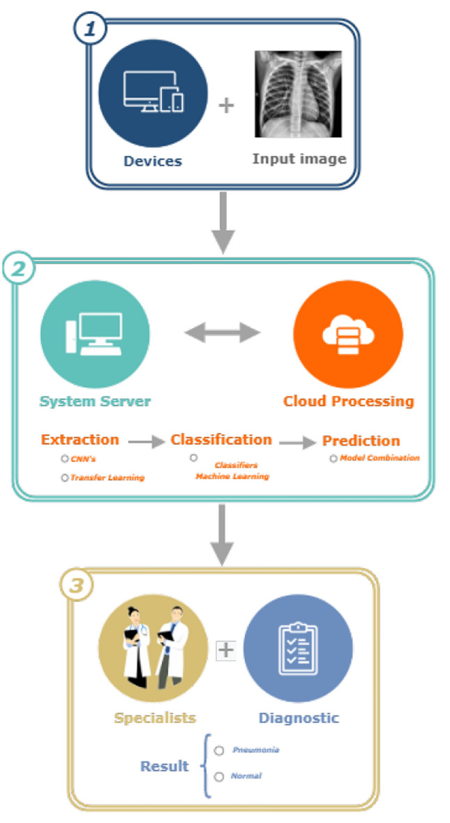
LINDA system structure
This IoT framework is structured in the communication of a web service with a cloud processing service. The web service is developed in the Java language, which allows the easy manipulation of the data and settings necessary to generate the classification results. This aspect of the platform is responsible too for communicating mobile devices and computers with the computational cloud.
Standardizing the images inserted by the user enables the platform to be compatible with different types of exams, thus demonstrating its robustness. Standardization consists of adjusting the size, format, and color conversion of the inserted images. Furthermore, the user is able to control and have a free choice of combinations, which, once produced, only need to be refilled.
The hardware and software configuration responsible for the processing was an AMD Ryzen 7 2700X Eight-Core with 16 threads and 32 Gb of memory, running Linux Ubuntu 16.04 64-bit operating system with no Graphical Processing Unit (GPU), Java version 1.8.0, Python version 3, Keras v2.3.1, Scikit-Learn library v0.21.0, and OpenCV v4.1.0.
Evaluation metrics
This work evaluated 36 combinations of CNN extractors with classic classifiers. Each combination was evaluated concerning the test time and evaluation metrics, more precisely, the Accuracy (Acc), Precision (Prec), Sensitivity (Sen), and F1 score metric. The prediction time corresponds to the average prediction time of the test samples, which were 20% of the dataset used that had 1200 images.
The behavior of the classifier was evaluated using metrics obtained in the confusion matrix. Figure 6 shows the confusion matrix with the Normal and Pneumonia classes. The normal class represents a group of healthy patients. In this matrix, true positive (TP), false positive (FP), true negative (TN), and false negative (FN) are arranged in a sectioned figure in rows and columns.
Fig. 6.
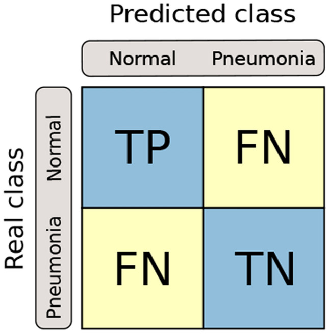
The confusion matrix structure
TP is the number of correctly classified CXR. FP is the number of times that a patient without pneumonia was classified incorrectly. TN is the number of radiographs from healthy patients that were classified correctly. FN is the number of radiographs from healthy patients that were incorrectly classified.
Equations 1–4 correspond to the respective calculations for the Accuracy (Acc), Precision, Sensitivity, and F1 score metrics. Accuracy is the frequency at which the model is correctly classifying the patient as healthy or ill. Precision checks how many patients predicted with pneumonia were actually ill. The Sensitivity (Sen) shows how many radiographs were classified as an unwanted type. F1 score is the harmonious average between Precision and Sensitivity.
| 1 |
| 2 |
| 3 |
| 4 |
Results and discussion
This section presents the computational results for the classification of radiographic images for patients with pneumonia and without pneumonia. The results achieved by this work are compared against the results obtained by other works in the literature.
Results
Tables 4 shows the mean values and their respective standard deviations for the metrics Accuracy, F1 score, Sensitivity, and Precision, in addition to the times achieved in the method’s steps. The proposed approach used twelve CNNs as extractors of image characteristics and seven classic classifiers, making up 84 combinations of pairs. The pairs of the extractor–classifier combination that reached values higher than 96.00% for the evaluative metrics Accuracy, F1 score, Sensitivity, and Precision are in bold.
A total of 19 combinations achieved 95.00% for all metrics with the test samples. The DenseNet121, VGG16, and VGG19 extractors and the MLP and SVM classifiers with the RBF kernel stood out; the MobileNet extractor reached values above 95.00% with the MLP, nearest neighbors, and the SVM classifiers with the linear, polynomial, and RBF kernels; Xception had excellent results with MLP and SVM linear; and both DenseNet169 and DenseNet201 achieved these high values with MLP, SVM linear, and SVM RBF.
The VGG19 network with the SVM-RBF achieved the highest Accuracy. This configuration gave Accuracy, F1 score, Sensitivity, and Precision averages of 96.468%, 96.461%, 96.468%, and 96.463%, respectively. In addition to this combination, six other combinations reached accuracy values above 96.00%.
Table 4 shows the extraction, training, and test times for the combinations in addition to the metrics. Knowledge of these times is essential to be aware of the computational costs. Time is also one of the crucial parameters for embedded systems. Furthermore, the standard deviation of the results here proves the stability and reliability of the proposed method.
The results show that the MLP classifier achieved the fastest test times among the combinations that reached Accuracy greater than 95.00%. This time is due to the low number of neurons in the hidden layer. The nearest neighbors had the slowest test times as it compared all the attributes extracted by the CNN.
The best combination, VGG19 with SVM-RBF, obtained the fastest training time among the combinations with Accuracy greater than 95%. The training time obtained is 43.972 ± 14.761 s, which, added to the extraction time, is less than a minute.
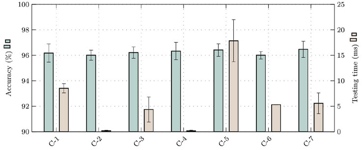
Table 5 illustrates the classes under study and the classification results obtained for the best extractor–classifier combinations obtained. More precisely, Table 5 shows the ability to differentiate between classes with the number of samples correctly and incorrectly predicted. DenseNet201 with MLP and SVM RBF obtained the lowest classification error for the reviews of patients who have not have pneumonia. In addition, MobileNet, in conjunction with SVM Polynomial and DenseNet169 with SVM RBF, achieved the smallest classification error for patients who had pneumonia. Figure 7 highlights the results obtained from the best combinations shown in Table 5, demonstrating by combination the Accuracy and the Test time per image with their respective standard deviations.
Table 5.
Confusion matrix of the extractor–classifier combinations that reached values above 96.00%
| True class | Normal | Pneumonia | ||
|---|---|---|---|---|
| Classified as | Normal | Pneumonia | Normal | Pneumonia |
| MobileNet-SVM polynomial | 291 | 26 | 18 | 837 |
| DenseNet169-MLP | 291 | 26 | 21 | 834 |
| DenseNet169-SVM RBF | 291 | 26 | 18 | 837 |
| DenseNet201-MLP | 295 | 22 | 21 | 834 |
| DenseNet201-SVM RBF | 295 | 22 | 20 | 835 |
| VGG16-SVM RBF | 292 | 25 | 22 | 833 |
| VGG19-SVM RBF | 294 | 23 | 19 | 836 |
Fig. 7.
Accuracy, and testing time for the best combinations of feature extractor with classifier. (C-1: MobileNet + SVM(Polynomial), C-2: DenseNet169 + MLP, C-3: DenseNet169 + SVM(RBF), C-4: DenseNet201 + MLP, C-5: DenseNet201 + SVM(RBF), C-6: VGG16 + SVM(RBF), and C-7: VGG19 + SVM(RBF)
Comparison with literature works
In this subsection, we compared our results with other works to evaluate and validate the proposed approach. Table 1 shows the approach, the main highlights, and disadvantages of these works. Table 6 compares the results obtained in the proposed approach with the other studies.
Table 6.
Comparison between the proposed approach with the other works in the literature
| Works | Acc (%) | F1 score (%) | Sen (%) | Prec (%) | TsT (ms) |
|---|---|---|---|---|---|
| Proposed | 96.47 | 96.46 | 96.47 | 96.46 | 5.570 |
| Ayan and Ünver [1] | 82 | 80.5 | 79.5 | 84 | 16 |
| Ayan and Ünver [1] | 87 | – | 87.5 | 87 | 20 |
| Kermany et al. [18] | 92.8 | – | 93.2 | 90.1 | – |
| Rahimzadeh et al. [27] | 91.40 | 90.52 | – | 72.83 | – |
| Chouhan et al. [4] | 96.38 | – | 99.62 | 93.28 | 161 |
Bold values highlight the performance of the proposed algorithm
The analysis of 84 different combinations demonstrated that the VGG19 extractor combined with the SVM classifier with the RBF kernel was the best model for detecting pneumonia in CXR images. This approach achieved higher values in the metrics Accuracy, F1 score, and Precision than the other works in the literature evaluated here.
Another highlight of the proposed method is the low computational cost obtained with the extractor–classifier combinations. The proposed approach obtained lower average times per image than the other approaches.
The average value of the test time obtained in the VGG19 approach with SVM-RBF reached the time of 5.570 ± 2.032 ms. Table 6 shows that our approach is three and four times faster than the work by Ayan, and Ünver [1] work with the VGG16, and Xception approaches. Also, it is 28 times faster than the work of Chouhan et al. [4].
In addition to achieving the highest values of the metrics, Accuracy, F1 score, and Precision combined with the fastest time per image, our approach is the only one that linked the proposed model to a real-time IoT system. As our work also focuses on the availability of access by specialists using a consolidated IoT system, the user can insert an image of the radiographic examination into the system, and seconds later, receives the diagnosis based on the radiography. Thus, the specialist will have the support of the system and more confidence in diagnosing a patient. The idea is not to replace the professional but to speed up and confirm the diagnosis of traditional methods. Consequently, improving the quality of treatment.
Thus, in summary, the main results of this work are
The CNN VGG19 and the SVM classifier with the RBF kernel obtained the best model for detecting pneumonia in CXR images.
The approach achieved 96.47% accuracy, 96.46% F1 score, 96.47% sensitivity, and 96.46% accuracy.
The time per image is 5.570 microseconds.
Availability of the approach in an IoT system consolidated by the medical community.
Conclusion and future works
This work proposes a method using CNNs as extractors of image characteristics and classic classifiers in a real-time IoT system to aid in the diagnosis of pneumonia in children. An extensive comparison of the method was carried out with twelve CNNs combined with seven classifiers equally tested on 1,200 CXR images of children.
The results were compared with the principal works of the literature in this area. The results of the proposed method showed that the combination of the convolutional neural network VGG19 and the classic SVM classifier with the RBF kernel was the best model. The results obtained in the metrics Accuracy, F1 score and Precision were, respectively, 96.47%, 96.46%, and 96.46%. This combination also had the lowest times compared to the other works reported in the literature, that is, 43.972 ± 14.761 s and 5.570 ± 2.032 ms for the training and classification times, respectively.
Another major contribution of this work is its availability to anyone through an IoT system consolidated in the medical community. The system enables the insertion of an X-ray exam image and produces the result in real time. LINDA sorts the image and returns a result confirming the presence or absence of pneumonia. Consequently, information from this system will help make the diagnosis more accurate and consistent.
The perspective of future work is focused on the segmentation of the regions of the lungs when and where pneumonia is present. Another perspective for future work is a historical progressive monitoring of the patient and affected region, assisting the pulmonologist in a visual analysis of the patient’s on-going condition.
Acknowledgements
The authors are grateful to the Deanship of Scientific Research at King Saud University for funding this work through Vice Deanship of Scientific Research Chairs: Research Chair of Pervasive and Mobile Computing. Mohammad Mehedi Hassan is the corresponding author of this paper.
Biographies
João Victor Souza das Chagas
is currently enrolled in the Mechatronics Engineer program at the Federal Institute of Ceará (IFCE), Brazil. He is also a member of the Laboratory of Image Processing, Signals, and Applied Computing (LAPISCO). His research area mainly focuses on the classification and segmentation of medical imaging, applying digital image processing techniques, deep learning, and artificial intelligence.
Douglas de Araújo Rodrigues
is a Mechanical Engineer and Master student in Teleinformatics Engineering from the Federal University of Ceará (UFC). Member of the Laboratory of Image Processing, Signals, and Applied Computing (LAPISCO). Extensive experience in Applied Computing and 3D Visualization and Processing, with a specific interest in Pattern Recognition, Artificial Intelligence, Machine Learning, and Image Processing and Analysis.
Roberto Fernandes Ivo
is a Mechanical Engineer and Master student in Teleinformatics Engineering from the Federal University of Ceará (UFC). Member of the Laboratory of Image Processing, Signals, and Applied Computing (LAPISCO). Extensive experience in Applied Computing and 3D Visualization and Processing, with a specific interest in Pattern Recognition, Artificial Intelligence, Machine Learning, and Image Processing and Analysis.
Mohammad Mehedi Hassan
is currently a Full Professor of Information Systems Department in the College of Computer and Information Sciences (CCIS), King Saud University (KSU), Riyadh, Kingdom of Saudi Arabia. He received his Ph.D. degree in Computer Engineering from Kyung Hee University, South Korea in February 2011. He has authored and coauthored around 180+ publications including refereed IEEE/ACM/Springer/Elsevier journals, conference papers, books, and book chapters. Recently, his 4 publications have been recognized as the ESI Highly Cited Papers. He has served as chair, and Technical Program Committee member in numerous reputed international conferences/workshops such as IEEE CCNC, ACM BodyNets, IEEE HPCC etc. He is a recipient of a number of awards including Best Journal Paper Award from IEEE Systems Journal in 2018, Best Paper Award from CloudComp in 2014 conference, and the Excellence in Research Award from King Saud University (2 times in row, 2015 & 2016). His research interests include Cloud computing, Edge computing, Internet of things, Body sensor network, Big data, Deep learning, Mobile cloud, Smart computing, Wireless sensor network, 5G network, and social network. He is a Senior Member of the IEEE.
Victor Hugo C. de Albuquerque
is a professor and senior researcher at the LAPISCO/IFCE and ARMTEC Tecnologia em Robótica, Brazil. He has a Ph.D in Mechanical Engineering from the Federal University of Paraíba (UFPB, 2010), an MSc in Teleinformatics Engineering from the Federal University of Ceará (UFC, 2007), and he graduated in Mechatronics Engineering at the Federal Center of Technological Education of Ceará (CEFETCE, 2006). He is a specialist, mainly, in IoT, Machine/Deep Learning, Pattern Recognition, Robotic.
Pedro P. Rebouças Filho
is graduated in Mechatronics Engineering from Federal Institute of Ceará, Brasil (2008). In 2010, he obtained a M.Sc. in Teleinformatics Engineering, in the field of Biomedical engineering, also at Federal University of Ceará. In 2013, he obtained a Ph.D. degree in Teleinformatics Engineering from the same University. He was Assistant Professor in the Federal Institute of Ceará since 2008. He has been evolved in several research projects in the field of Computational Vision, Medical Image and Embedded System, both as researcher and as scientific coordinator. His main research areas include Computational Vision, Scientific Visualization, Human-Computer Interaction, Embedded System, and applied Artificial Intelligence.
Footnotes
Publisher's Note
Springer Nature remains neutral with regard to jurisdictional claims in published maps and institutional affiliations.
Contributor Information
João Victor S. das Chagas, Email: victor.souza@lapisco.ifce.edu.br.
Douglas de A. Rodrigues, Email: douglas@lapisco.ifce.edu.br.
Roberto F. Ivo, Email: robertoivo@lapisco.ifce.edu.br
Mohammad Mehedi Hassan, Email: mmhassan@Ksu.edu.sa.
Victor Hugo C. de Albuquerque, Email: victor.albuquerque@ieee.org
Pedro P. Rebouças Filho, Email: pedrosarf@ifce.edu.br.
References
- 1.Ayan, E., Ünver, H.M.: Diagnosis of pneumonia from chest X-ray images using deep learning. In: 2019 Scientific Meeting on Electrical-Electronics Biomedical Engineering and Computer Science (EBBT), pp. 1–5 (2019). 10.1109/EBBT.2019.8741582
- 2.Brinker TJ, Hekler A, Utikal JS, Grabe N, Schadendorf D, Klode J, Berking C, Steeb T, Enk AH, von Kalle C. Skin cancer classification using convolutional neural networks: systematic review. J. Med. Internet Res. 2018;20(10):e11936. doi: 10.2196/11936. [DOI] [PMC free article] [PubMed] [Google Scholar]
- 3.Chollet, F.: Xception: Deep learning with depthwise separable convolutions. In: Proceedings of the IEEE conference on computer vision and pattern recognition, pp. 1251–1258 (2017). 10.1109/CVPR.2017.195
- 4.Chouhan V, Singh SK, Khamparia A, Gupta D, Tiwari P, Moreira C, Damaševičius R, de Albuquerque VHC. A novel transfer learning based approach for pneumonia detection in chest X-ray images. Appl. Sci. 2020;10:2. doi: 10.3390/app10020559. [DOI] [Google Scholar]
- 5.Daurado, C.M., et al.: Deep learning iot system for online stroke detection in skull computed tomography images. Comput. Netw. 152, 25–39 (2019). 10.1016/j.comnet.2019.01.019
- 6.de Albuquerque, V.H.C., de Rodrigues, A.D., Ivo, R.F., Peixoto, S.A., Han, T., Wu, W., Filho, P.P.R.: Fast fully automatic heart fat segmentation in computed tomography datasets. Computer. Med. Imaging Graph. 80, 101674 (2020). 10.1016/j.compmedimag.2019.101674 [DOI] [PubMed]
- 7.Dourado CM, da Silva SP, da Nóbrega RV, Barros AC, Sangaiah AK, Filho PPR, de Albuquerque VHC. A new approach for mobile robot localization based on an online IoT system. Future Gener. Comput. Syst. 2019;100:859–881. doi: 10.1016/j.future.2019.05.074. [DOI] [Google Scholar]
- 8.Farhat H, Sakr GE, Kilany R. Deep learning applications in pulmonary medical imaging: recent updates and insights on COVID-19. Mach. Vis. Appl. 2020;31(6):1–42. doi: 10.1007/s00138-020-01101-5. [DOI] [PMC free article] [PubMed] [Google Scholar]
- 9.Filho PP, Cortez P, Barros C, Albuquerque V, Tavares J. Novel and powerful 3d adaptive crisp active contour method applied in the segmentation of ct lung images. Med. Image Anal. 2017;35:503–516. doi: 10.1016/j.media.2016.09.002. [DOI] [PubMed] [Google Scholar]
- 10.Granados, J., Westerlund, T., Zheng, L., Zou, Z.: IoT platform for real-time multichannel ECG monitoring and classification with neural networks. In: Lecture Notes in Business Information Processing, pp. 181–191. Springer International Publishing (2018). 10.1007/978-3-319-94845-4\_16
- 11.Han T, Ivo RF, de Rodrigues AD, Peixoto SA, de Albuquerque VHC, Filho PPR. Cascaded volumetric fully convolutional networks for whole-heart and great vessel 3d segmentation. Future Gener. Comput. Syst. 2020;108:198–209. doi: 10.1016/j.future.2020.02.055. [DOI] [Google Scholar]
- 12.He K, Zhang X, Ren S, Sun J. Spatial pyramid pooling in deep convolutional networks for visual recognition. IEEE Trans. Pattern Anal. Mach. Intell. 2015;37(9):1904–1916. doi: 10.1109/tpami.2015.2389824. [DOI] [PubMed] [Google Scholar]
- 13.He, K., Zhang, X., Ren, S., Sun, J.: Deep residual learning for image recognition. In: Proceedings of the IEEE conference on computer vision and pattern recognition, pp. 770–778 (2016). 10.1109/CVPR.2016.90
- 14.Howard, A.G., Zhu, M., Chen, B., Kalenichenko, D., Wang, W., Weyand, T., Andreetto, M., Adam, H.: Mobilenets: Efficient convolutional neural networks for mobile vision applications. arXiv:1704.04861 (2017)
- 15.Huang, G., Liu, Z., Van Der Maaten, L., Weinberger, K.Q.: Densely connected convolutional networks. In: Proceedings of the IEEE conference on computer vision and pattern recognition, pp. 4700–4708 (2017). 10.1109/CVPR.2017.243
- 16.Jader, G., Fontineli, J., Ruiz, M., Abdalla, K., Pithon, M., Oliveira, L.: Deep instance segmentation of teeth in panoramic x-ray images. In: 2018 31st SIBGRAPI Conference on Graphics, Patterns and Images (SIBGRAPI), pp. 400–407 (2018)
- 17.Jr, C.M.D., da Silva, S.P.P., da Nóbrega, R.V.M., da S. Barros, A.C., Filho, P.P.R., de Albuquerque, V.H.C.: Deep learning IoT system for online stroke detection in skull computed tomography images. Computer Networks 152, 25–39 (2019). 10.1016/j.comnet.2019.01.019
- 18.Kermany DS, Goldbaum M, Cai W, Valentim CC, Liang H, Baxter SL, McKeown A, Yang G, Wu X, Yan F, et al. Identifying medical diagnoses and treatable diseases by image-based deep learning. Cell. 2018;172(5):1122–1131. doi: 10.1016/j.cell.2018.02.010. [DOI] [PubMed] [Google Scholar]
- 19.Kruthika KR, Maheshappa H. Cbir system using capsule networks and 3d cnn for alzheimer’s disease diagnosis. Inf. Med. Unlocked. 2019;14:59–68. doi: 10.1016/j.imu.2018.12.001. [DOI] [Google Scholar]
- 20.Lecun Y, Bottou L, Bengio Y, Haffner P. Gradient-based learning applied to document recognition. Proc. IEEE. 1998;86(11):2278–2324. doi: 10.1109/5.726791. [DOI] [Google Scholar]
- 21.Li Y, Zhang Z, Dai C, Dong Q, Badrigilan S. Accuracy of deep learning for automated detection of pneumonia using chest X-ray images: a systematic review and meta-analysis. Comput. Biol. Med. 2020;123:103898. doi: 10.1016/j.compbiomed.2020.103898. [DOI] [PubMed] [Google Scholar]
- 22.Medeiros, A.G., Guimarães, M.T., Peixoto, S.A., de O. Santos, L., da Silva Barros, A.C., de S. Rebouças, E., de Albuquerque, V.H.C., Filho, P.P.R.: A new fast morphological geodesic active contour method for lung CT image segmentation. Measurement 148, 106687 (2019). 10.1016/j.measurement.2019.05.078
- 23.Minonzio JG, Cataldo B, Olivares R, Ramiandrisoa D, Soto R, Crawford B, De Albuquerque VHC, Munoz R. Automatic classifying of patients with non-traumatic fractures based on ultrasonic guided wave spectrum image using a dynamic support vector machine. IEEE Access. 2020;8:194752–194764. doi: 10.1109/ACCESS.2020.3033480. [DOI] [Google Scholar]
- 24.Moncada-Sánchez, L.F., Salido-Ruiz, R.A., Espinoza-Valdez, A.: A medical IoT-based remote monitoring system: application on diabetic foot. In: IFMBE Proceedings, pp. 1313–1319. Springer International Publishing (2019). 10.1007/978-3-030-30648-9\_169
- 25.da Nóbrega, R.V.M., Filho, P.P.R., Rodrigues, M.B., da Silva, S.P.P., Júnior, C.M.J.M.D., de Albuquerque, V.H.C.: Lung nodule malignancy classification in chest computed tomography images using transfer learning and convolutional neural networks. Neural Comput. Appl. (2018). 10.1007/s00521-018-3895-1
- 26.Olivares R, Muñoz R, Soto R, Crawford B, Cárdenas D, Ponce A, Taramasco C. An optimized brain-based algorithm for classifying Parkinson’s disease. Appl. Sci. 2020;10:1827. doi: 10.3390/app10051827. [DOI] [Google Scholar]
- 27.Rahimzadeh M, Attar A. A modified deep convolutional neural network for detecting COVID-19 and pneumonia from chest X-ray images based on the concatenation of xception and ResNet50v2. Inf. Med. Unlocked. 2020;19:100360. doi: 10.1016/j.imu.2020.100360. [DOI] [PMC free article] [PubMed] [Google Scholar]
- 28.Sarmento RM, Vasconcelos FF, Filho PPR, de Albuquerque VHC. An iot platform for the analysis of brain ct images based on parzen analysis. Future Gener. Comput. Syst. 2020;105:135–147. doi: 10.1016/j.future.2019.11.033. [DOI] [Google Scholar]
- 29.Simonyan, K., Zisserman, A.: Very deep convolutional networks for large-scale image recognition. arXiv:1409.1556 (2014)
- 30.Szegedy, C., Liu, W., Jia, Y., Sermanet, P., Reed, S., Anguelov, D., Erhan, D., Vanhoucke, V., Rabinovich, A.: Going deeper with convolutions. In: Proceedings of the IEEE conference on computer vision and pattern recognition, pp. 1–9 (2015)
- 31.Vasilakakis, M., Iosifidou, V., Fragkaki, P., Iakovidis, D.: Bone fracture identification in x-ray images using fuzzy wavelet features. In: 2019 IEEE 19th International Conference on Bioinformatics and Bioengineering (BIBE), pp. 726–730 (2019)
- 32.Wei R, Zhou F, Liu B, Bai X, Fu D, Li Y, Liang B, Wu Q. Convolutional neural network (cnn) based three dimensional tumor localization using single x-ray projection. IEEE Access. 2019;7:37026–37038. doi: 10.1109/ACCESS.2019.2899385. [DOI] [Google Scholar]
- 33.Yang, A.Y., Cheng, L., Shimaponda-Nawa, M., Zhu, H.: Long-bone fracture detection using artificial neural networks based on line features of X-ray images. In: 2019 IEEE symposium series on computational intelligence (SSCI), pp. 2595–2602 (2019)
- 34.Zhao, W.: Research on the deep learning of the small sample data based on transfer learning. In: AIP Conference Proceedings, p. 020018. AIP Publishing LLC (2017). 10.1063/1.4992835
- 35.Zoph, B., Le, Q.V.: Neural architecture search with reinforcement learning. arXiv:1611.01578 (2016)


