Discrimination between Metastasis and Glioblastoma Multiforme Based on Morphometric Analysis of MR Images

Abstract

BACKGROUND AND PURPOSE:

Solitary MET and GBM are difficult to distinguish by using MR imaging. Differentiation is useful before any metastatic work-up or biopsy. Our hypothesis was that MET and GBM tumors differ in morphology. Shape analysis was proposed as an indicator for discriminating these 2 types of brain pathologies. The purpose of this study was to evaluate the accuracy of this approach in the discrimination of GBMs and brain METs.

MATERIALS AND METHODS:

The dataset consisted of 33 brain MR imaging sets of untreated patients, of which 18 patients were diagnosed as having a GBM and 15 patients, as having solitary metastatic brain tumor. The MR imaging was segmented by using the K-means algorithm. The resulting set of classes (also called “clusters”) represented the variety of tissues observed. A morphology-based approach allowed discrimination of the 2 types of tumors. This approach was validated by a leave-1-patient-out procedure.

RESULTS:

A method was developed for the discrimination of GBMs and solitary METs. Two masses out of 33 were wrongly classified; the overall results were accurate in 93.9% of the observed cases.

CONCLUSIONS:

A semiautomated method based on a morphologic analysis was developed. Its application was found to be useful in the discrimination of GBM from solitary MET.

Gliomas are the most common and potentially most aggressive type of primary brain tumors in adults. GBM is the most malignant form of glioma. Its specific growth pattern is characterized by an extensive and diffuse infiltration of tumor cells in the neuropil (ie, the attenuated network of interwoven neuronal and glial cell processes). This aspect is a major factor in therapeutic surgical failure.¹ The growth of brain metastases is a complex multistage process, mediated by molecular mechanisms. The cancer cells must transform, grow, and be transported to the CNS, where they can lie dormant before invading and growing further.² The clinical symptoms associated with GBM are similar to those of brain MET. However, each tumor type has a different biologic nature and, therefore, requires different treatment strategies.^3,4 In most cases, a definitive diagnosis is based on the histopathologic analysis of a biopsy sample. However, for some cases, the differentiation of MET and GBM can be made with conventional MR imaging. For example, a solitary mass spanning the corpus callosum and both frontal lobes cannot be an MET. In other cases, it is not possible to differentiate these 2 types of tumors because the radiologic visualization of the invasive front of diffuse glioblastomas is too difficult. Generally, GBM is a solitary tumor and MET is not, but there are exceptions to this rule. In such cases, it is difficult to distinguish GBM and MET on the basis of MR imaging. The use of noninvasive methods is preferable or sometimes mandatory when a biopsy is impossible. This is the case when the mass is located near an eloquent area or when the patient's advanced age makes the procedure too dangerous. A better differentiation of the 2 types of tumor by noninvasive methods would, therefore, be beneficial.

The aggressive proliferation and invasiveness of GBM can influence the tumor morphology. Indeed, recent studies⁵ have shown that clusters of cells may separate from the tumor surface when the proliferation is high (ie, for GBM). Moreover, the tumor growth is known to be dependent on fluctuations in oxygen and nutrient supply.⁶ As a consequence, some growth directions would be favored (at a macroscopic scale) and influence the tumor morphology. Furthermore, GBMs are expected to follow a growth pattern via white matter tracts, the CSF, or meninges.⁴ Therefore, the global shape of a GBM tumor is expected to be quite complex.⁶ In contrast, METs expand more homogeneously and are anticipated to be morphologically similar to a sphere.⁷ Our hypothesis was that the morphology of the tumor could be used to efficiently differentiate solitary MET and GBM.

Various approaches have been proposed in the past years to improve the differential diagnosis of GBM and MET based on MR imaging.⁸ Most require the acquisition of data in addition to conventional MR imaging by using different techniques such as diffusion imaging,^9,10 perfusion imaging,¹¹ or MRSI,^11–13 followed by various statistical analyses.^14–19 These different works will be discussed later, but in brief, the level of inhomogeneity of a tumor was expected to be related to its nature. High-accuracy values were obtained in the distinction of glioma versus meningioma and of primary tumors (all types taken together) versus secondary tumors. However, the distinction of GBM and MET appears to be difficult, with reported correct classifications below 60%.^15,18

In this work, we focused on a semiautomated method permitting the localization and definition of the region of interest within volumetric MR imaging data. The resulting segmentation allowed defining a tumor shape that is classified as MET or GBM according to a geometric descriptor. The objective was to accurately differentiate solitary MET and GBM by using a semiautomated method for the analysis of MR imaging data.

Materials and Methods

Patients

In agreement with the local ethics committee, 33 patients with histopathologically proved GBM (18 patients) or solitary MET (15 patients) signed an informed consent to be included in the studies, part of the European Project eTUMOR. The analysis proposed here is retrospective. The patients were not subjected to any treatments before the radiologic examinations and had no prior history of surgery, chemotherapy, or radiation therapy to the intracranial structures. The group of patients included 24 men and 9 women with an age at the time of radiologic examinations in the range of 29–78 years (mean, 54.4 ± 12.5 years). This cohort consisted of regular patients of the Radboud Medical Center who were in observation between March 2006 and January 2008. Each patient's tumor type was determined by means of central consensus histopathologic validation after biopsy or after a surgical specimen had been obtained on the basis of the neuronavigation MR imaging scan.

Data Acquisition

The MR imaging data of each patient were acquired on a 3T whole-body system (Magnetom Trio; Siemens, Erlangen, Germany), following a standard protocol. The body coil was used for excitation, and a 12-channel receive-only head coil was used for reception of the MR imaging signal intensity. The MR imaging protocol included T2-weighted axial images and T1-weighted images with and without gadolinium contrast enhancement. In some cases, T1-weighted images without gadolinium were not acquired. Depending on the patient, 26 or 159 T2-weighted turbo spin-echo images (TR = 4040 ms, TE = 102 ms) were obtained with a resolution of 0.6 × 0.6 mm and a section thickness of 5 mm (leading to 26 images) or 1 mm (providing 159 T2 images). The intersection gap was set to 10% of section thickness. For T1-weighted images a 3D rapid gradient-echo sequence was used (resolution, 1 × 1 × 1 mm; TR, 2300 ms; TI, 1100 ms; TE, 4.7 ms). T1-weighted images with contrast enhancement were obtained with the same sequence after injection of 15 mL of 0.5 mol/L gadoterate meglumine (Dotarem; Guerbet, Aulnay-sous-Bois, France). The patients whose tumor could only be visualized in fewer than 5 consecutive sections were excluded from the study.

Data Analysis

The images were aligned and resampled by using Slicer, Version 2.6 (www.slicer.org) to fit to the resolution of T2-weighted images. The next part of the data analysis, toward image segmentation, is summarized in Fig 1. The aligned images were merged in a multidimensional array. The first 3 dimensions corresponded to the 3 spatial coordinates and the fourth, to the type of image (T1-weighted, T2-weighted, or gadolinium-enhanced T1). The analysis then was focused on a given section in the axial plane of the brain where the tumor lesion can be seen. The skull was removed from the image by using an in-house written program. In the following sections, we first define the variable space in which the data will be segmented. Subsequently, the procedure for selecting the region of interest is discussed in detail. Finally, in the last section the K-means algorithm used for segmentation and the morphologic analysis are presented. All the analyses described here were performed blinded to the histologic diagnosis.

Fig 1.

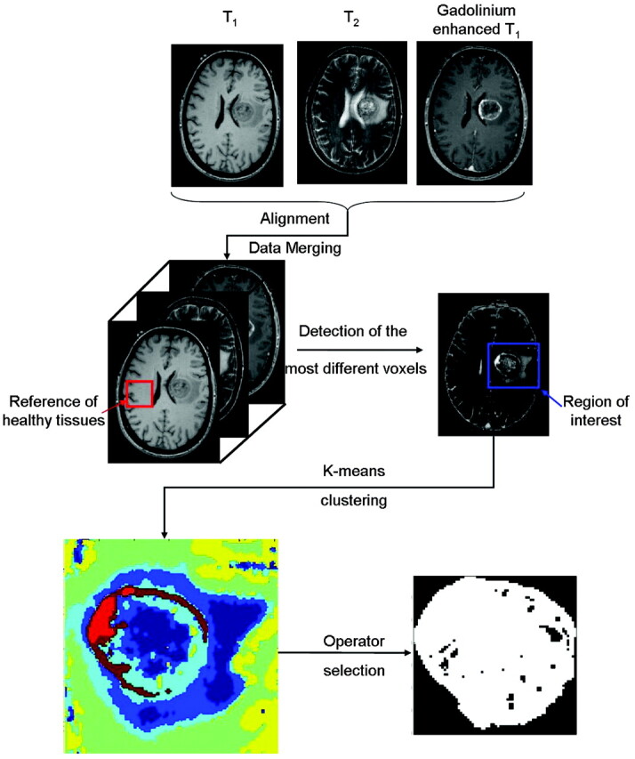
Scheme followed to select the region of interest containing the tumor and the corresponding segmented image. The area of the tumor relative to the tangent square is equal to 0.68.

Variables Space

Each voxel was considered as an independent sample. The intensities measured with precontrast T1, T2, and gadolinium-enhanced T1 MR imaging were the 3 variables that defined each voxel. The MR imaging data could be projected in a variables space in which each voxel was represented by a point at the coordinates corresponding to the intensities of each variable. Only 3 variables were used; it was then possible to represent this new space. Figure 2 gives an example of such variable space in which 100 samples are visible and regrouped in 3 classes identified as 3 clouds of points. This simulated example shows how the projection in the variable space allows regrouping the samples in different groups or “classes.”

Fig 2.

3D simulated variable space in which each point represents a voxel. Three classes of points (circle, cross, and triangle) are visible and are clearly separated from each other in this space.

Selection of the Region of Interest

The tumor was visually located by the human operator in each 2D axial plane. A region corresponding to apparently normal tissues was selected as a reference. This reference is situated in the contraparietal region, if possible at a position similar to that of the tumor. The reference region should only contain tissues expected to be normal. If the tumor was close to the interhemispheric fissure, the reference was chosen in a more distant region of the brain. The different values of voxels in the reference region were averaged to obtain single reference intensities for the 3 variables (T1, T2, and gadolinium-enhanced T1), which can be projected in the variable space as a single point. This point was then used to determine which voxels differed the most from normal tissue. This was done by calculating the Euclidian distance d_i of each voxel i to the reference r (in the variable space) as follows:

where x_i,j is the value of variable j of voxel i and x_r,j is the value of the same variable for the reference. By plotting these distances in the original MR imaging plane, we obtained a distance map. This map clearly showed a region with higher intensity corresponding to the voxels that differ most from the reference (ie, the tissues the most different from normal tissues). The region of interest (ie, the complete area affected by the tumor) could now be selected. We chose to include the entire suspected region, including additional healthy tissues in the surroundings. This selection step ensured that the entire lesion was selected and that no secondary lesion was left out. The region of interest was then segmented by using a K-means algorithm.

Segmentation Using K-Means Algorithm

The segmentation of the region of interest in tumorous and nontumorous regions requires assigning the corresponding voxels to a given number of groups. Many algorithms are available for such a task.²⁰ We chose to focus on the partitional method named K-means.²¹ This method is computationally efficient and can be applied to datasets including a high number of samples such as the MR imaging data used here.

The number of expected classes was defined beforehand. The distance (in the variable space) between each voxel and each class center (also called centroid) was computed, and every voxel was assigned to the class with the closest center. However, the position of a class center cannot be known in advance. The algorithm can be decomposed in the following points:

1. Select random “class centers.”

2. Calculate the distances between the centers and the voxels.

3. Assign all the voxels to the different classes.

4. Calculate the new class centers.

5. Return to step 2 until the convergence is achieved (the voxel assignment is the same as that in the previous iteration).

The class assignment was then color-coded, and the region of interest was depicted as presented in Fig 1.

For each image, this procedure was repeated by using different numbers of classes to optimize the description of the tumor. In general, 3–6 classes permitted the efficient distinction of healthy tissues, CSF (if present in the region of interest), edema, and tumor tissues. One type of tissue was not necessarily represented by only 1 class. A filtering algorithm was then applied to eliminate all spatial areas formed by only 1 voxel. These voxels were reattributed to other classes in accordance with the neighboring voxels. The resulting classes representing normal tissues (similar to the reference chosen) were discarded. In Fig 1, they are represented by green and yellow classes. Then the operator selected the classes corresponding to the tumor core. It is possible that the classes that outline the tumor core were also present outside the tumor core. In such a case, the 2 types of tissues (tumor core and not tumor core) were spatially easily distinguishable. Selecting 1 voxel from each area within the tumor core allows assigning all the voxels of these areas as tumor core. A binary image of the tumor was created subsequently.

Morphologic Analysis

Once the tumor shape has been defined, it is necessary to discriminate between MET and GBM. The shape of the tumor was evaluated by using a basic criterion. The largest dimension of the binary map was evaluated. This dimension was used to construct a square in which the binary tumor image fits. The ratio of white voxels in the binary map (evaluated as tumor) against the total number of pixels in that square was calculated. When the tumor core is spherical (or close to it), the binary image obtained should be a circle covering 78.5% of the square. This value comes from the area of a circle with a radius r (ie, π.r²) divided by the area of the corresponding square (ie, [2.r]²), so it is exactly π/4. Conversely when the tumor is nonspheric, the described shape does not fit the square so well, leading to a lower ratio. In most cases, the tumor lesion was visible in multiple axial sections of the volumetric MR imaging data. The ratio was calculated for each section. Means and SDs of the ratios were calculated for each patient. The mean was used as the global result for the patient.

The number of MR imaging sections analyzed per patient varied between 1 and 20 because of the size of the tumor and the spatial resolution used. The images corresponding to the lowest and highest position of the tumor lesion were discarded. In these sections, the tumor lesion is, in general, small and would probably appear circular.

The validation method used for the determination of the discriminating value, between GBM and MET, was leave-1-patient-out.²⁰ The principle was to exclude 1 patient from the dataset and then establish the discriminating value on the remaining data. The diagnosis of the patient left out was then predicted on the basis of the obtained discriminating value. This procedure was repeated for each patient, and the number of correct predictions was evaluated. In this work, 33 models can be constructed, each excluding 1 patient.

All the calculations concerning the data analysis were performed by using Matlab, Version 7.6 (MathWorks, Natick, Massachusetts).

Results

The strategy proposed here and detailed in the “Materials and Methods” section aims to distinguish GBM and MET on the basis of a simple shape descriptor. Because 3D data were available, the circularity of the tumor was evaluated in the different axial sections of the MR imaging volumes. The use of the K-means algorithm was helpful to divide the region of interest, by using the different MR images, into shapes from which the tumor core can be outlined. On-line Table 1 presents the results obtained for the 33 cases. The age, sex, histopathologic diagnosis, and type of biopsy undergone for each patient are also provided. On the basis of our method, 31 of 33 diagnoses are in correspondence with the histopathologic diagnoses. The 2 misclassified cases (cases 1 and 16) are noted. These 2 cases will be discussed later.

Metastasis Example

As an example of our approach, we describe a patient with MET (Fig 1). The tumor core is mainly described by 5 classes. Two classes (brown and orange) appeared to be limited to the gadolinium-enhanced region only (forming a border). Three classes were present within this border (probably necrosis), as well as outside, but the different areas belonging to the same class (within and outside of the tumor core) were spatially separated. Using our method, the border and the area inside this border were assigned to the tumor core. The other areas (ie, outside the tumor core) were then automatically assigned to a second class (not tumor core). The results are presented in a binary map (Fig 1, bottom right). The shape descriptor value in this section was equal to 0.68.

GBM Example

The same procedure was applied to analyze the GBM tumors. Figure 3 summarizes the main steps of the method and presents the results obtained for a representative example of GBM. The region-of-interest segmentation easily permitted isolating the tumor in brown (corresponding to the gadolinium-enhanced part of the tissues) and partly in orange and dark blue. The 2 latter classes were, however, also seen in the surrounding region. It was then necessary to select the tumoral regions. The other classes represent the healthy tissues (light blue and yellow). One can observe that the tumor shape differs from a circle, in accordance with our hypothesis. This tumor was described by our shape descriptor by a value of 0.40.

Fig 3.

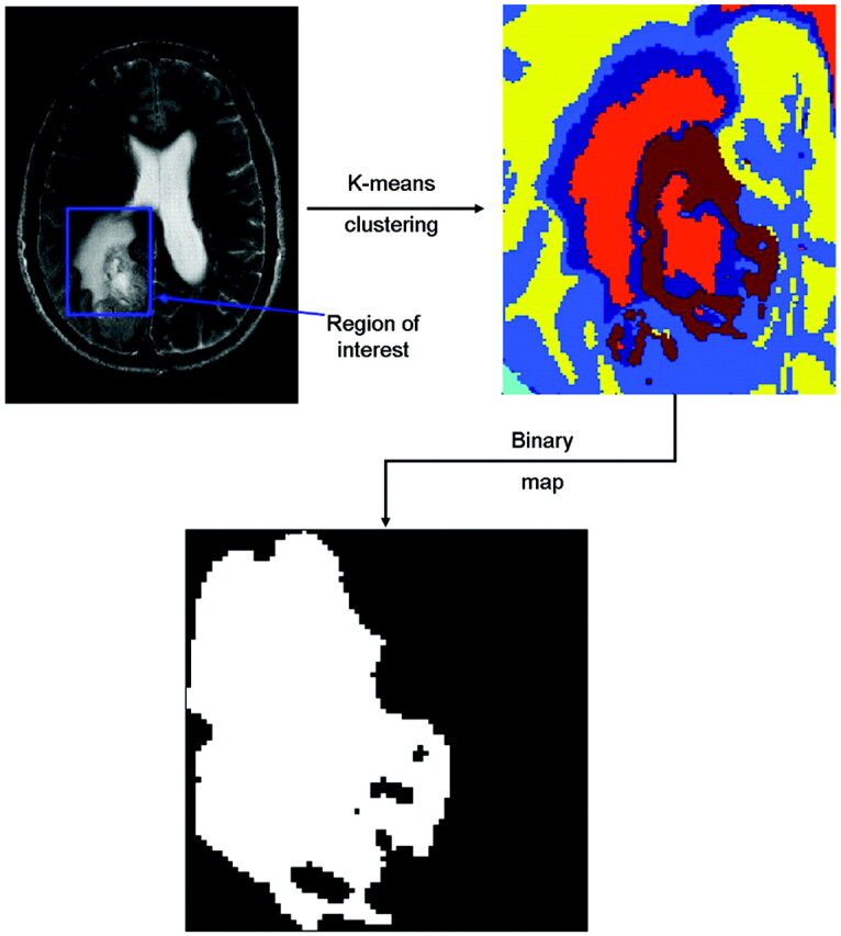
Binary representation of a GBM obtained after merging the relevant classes obtained through K-means. The relative surface of the tumor compared with the tangent square is equal to 0.40.

Global Classification and Setting of the Discriminating Value

Our approach was applied to 33 patients. Each tumor was represented by several MR imaging sections. The shape descriptor values were then used to determine the type of tumor, as can be seen in Fig 4. Each patient is represented by a vertical line, the 3 points represent the mean (center point) and the mean ± SD, the triangles correspond to patients with GBM, and the circles, to patients with MET. The 2 types of tumors form 2 distinct groups in this figure. The leave-1-patient-out cross-validation was used to set the optimal discriminating value at 0.53. Depending on which patient was excluded, the value varied between 0.51 and 0.54. The discriminating value led to the correct diagnostic prediction in 31 of 33 cases (93.9%).

Fig 4.

Mean and SD of the shape descriptors obtained on 33 patients affected by an MET (circles) or a GBM (triangles) tumor. The score obtained corresponds to the relative area of the tumor to the tangent square.

Two tumors were misclassified, 1 MET and 1 GBM. They are both represented in Fig 5. The final diagnosis for 1 of these cases was a tumor originating from an inverted papilloma. It should, therefore, have been classified as MET and not as GBM. The growth of such a tumor is known to be inhomogeneous. Therefore, the tumor was not similar to a circle and did not fulfill our primary hypothesis about the shape of MET. This case would have been identified by classic inspection of the data. The second misclassification was a GBM presenting a shape very similar to that of a sphere, which induced the classification error.

Fig 5.

Gadolinium-enhanced T1 images of an MET (A) and a GBM (B), which were misassigned by this method. The MET is noncircular; this tumor started extracranialy (at the level of the ear) and grew intracranialy. The GBM appears to be circular and is, therefore, predicted as an MET.

Discussion

As stated before, GBM and MET have different biologic natures and require different treatment strategies.^3,4 However, both types of tumors share the same clinical symptoms. Moreover, solitary MET and GBM are difficult to distinguish by using MR imaging. In most cases, a definitive diagnosis is based on a histopathologic analysis of a biopsy sample. It is, however, useful to perform this discrimination before any metastatic work-up or biopsy. The analysis of MRSI has been proved efficient to classify various types of brain tumors but not to differentiate a solitary MET from GBM.¹⁶ For the MET-versus-GBM discrimination, the MRSI analysis proposed by Devos et al¹⁵ led to a correct result in only 59% of the 126 studied spectra. A multicenter study showed that the discrimination of GBM versus MET is the most difficult one.¹⁶ Moreover, MRSI is not a readily available tool in most radiology departments and requires more examination time and expertise for proper signal-intensity processing and spectra interpretation. For that reason, pattern-recognition systems based on routinely acquired MR images have also been investigated.

Textural analysis has been proposed¹⁷ jointly with neural networks¹⁸ or support vector machines¹⁹ for classifying brain tumors. However, Georgiadis et al¹⁸ obtained a percentage of correct classification equal to 56% (on 48 cases) on the GBM/MET problem. The use of perfusion and diffusion MR imaging provided encouraging results based on the calculation of the relative cerebral blood volume,^8,22,23 but no accuracy values were provided on the discrimination of GBM from MET. Therefore, the purpose of our work was to propose a semiautomated method facilitating the differentiation of GBM from solitary metastases based on standard MR imaging data only. The method proposed here uses a semiautomated segmentation of the MR imaging data and a shape description of the tumor. It correctly diagnosed 31 of 33 patients (ie, 93.9%). The invasive growth pattern of GBM seems to influence the tumor shape enough to permit a classification on the basis of a shape descriptor.

Values Obtained in Practice

In the first example presented in the “Results” section, the value for the descriptor is 0.68. This is lower than the theoretic value of 0.78 expected for a perfectly spheric lesion. This observation is true for all the metastases cases. Two reasons may explain this deviation from the ideal case. First, the tumor description is not perfect. Some voxels are missing inside the tumor. These have been attributed to a class not used to describe the tumor core. These voxels belong to the same class as normal tissue, but this association does not necessarily mean that the voxels are healthy. Second, the tumor is not a perfect sphere but corresponds more to an ellipsoid. These 2 aspects will be addressed in future works, but they did not significantly affect the obtained results.

Limitations

The main limitation of this approach is its dependence on a human analysis of the K-means results. Indeed, an operator must select the classes representing the tumor core.

The images used during the analysis must contain complete cross-sections of the tumor. However, it is preferable to avoid considering the first and last section of the tumor volume. These 2 positions will certainly be described as circular, even if the tumor as a whole is not spheric. The size of the tumor must also be considered. The shape of a small tumor is probably still independent of the growth pattern (ie, still spheric).

The analysis proposed here relies on the segmentation of 2D axial images. The size of the tumor lesion and the resolution used during the measurement clearly influence the number of usable sections per patient. Obviously, a large number of sections gives more confidence on the diagnosis, but individual sections seem to give an acceptable estimation of the overall score. Indeed, the SD of the scores of the different sections from the different patients is relatively small. Even though for several patients 26 images were available, and for other patients 159 images, the segmentation process is performed on 1 section at the time. The number of sections is, therefore, not an issue. However, it would become a problem if the segmentation had been calculated on the complete volume at once. The resolution along the vertical axis would then vary and make the comparison between patients difficult.

Although MET and GBM are the most common tumors in the human brain, in clinical practice other brain tumor types should be considered. This method has not yet been tested with such a diverse range of tumor types. In such cases, the use of MRSI is an interesting solution because it allows distinguishing most of the tumor types from GBM and MET. Therefore, if MRSI permits concluding that the tumor is not GBM or MET, it is not necessary to apply the shape-description method proposed here.¹⁶

Thirty-three selected patients cannot be considered statistically representative of the total population affected by these 2 types of brain tumors. We plan to expand this study to new patients in the future, but the work presented here provides a proof of principle for the current method.

Future works on this specific problem will focus on the extension of this method to 3D measurements and to spectral imaging. Indeed, the method proposed here uses 1 axial plane at a time. Using the complete volume at once would probably enhance the description of the tumor shape. A study of different shape descriptors is also envisioned to detect multiple types of shapes.

Finally, this method offers an interesting complement to the classic MR imaging features. Indeed the faulty case linked to an inverting papilloma presented in Fig 5 would have obviously been detected as an abnormal case by an expert. On the other hand, the method presented here allows discriminating cases in which the usual MR imaging examination does not provide a clear answer. The segmentation of the image and shape description of the tumor are, therefore, proposed as support for a decision, but not as a replacement of the expert analysis.

Conclusions

The presented method is proposed as support for clinical diagnosis and as a first step toward a new way to differentiate brain tumors. It was found to efficiently classify solitary MET and GBM in 31 of 33 patients (93.9% of the cases). The method is proposed as a decision support tool and is not intended to replace expert assessment in diagnosis.

Abbreviations

CNS

central nervous system

GBM

glioblastoma multiforme

MET

metastasis

MRSI

MR spectroscopic imaging

References

- 1. Mangiola A, De Bonis P, Maira G, et al. Invasive tumor cells and prognosis in a selected population of patients with glioblastoma multiforme. Cancer 2008;113:841–46 [DOI] [PubMed] [Google Scholar]
- 2. Gavrilovic IT, Posner JB. Brain metastases: epidemiology and pathophysiology. J Neurooncol 2005;75:5–14 [DOI] [PubMed] [Google Scholar]
- 3. Giese A, Bjerkvig R, Berens ME, et al. Cost of migration: invasion of malignant gliomas and implications for treatment. J Clin Oncol 2003;21:1624–36 [DOI] [PubMed] [Google Scholar]
- 4. Claes A, Idema AJ, Wesseling P. Diffuse glioma growth: a guerilla war. Acta Neuropathol 2007;114:443–58. Epub 2007 Sep 6 [DOI] [PMC free article] [PubMed] [Google Scholar]
- 5. Frieboes HB, Zheng X, Sun C-H, et al. An integrated computational/experimental model of tumor invasion. Cancer Res 2006;66:1597–604 [DOI] [PubMed] [Google Scholar]
- 6. Frieboes HB, Lowengrub JS, Wise S, et al. Computer simulation of glioma growth and morphology. Neuroimage 2007;37:S59–70 [DOI] [PMC free article] [PubMed] [Google Scholar]
- 7. Stein AM, Demuth T, Mobley D, et al. A mathematical model of glioblastoma tumor spheroid invasion in a three-dimensional in vitro experiment. Biophys J 2007;92:356–65. Epub 2006 Oct 13 [DOI] [PMC free article] [PubMed] [Google Scholar]
- 8. Al-Okaili RN, Krejza J, Woo JH, et al. Intraaxial brain masses: MR imaging based diagnostic strategy—initial experience. Radiology 2007;243:539–50 [DOI] [PubMed] [Google Scholar]
- 9. Wang S, Kim S, Chawla S, et al. Differentiation between glioblastomas and solitary brain metastases using diffusion tensor imaging. Neuroimage 2009;44:653–60 [DOI] [PMC free article] [PubMed] [Google Scholar]
- 10. Chiang IC, Kuo Y-T, Lu C-Y, et al. Distinction between high-grade gliomas and solitary metastases using peritumoral 3-T magnetic resonance spectroscopy, diffusion, and perfusion imagings. Neuroradiology 2004;46:619–27. Epub 2004 Jul 9 [DOI] [PubMed] [Google Scholar]
- 11. Law M, Cha S, Knopp EA, et al. High-grade gliomas and solitary metastases: differentiation by using perfusion and proton spectroscopic MR imaging. Radiology 2002;222:715–22 [DOI] [PubMed] [Google Scholar]
- 12. Opstad KS, Murphy MM, Wilkins PR, et al. Differentiation of metastases from high-grade gliomas using short echo time 1H spectroscopy. J Magn Reson Imaging 2004;20:187–92 [DOI] [PubMed] [Google Scholar]
- 13. Fan G, Sun B, Wu Z, et al. In vivo single-voxel proton MR spectroscopy in the differentiation of high-grade gliomas and solitary metastases. Clin Radiol 2004;59:77–85 [DOI] [PubMed] [Google Scholar]
- 14. Devos A, Simonetti AW, Van Der Graaf M, et al. The use of multivariate MR imaging intensities versus metabolic data from MR spectroscopic imaging for brain tumor classification. J Magn Reson 2005;173:218–28 [DOI] [PubMed] [Google Scholar]
- 15. Devos A, Lukas L, Suykens JAK, et al. Classification of brain tumors using short echo time 1H MR spectra. J Magn Reson 2004;170:164–75 [DOI] [PubMed] [Google Scholar]
- 16. García-Gómez JM, Luts J, Julià-Sapé M, et al. Multiproject-multicenter evaluation of automatic brain tumor classification by magnetic resonance spectroscopy. Magn Resn Mater Phy 2009;22:5–18 [DOI] [PMC free article] [PubMed] [Google Scholar]
- 17. Herlidou-Même S, Constans JM, Carsin B, et al. MRI texture analysis on texture test objects, normal brain and intracranial tumors. Magn Res Imaging 2003;21:989–93 [DOI] [PubMed] [Google Scholar]
- 18. Georgiadis P, Cavouras D, Kalatzis I, et al. Improving brain tumor characterization on MRI by probabilistic neural networks and non-linear transformation of textural feature. Comput Methods Programs Biomed 2008;89:24–32. Epub 2007 Nov 28 [DOI] [PubMed] [Google Scholar]
- 19. Georgiadis P, Cavouras D, Kalatzis I, et al. Enhancing the discrimination accuracy between metastases, gliomas and meningiomas on brain MRI by volumetric textural features and ensemble pattern recognition methods. Magn Res Imaging 2009;27:120–30 [DOI] [PubMed] [Google Scholar]
- 20. Massart DL, Vandeginste BG, Buydens LMC, et al. Handbook of Chemometrics and Qualimetrics: Part B. Amsterdam, the Netherlands: Elsevier; 1998 [Google Scholar]
- 21. McQueen J. Some methods for classification and analysis of multivariate observations. In: Le Cam L, Neyman J. eds. Proceedings of the Fifth Berkeley Symposium on Mathematical Statistics and Probability. Berkeley, California: University of California; 1967:281–97 [Google Scholar]
- 22. Calli C, Kitis O, Yunten N, et al. Perfusion and diffusion MR imaging in enhancing malignant cerebral tumors. Eur Radiol 2006;58:394–403 [DOI] [PubMed] [Google Scholar]
- 23. Rollin N, Guyotat J, Streichenberger N, et al. Clinical relevance of diffusion and perfusion magnetic resonance imaging in assessing intra-axial brain tumors. Neuroradiology 2006;48:150–59 [DOI] [PubMed] [Google Scholar]
Associated Data
This section collects any data citations, data availability statements, or supplementary materials included in this article.