A Unified Scatter Rejection and Correction Method for Cone Beam Computed Tomography

Abstract

Purpose:

Scattered radiation is the primary cause of image quality degradation in flat panel detector-based cone beam CT (CBCT). While recently introduced 2D antiscatter grids reject the majority of scatter fluence, the small percentage of scatter fluence still transmitted to the detector remains a major challenge for implementation of quantitative imaging techniques such as dual energy imaging in CBCT. Additionally, this residual scatter is also a major source of grid-induced artifacts, which impedes implementation of 2D grids in CBCT.

We therefore present a new method to achieve both robust scatter rejection and residual scatter correction using a 2D antiscatter grid; in doing so, we expand the role of 2D grids from mere scatter rejection devices to scatter measurement devices.

Method:

In our method, the radiopaque septa of the 2D grid emulate a micro array of beam-stops placed on the detector which introduce spatially periodic septal shadows. By selecting sufficiently thin grid septa, primary intensity can be reduced while preserving uniformity of scatter intensity. This enables us to correlate the modulated pixel signal intensity in septal shadows with local scatter intensity. Our method then exploits this correlation to measure and remove residual scatter intensity from projections. No assumptions are made about the object being imaged. We refer to this as Grid-based Scatter Sampling (GSS).

In this work, we evaluate the principle of signal modulation with grid septa, the accuracy of scatter estimates, and the effect of the GSS method on image quality using simulations and measurements. We also implement the GSS method experimentally using a 2D grid prototype.

Results:

Our results demonstrate that the GSS method increased CT number accuracy and reduced image artifacts associated with scatter. With 2D grid and residual scatter correction, HU nonuniformity was reduced from 65 HU to 30 HU in pelvis sized phantoms, and HU variations due to change in phantom size were reduced from 59 HU to 20 HU, when compared to use of only a 2D grid. With residual scatter correction via GSS method, grid-induced ring artifacts were suppressed, leading to a 41% reduction in noise. The shape of the modulation transfer function (MTF) was preserved before and after suppression of ring artifacts.

Conclusions:

Our grid-based scatter sampling method enables utilization of a 2D grid as a scatter measurement and correction device. This method significantly improves quantitative accuracy in CBCT, further reducing the image quality gap between CBCT and multi-detector CT.

By correcting residual scatter with the proposed method, grid-induced line artifacts in projections and associated ring artifacts in CBCT images were also suppressed with no compromise of spatial resolution.

1. Introduction

Over the past two decades, numerous scatter mitigation methods have been investigated in the context of CBCT imaging. Specifically, model-based scatter correction methods have received much attention, and they were shown to provide significant improvements in CT number accuracy and reduction of image artifacts^1,2. However, the improvement is inadequate for quantitative applications such as CBCT-based radiation therapy dose calculations and dual energy CBCT. This is because the effects of imaging conditions or the imaged object on scatter may not be modeled sufficiently, causing suboptimal correction of scatter.

Measurement-based scatter correction methods have also been studied extensively. The most common scatter measurement method is to place a radio-opaque BB or bar array, referred to as a beam-stop, between the patient and the x-ray source³. The signal in the beam-stop shadows (typically 2-8 mm) yields scatter intensity, which is interpolated to obtain a pixel-specific 2D scatter map and subtracted from the projection. However, this approach leads to data or primary x-ray loss in beam-stop locations. It also requires acquisition of additional projections with beam-stops and removal of beam-stops during a CBCT scan. To avoid this problem, the beam-stop array can be moved during the CBCT scan, such that the moving beam-stop shadows do not project onto the same pixels throughout the acquisition^4,5. Subsequently, lost primary signal in beam-stop shadows can be recovered by interpolating the pixel values surrounding the beam-stops. Even with moving beam blockers, partial data loss cannot be avoided, because beam-stops obstruct a part of the projection during a CBCT acquisition. To overcome this issue, a stationary beam-stop approach was developed^6,7, which exploits data redundancy by increasing the scan angular range from 180 degrees plus fan angle to 360 degrees. This way, strategically placed beam-stop shadows will project onto redundant data regions, which are not needed during reconstruction. While this approach eliminates data loss and is electromechanically simpler than a moving beam-stop array, it can only be used in centered detector CBCT geometry, also known as short scan geometry⁸. In offset detector geometry, where detector is displaced laterally to increased axial field of view, such a data redundancy condition does not exist⁹. Another variation of the beam-stop method is to use slits^10–15, where an alternating array of radiopaque bars and air gaps, placed in-front of the x-ray source. In this approach each slit acts as a fan beam, and it reduces the scatter intensity incident on the detector, improving the image quality. To correct scatter within a slit, signal in the shadows of the radiopaque bars defining the slit is measured and used as a surrogate for in-slit scatter intensity^11–14.

An alternative scatter correction approach is the primary fluence modulation method^16–18, where a high spatial frequency modulation pattern is introduced into the primary beam by placing an array of attenuators between the patient and the x-ray source. Primary modulation exploits the fact that modulated primary signal resides at higher spatial frequencies than scatter, and this separation in spectral signatures is used to extract scatter intensity. Unlike beam-stop arrays, the attenuator array used for primary modulation does not fully block the beam, and therefore, data loss is minimized.

Another approach is to use radiographic antiscatter grids for scatter measurement and correction. Hsieh^19,20 proposed a striped ratio radiographic 1D grid, which modulated scatter fluence transmitted through the grid to estimate residual scatter intensity. To modulate scatter, Hsieh proposed alternating stripes of high and low grid ratios in one grid. In another approach by Nagesh et al.²¹, the correlation in image variance and residual scatter intensity transmitted through a radiographic grid was used to correct residual scatter in projections.

Recently developed 2D antiscatter grids for CBCT offer an alternative solution to the scatter problem^22,23. When compared to current high performance radiographic grids²⁴, 2D grids provide substantially improved scatter suppression²⁵. Since a 2D grid is a scatter rejection device, it has the potential to provide more robust scatter mitigation than existing scatter correction methods, while simultaneously improving contrast-to-noise ratio (CNR)^23,26. However, 2D grids do not fully suppress scatter incident on the detector; a small fraction of scatter fluence (2-8%) is still transmitted through the 2D grid²⁵. Such residual scatter in projections reduces CT number accuracy, which in turn challenges implementation of quantitative imaging methods^27–29. In addition, residual scatter interferes with the correction of septal shadows in projections, resulting in CBCT image artifacts generated by the grid. Grid-induced artifacts due to residual scatter have also been observed with radiographic 1D antiscatter grids^21,30. This is further discussed in Sec. 2.

To directly address these challenges, we propose a new method to correct residual scatter transmitted through the 2D grid. In our approach, residual scatter is measured and corrected by using the 2D grid itself as a scatter measurement device. Both highly efficient scatter rejection and measurement-based correction of residual scatter are achieved using only the 2D grid. In addition to improving CT number accuracy, our combined approach (simultaneous hardware-based scatter rejection and correction) reduces grid-induced artifacts in projections and CBCT images, thus addressing a major problem in implementation of 2D grids in clinical CBCT systems.

As explained in detail in the following sections, our method exploits the periodic signal modulation pattern introduced by the 2D grid’s septal shadows. This method is fundamentally different than the beam-stop methods discussed above. In a conventional beam-stop method, beam-stops are several mm wide, such that the average signal intensity in the beam-stop shadow yields the scatter signal. In our method, the width of beam-stops (i.e. the grid septal shadows) are only 100µm, smaller than the pixel width, and the scatter signal cannot be directly extracted from the pixels residing in septal shadows. However, the septal shadows act as a micro array of beam-stops that modulate primary fluence incident on the detector. Scatter fluence remain locally uniform in grid shadows and adjacent grid holes due to fine width of grid septa. Subsequently, the difference in fluence patterns of primary and scatter is employed to extract scatter intensity.

2. Materials and Methods

2.1. Principle of grid-based signal intensity modulation and scatter sampling

Our method utilizes the signal modulation pattern generated by the 2D grid’s septal shadows; the grid’s radiopaque septa obstruct a portion of the underlying detector pixel, reducing the x-ray flux incident on that pixel. The pixel signal is thus reduced in the regions of the projection image where the septa of the grid are projected (septal shadows). For simplicity, the effect of the septal shadows on the image signal is illustrated using a 1D detector signal profile as depicted in Fig. 1. When only primary x-rays are incident on the grid, the ratio of signal amplitudes in grid holes (apertures) to grid septal shadows is,

$$R_P(i,i+1)=\frac{P_{hole}(i+1)}{P_{septum}(i)}\forall i\in U$$ (1)

Where P_septum and P_hole are the primary intensities in two adjacent pixels, i and i+1, underlying a septal wall and periphery of the hole adjacent to it, respectively. It is assumed that septal thickness of the grid is less than the pixel width, and the septal shadow is contained within pixel i. This pixel pair is contained in a small neighborhood of pixels, U.

Fig. 1.

(a), Illustration of 1D projection signal profile with antiscatter grid in place. Signal is reduced by grid’s shadow at every 20 pixels. (b), Relative signal amplitude, R, is the ratio of signal in grid holes to septal shadows. Note that the value of R depends on the intensity of scatter component in the projection signal. Signal modulation by septal shadows in a real CBCT projection profile is shown in (c) and (d), respectively.

In an imaging experiment, value of R_P can be extracted from flood projections, that are acquired without a phantom in the beam. This is the signal generated by primary x-rays, and septal shadows are the primary source of signal modulation Other sources of scatter, such as detector backscatter, are omitted for clarity.

When scatter is present, as in a CBCT scan of a patient, signal modulation ratio becomes

$$R_T(i,i+1)=\frac{P_{hole}(i+1)+S_{hole}(i+1)}{P_{septum}(i)+S_{septum}(i)}$$ (2)

where S is the scatter intensity. In a CBCT projection, numerator corresponds to the pixel signal from both primary and scatter in a hole region of the 2D grid, and the denominator corresponds to the signal in an adjacent septal shadow. Thus, the signal modulation, i.e. the value of R_T, varies as a function of scatter intensity in projections, as illustrated in Fig. 1 (Signal modulation in real CBCT projection profile is shown in the bottom row of Fig. 1). For any given pixel pair (i, i+1), values of R_P and R_T can be obtained from the flood projection and CBCT projections of the imaged object. However, to extract scatter intensity, S, from Eq. (2), one more condition is needed. That is,

$$S_{septum}(i)=S_{hole}(i+1)$$ (3)

which implies that scatter intensity is uniform across the septal shadows and holes within a small neighborhood U. By using Eq. 1–3, scatter intensity in pixel j residing in septal shadows,

$$S_{septum}(i)=T_{hole}(i+1)\frac{\left(\frac{R_P(i,+1)}{R_T(i,i+1)}-1\right)}{(R_P(i,i+1)-1)}$$ (4)

where T is the total signal in pixel i in a CBCT projection,

$$T(i)=P(i)+S(i)$$ (5)

Hence, one can sample the scatter intensity in septal shadows by using Eq. 4, and scatter intensity in grid holes can be obtained via interpolation. Subsequently, 2D scatter intensity map is subtracted from the CBCT projection to achieve residual scatter corrected projections. Practical implementation of this method is explained in the following sections.

The main assumption made in this approach is that the 2D grid’s septal shadows do not affect the spatial uniformity of scatter signal, while primary signal is modulated by the septal shadows. We believe this is reasonable because scattered x-rays passing through the grid holes still retain a relatively broad angular distribution compared to primary x-rays. Fig. 2 illustrates a small section of one grid septum. The region shown by the red rectangle in Fig. 2(a) is further magnified in Figs. 2(b) and 2(c). As illustrated in Fig. 2(a), primary x-rays travel parallel to the grid’s septum, and each radiopaque septum blocks primary x-rays from contributing to its shadow region. On the other hand, scattered x-rays with broader angular distribution will reach into the septal shadows. It is critical that the septum width is sufficiently thin such that scatter x-rays can reach across the septal shadow region in the gap between the septal wall and detector as shown in Fig. 2(b). Hence, scatter intensity in two pixels, one located in a grid shadow and the other in an adjacent grid hole, will be similar. If the septal thickness is larger as in Fig. 2(c), some of the scattered x-rays cannot reach directly underneath the septum, reducing the total scatter intensity incident on the pixel. As a result, scatter intensity difference between two pixels, one located in a grid shadow and the other in an adjacent grid hole would be larger.

Fig. 2.

Illustration of a pixel underneath a grid septum. The red rectangle in (a) shows a small section of the septum illustrated in (b) and (c). This location is directly above detector pixels. (b) Primary x-rays travel parallel to the septum (blue arrows) and are fully blocked in grid’s shadow. Scattered x-rays (red arrows) have broader angle of incidence. While some of the scattered x-rays (dashed red arrows) are stopped by septum, others (solid red arrows) can reach the septal shadow region due to relatively thin septum. (c) If septum is thicker, septal shadow region will be wider. While scattered x-rays will reach the periphery of septal shadows, and central zone will remain scatter-free. Thus, average scatter intensity incident on the pixel is reduced.

2.2. Residual scatter and grid-induced artifacts

Before describing the effect of residual scatter on grid artifacts, it is helpful to review the pixel gain, or flat-field, correction method used in flat panel detectors. Briefly, pixel gain correction compensates for pixel-to-pixel gain variations that may arise due to differences in pixel sensitivity to radiation ^31,32. In its simplest form, gain correction is a set of pixel-specific normalization factors, referred as Gain Map, GM. In a 1D detector array,

$$GM(i)=\frac{C}{F(i)}$$ (6)

where C is an arbitrary normalization constant, and F(i) is the pixel values in a flood projection, which is acquired without an object in the beam path. Typically, a gain correction step also includes subtraction of pixel readout offsets³² from the projections. For simplicity in the remainder of the text, we omit display of explicit terms for the offset correction. Pixel gain variations in raw CBCT projections are corrected using the following,

$$T^{corr}(i)=T^{raw}(i)GM(i)$$ (7)

If an antiscatter grid is present, GM also characterizes signal reduction due to septal shadows, as illustrated in the top row of Fig. 3. In a raw CBCT projection generated by primary x-rays, signal in septal shadows and neighboring pixels in grid holes will be the same after GM correction,

$$P_{hole}^{raw}(i+1)G{M}_{hole}(i+1)=P_{septum}^{raw}(i)G{M}_{septum}(i)$$ (8)

It is assumed signal variation in pixels i and i+1 due to imaged object is negligible.

Fig. 3.

Grid artifact formation in 1D projection signal is shown in an illustration and in a real CBCT projection profile in top and bottom rows, respectively. (a), raw signal profiles of a numerical phantom are shown with and without scatter signal. Real 1D signal profile is shown in (d). Estimation of scatter profiles in real data is described in Sec. 2.3. (b), GM values are generated from flood projections, i.e. using primary x-rays only (GM values extracted from real data is shown in (e)). (c), after GM correction, septal shadows are fully compensated in the primary-only signal profile. When scatter is present in the raw signal profile, GM overcompensates the image signal, and hyperintense artifacts (in red rectangles) appear in corrected projections. Real GM corrected profile is shown in (f), where artifacts due to overcompensation of septal shadows are visible (red arrows). After scatter is corrected, intensity of artifacts diminishes.

On the other hand, when scatter is present in a CBCT projection, the image signal after GM correction will appear hyperintense at septal shadows (Fig. 3c). This is because spatially uniform and additive scatter alters the relative signal reduction in septal shadows as described in Sec. II A., which cannot be accurately accounted for by GM correction. After, GM correction, the value in pixel i underlying a septal shadow will be larger than the value in the adjacent pixel i+1 underlying a grid hole by an amount d where,

$$d(i)=\left[{\left(P(i)+S(i)\right)}_{septum}^{raw}\right]GM{(i)}_{septum}-[{(P(i+1)+S(i+1))}_{hole}^{raw}]GM{(i+1)}_{hole}$$ (9)

Using Eqs. 3 and 8, the relationship between S and d can be rearranged,

$$S_{septum}(i)=\frac{d(i)}{G{M}_{septum}(i)-G{M}_{hole}(i+1)}$$ (10)

Since S is positive and GM_septum > GM_hole, and d will be positive, and therefore, pixels underlying septal shadows will appear hyper-intense relative to adjacent pixels underlying grid holes.

This effect is illustrated in 1D projection signal profiles with septal shadows (Fig. 3). When raw CBCT projections are generated from primary x-rays (Fig. 3a), septal shadows are correctly compensated by the GM calibration data (Fig. 3b), and artifact-free GM corrected projections are obtained. When raw projection is contaminated by adding a uniform scatter intensity, GM correction will overcompensate the image signal at septal shadow locations. Thus, signal at septal shadow locations will be larger by d than adjacent pixels, as described by Eq. 10. Formation of grid artifacts in real CBCT projection profile is also demonstrated in the bottom row of Fig. 3.

2.3. Practical implementation of residual scatter measurement and correction

Residual scatter, S, in a 2D projection is estimated by using Eq. 10, which requires identification of detector pixels residing in septal shadows and grid holes.

To achieve this, a flood projection, F(u,v), was acquired, and GM calibration data (Eq. 3) was generated ²⁶. Flood projection is also used to label detector pixels residing in septal shadows and holes; In each row of the flood projection, indices of local minima were identified in a window of 2 mm, which corresponded to the pixel locations in septal shadows. The window width was selected to match the pitch of the 2D grid used in experiments. This process was repeated in the column direction, and the union of local minima locations, i.e. septal shadows, is stored in a binary template, G (u,v),

$$G(u,v)=\{\begin{array}{c}1,ifu,v\in localminima\\ 0\end{array}$$ (11)

and the binary template for the grid holes is

$$H(u,v)=1-G(u,v)$$ (12)

After CBCT scan of an object, the signal difference, d, between the pixels in septal shadows and in grid holes is calculated,

$$d(u,v)=G(u,v)T^{corr}(u,v)-\langle T_{hole}^{corr}(u,v)\rangle$$ (13)

where T^corr(u,v) are the pixel values in a GM corrected projection. Since a pixel in septal shadows neighbors multiple pixels in grid holes, expected pixel value for grid holes at pixel location (u,v) is derived via mean filtering with an m × n kernel,

$$\langle T_{hole}^{corr}(u,v)\rangle =\frac{{\sum }_{m,n}H(u-m,v-n)T^{corr}(u-m,v-n)}{{\sum }_{m,n}H(u-m,v-n)}$$ (14)

In our case, 5×5 kernel is used, corresponding to a 2×2 mm² area. Likewise, GM(u,v) for a pixel in septal shadows is directly extracted from GM calibration data, and expected GM value for grid holes at pixel (u,v) is obtained via mean filtering with a 5×5 kernel,

$$\langle G{M}_{hole}(u,v)\rangle =\frac{{\sum }_{m,n}H(u-m,v-n)GM(u-m,v-n)}{{\sum }_{m,n}H(u-m,v-n)}$$ (15)

Following the calculation of residual scatter S_grid for all pixels in septal shadows using Eq. (10), residual scatter in all detector pixels is calculated via mean filtering. Since scatter intensity varies slowly, a 21×21 kernel, corresponding to 8.4 x 8.4 mm² area, was used to reduce noise in the residual scatter map,

$$\langle S(u,v)\rangle =\frac{{\sum }_{m,n}G(u-m,v-n)S_{septum}(u-m,v-n)}{{\sum }_{m,n}G(u-m,v-n)}$$ (16)

In the final step, primary-only and GM corrected projections are obtained, by subtracting the residual scatter map,

$$P^{corr}(u,v)=[T^{raw}(u,v)-\langle S(u,v)\rangle ]GM(u,v)$$ (17)

Residual scatter estimation and correction procedure is summarized below:

1. Acquire flood projections without an object in the beam.

2. Generate binary templates for septal shadows (G(u,v)) and grid holes (H(u,v)) from flood projections F(u,v).

3. Generate GM calibration data from flood projections.

4. Acquire raw CBCT projections of the object of interest.

5. Apply GM correction to projections, and measure the signal difference between septal shadows and holes, as in Eq. (13)

6. Calculate residual scatter signal, S_septum, for each pixel in septal shadows by using Eq. (10).

7. Estimate residual scatter for every pixel in a projection by filtering residual scatter in septal shadows as described in Eq. (16). This step yields the 2D residual scatter map.

8. Subtract 2D scatter map from the raw projection and perform GM correction by using the GM calibration data generated in Step 3.

9. Repeat steps 2-8 for each raw projection.

10. Proceed to reconstruction.

2.4. Experimental Setup

Experimental evaluation of grid-based scatter sampling was performed by using a linac-mounted CBCT system (Varian TrueBeam, Palo Alto, CA). To evaluate the accuracy of scatter intensity measurement, two 2D grid prototypes with grid ratios of 12 and 16 were used. Both grids were fabricated from tungsten, had a grid pitch of 2 mm, and septal thickness of 0.1 mm²⁵. The grids were mounted on the flat panel detector, and the gap between the back surface of the grids and the scintillator was set to 2 cm. All image data were acquired at 125 kVp, without a bow tie filter, and at 0.388 x 0.388 mm² detector pixel size in TrueBeam’s offset detector geometry. The experiment setup is described in detail in prior publications by Altunbas et al.^23,25 and Alexeev et al²⁶.

For image quality evaluations, CBCT images of Catphan (Phantom Laboratory, NY) and Gammex electron density phantom (Sun Nuclear Corporation, FL) were acquired using both head (cylinder shaped) and pelvis (cylinder + ellipse shaped annulus) configurations in TrueBeam CBCT system’s offset detector geometry (Fig. 4). The 2D grid with grid ratio of 12 was used for all CBCT scans.

Fig. 4.

Material inserts used for CT number accuracy and CNR analyses in Gammex electron density (a) and Catphan (b) phantoms. Water-equivalent background ROIs surrounding material inserts in the Gammex phantom were utilized for HU uniformity analysis.

For each CBCT scan, 900 projections images were acquired at 38 mA and 13 ms per projection, and images were reconstructed using the FDK method with offset detector weights^9,33,34. For gain maps, flood field projections were acquired while rotating the gantry 360 degrees. Subsequently, gantry angle specific gain maps were generated, and applied to CBCT projections at matching gantry angles²⁶. A Hann filter was used at cut-off frequency equal to Nyquist frequency. For reference, phantoms were also scanned with a multi-detector CT (MDCT) system (Philips Big Bore 16 slice CT scanner).

CBCT images were used to assess the effect of residual scatter correction on CT number accuracy, and on the reduction of grid-induced artifacts. To evaluate the former, projections were 3x3 binned, and images were reconstructed at 0.9 x 0.9 x 1.0 mm³ voxel size to reduce noise and match the voxel size in large field of view clinical CBCT scans. To evaluate the latter, projections were not binned, images were reconstructed at 0.39 x 0.39 x 0.39 mm³ voxel size to visualize artifacts in high spatial frequencies.

2.5. Evaluation of scatter intensity uniformity assumption and scatter intensity measurement accuracy

Grid-based scatter sampling relies on the assumption that residual scatter intensity is uniform in a small neighborhood of pixels that contain both grid hole and septal shadow regions (Eq. 3). Validation of this assumption requires measurement of scatter on a pixel-by-pixel basis across grid holes and shadows. This task is challenging to accomplished using standard experimental methods, such as the beam-stop method, where the beam-stop is only a few mm in diameter.

To validate scatter intensity uniformity, we used a relatively large tungsten disc measuring 11 mm in diameter at the detector plane. While such a large beam-stop alters the scatter intensity distribution to some extent, it also allows clear visualization of scatter intensity in grid holes and grid shadows. The beam-stop was placed between the x-ray source and the phantom, and projection images were acquired using 26 cm and 36 cm thick acrylic slabs with the 2D grid in place (grid ratio of 12).

To quantitatively evaluate the scatter signal uniformity in grid holes and septal shadows, pixels are segmented into two groups: pixels in grid holes and pixels in grid shadows. This segmentation was performed in a circular region of 7 mm diameter lying within the shadow of the 11 mm diameter beam-stop. Subsequently, the ratio of mean scatter signal in grid holes and septal shadows was calculated. Ideally, this ratio was expected to be 1.0, implying that scatter signal is the same in septal shadows and grid holes.

To understand the spatial distribution of primary and scatter intensity on a pixel scale, Monte Carlo simulations were also performed using the Geant4 toolkit^35,36. An imaging geometry similar to that of the linac-mounted CBCT system used in the experiments^23,25 was created. A point x-ray source was used and photon energies were obtained by sampling a 125 kVp bremsstrahlung spectrum³⁷. A 5 cm x 5 cm pixelated detector panel matching the pixel size and source-detector geometry of the experimental setup was modeled. A tungsten 2D grid (5 cm x 5 cm x 2.28 cm) with a grid pitch of 2 mm and grid ratio of 12 was placed 2 cm above the detector plane, mimicking the experimental setup.

For simplicity, an unfocused grid was used for the simulation, and primary and scatter fluence evaluations were performed within the central 1x1 cm² area at the detector plane. The impact of septal divergence between focused and unfocused grid designs is negligible in this central region. Electrons were assumed to deposit energy locally and were not transported.

To evaluate the impact of object size on the scatter distribution on the detector plane, simulations were performed by illuminating the entire 30 cm x 30 cm cross-sectional area of water equivalent cubes of varying thicknesses (20 cm, 30 cm, and 40 cm).

The accuracy of the scatter intensity measurement of the GSS method was evaluated with respect to the beam-stop method, a standard approach ²³. To vary the residual scatter intensity, uniform acrylic slabs with 26 and 36 cm thicknesses were used as phantoms. Scatter intensity measurement were performed by placing tungsten beam-stops between the phantom and the x-ray tube, and by averaging signal intensity in beam-stop shadows. The details of the measurement setup and method were described in prior publications^23,25.

For each grid prototype and phantom configuration, two sets of projections were acquired, one with and one without the beam-stop. Scatter intensity was measured at four different locations, 0, 5, 10, and 15 cm away from the piercing point at the detector plane. Percent differences between the GSS and beam-stop methods were compared, and correlation of scatter intensities between the two methods were evaluated.

2.6. Evaluation of CT number accuracy in CBCT images

An important measure of CT number accuracy is the constancy of Hounsfield Units (HU) for a given material type at different phantom sizes. The variation in HU values for different materials was evaluated by increasing the phantom size from head (20 cm diameter cylinder) to pelvis (30 cm x 40 cm and 30 cm x 38 cm ellipses for Gammex and Catphan phantoms, respectively. Phantoms are shown in Fig. 4. Subsequently, absolute HU loss for each material type was calculated as,

$$HUloss=\left|{ROI\_HU}_{head}-\mathrm{ }{ROI\_HU}_{pelvis}\right|$$ (18)

Where ROI_HU_head and ROI_HU_pelvis are the mean HU values in the same regions of interest (ROI) in head and pelvis phantoms. Since the change in phantom size also affects the beam hardening properties, this HU loss metric quantifies the cumulative effect of scatter and beam hardening on HU accuracy.

HU nonuniformity was evaluated in nine water-equivalent regions surrounding the material inserts in the Gammex phantom. Mean HU was calculated in in a 4 mm wide cylindrical shell (rim) around each material insert, and HU nonuniformity was calculated as the difference between the maximum and minimum mean HU values among the nine ROIs.

2.7. Effect of GSS method on CNR

The change in noise, contrast and CNR was calculated with CBCT images reconstructed with and without the GSS method. Calculation of these metrics have been described in other publications^25,38, and are briefly reviewed here. The noise and contrast were calculated by placing a circular ROI in the material insert and a ring-shaped ROI in the phantom background surrounding the contrast object (Fig. 4). To calculate noise, the standard deviation of HUs in the contrast object and the surrounding background was averaged. The mean HU difference between the material insert and the surrounding background yielded the contrast. CNR was calculated for each contrast object as follows³⁸,

$$CNR=\frac{{HU}_{contrast}-{HU}_{background}}{({\sigma }_{contrast}+{\sigma }_{background})/2}$$ (19)

HU_contrast and HU_background are the mean HU values in the contrast object and surrounding background. σ_contrast and σ_background are the standard deviation of HU values in the contrast object and background.

To calculate the effect of GSS method on these metrics, CNR improvement factors, K_CNR, were calculated^25,26, which was the ratio of CNRs in images processed with GSS method and without GSS method. Similarly, noise and contrast improvement factors, K_noise and K_contrast were calculated for materials inserts indicated in Fig. 4. In the Gammex phantom, four bone-like material inserts were omitted from contrast and noise evaluations, due to excessive image artifacts proximal these materials and associated bias introduced into contrast and noise values. In addition, 2D grid and GSS method were qualitatively compared to CBCT images acquired with the 1D radiographic grid (grid ratio:10) in TrueBeam system. 1D grid CBCT scans were acquired using the same scan parameters as the 2D grid CBCT scans.

2.8. Effect of GSS method on the reduction of grid-induced image artifacts

As illustrated in Fig. 3, residual scatter leads to over-correction of pixel values in septal shadows after GM correction, where pixels in the septal shadows have slightly higher values than their expected values, resulting in pixels in the septal shadows appearing as hyper-intense lines in projections. These manifest as ring artifacts in CBCT images. To investigate the effect of residual scatter correction on ring artifacts, images of head-sized phantoms were acquired with a 2D grid, and images were reconstructed with and without the GSS method. The reduction in ring artifacts was evaluated both qualitatively and by measuring noise (standard deviation) in uniform sections of the phantoms. To evaluate the effect of residual scatter correction on spatial resolution, modulation transfer function (MTF) was calculated, by using Friedman et al.’s approach ³⁹.

3. Results

3.1. Evaluation of scatter intensity uniformity and residual scatter measurement accuracy

Fig. 5a shows the projection images of uniform acrylic phantoms acquired with a 2D grid. The image signal was generated by primary and residual scatter transmitted through the 2D grid, and the septal shadows of the 2D grid are visible. In Fig 5b, a tungsten beam-stop with 11 mm diameter was placed between the phantom and the x-ray source. The same image is displayed with narrow display window in Fig. 5c. Septal shadows of the 2D grid are not visible underneath the beam-stop, indicating that residual scatter intensity is qualitatively similar in grid holes and underneath grid septa. The scatter signal ratio (ratio of signal intensity in grid holes and septal shadows) in the beam-stop shadows was 0.99±0.04 and 0.98±0.08 for 26 and 36 cm thick phantoms, respectively. Experimentally measured scatter signal ratio was close 1, which implied that scatter intensity was uniform across grid holes and septal shadows.

Fig. 5.

Projection images of a uniform acrylic phantom with 2D grid in place. Row (a), image shows total image signal, i.e. primary plus scatter, and septal shadows of the 2D grid. Row (b), A beam-stop disc was placed between the phantom and x-ray tube. The image signal in the shadow of the beam-stop is generated by scattered x-rays. Row (c), The same image as in (b), but displayed at narrow display window. Septal shadows are not discerned, indicating that scatter signal is similar in 2D grid’s holes and septal shadows. Dark lines indicated by red arrows are detector artifacts, they are not caused by septal shadows.

In addition to experimental scatter uniformity evaluations, Monte Carlo simulations were performed. Fig. 6 shows the primary and scatter intensity distributions in the simulated projection image of a 30 cm thick water phantom. As expected, the grid’s footprint partially obstructed pixels residing in the grid’s shadows, where primary intensity was reduced by about 30% (Fig. 6a). On the other hand, 2D grid’s shadows were not distinguishable in the scatter-only image (Fig. 6b), which implied that scatter intensity distribution was not affected by septal shadows. These trends were also visible in the intensity profiles (Fig. 6c).

Fig. 6.

Monte Carlo simulated projections of a 30 cm thick uniform acrylic slab, with 2D grid in place. (a) Primary intensity. 2D grid’s shadows are clearly visible, implying that primary intensity is reduced in septal shadows, as expected. (b) Scatter intensity. septal shadows are not distinguishable, implying that scatter fluence is uniform across septal shadows and grid holes. (c) Intensity profiles. Primary is reduced by about 30% in septal shadows, when compared to grid holes, whereas scatter profile is uniform.

To assess the scatter intensity uniformity quantitatively, pixels in the scatter intensity images were segmented into two groups: (a) pixels in septal shadows, (b) pixels in grid holes. Subsequently, the ratio of scatter in (b) to (a) was calculated. Ideally the scatter ratio should be one, indicating uniform scatter intensity across grid holes and shadows. As seen in Table I, scatter ratio was within 2% for phantom thicknesses between 20 and 40 cm, which indicates that scatter intensity across septal shadows and grid holes is spatially uniform regardless of object size.

TABLE I.

Ratio of scatter intensity in grid holes and septal shadows

	Phantom thickness
	20 cm	30 cm	40 cm
Scatter intensity ratio	1.01±0.05	1.02±0.05	0.99±0.02

Scatter intensity measured by GSS and beam-stop methods (Fig. 7) indicated strong linear correlation (R²=0.98) for both grid prototypes used in the experiments. The scatter intensity difference measured by GSS and beam-stop based methods was 9±7.5%.

Fig. 7.

Residual scatter intensity measured using GSS method correlated well with the measurements using the beam-stop method. Two 2D grids, with grid ratios of 12 and 16 were used.

While scatter measured by GSS was slightly lower than the beam-stop method, this is partially due to inclusion/exclusion of the detector backscatter in the scatter measurements. The GSS method measures scatter by exploiting the change in the signal intensity modulation when an object is in the beam. Detector backscatter is present during acquisition of both calibration data and phantom projections. Thus, the effects of detector backscatter were always present in the intensity modulation pattern, and as a result, backscatter was not measured by GSS. The beam-stop method, however, is based on the measurement of signal intensity in beam-stop shadows, which includes detector backscatter.

3.2. Effect of GSS method on CT number accuracy

CBCT images of head and pelvis sized phantoms are shown in Figs. 8 and Fig. 9, respectively, where images were acquired using 2D grid, 2Dgrid + GSS CBCT, and helical CT. In Fig. 10, 2D grid and 2D grid+GSS are compared to standard 1D grid CBCT images qualitatively. The change in HU values after residual scatter correction varied both as a function of material density and the object size (Fig. 11(a)): HU values increased significantly in high density, bone-like material objects, and in pelvis sized phantoms. Whereas the change in HU values in head sized phantoms were relatively smaller.

Fig. 8.

Catphan head and Gammex head phantom images are shown in both narrow and wide display window settings. Red arrow: The highest density object is the cortical bone insert where scatter-induced artifacts are visible when using only 2D grid. Blue arrows: Ring artifacts in the periphery of phantoms were associated with problem caused by the detector readout. White arrow: Faint ring artifacts toward the center were primarily caused by grid septal shadows. Green arrow: Low contrast objects embedded in the central section of the Catphan Sensitometry module. The change in HU values with the GSS method is shown Fig. 11.

Fig. 9.

Catphan pelvis and Gammex pelvis phantom images are shown in both narrow and wide display window settings. Red arrow: The highest density object is the cortical bone insert. The change in HU values with the GSS method is shown Fig. 11.

Fig.10.

Comparison of 2D grid and GSS method with respect to standard 1D grid in TrueBeam CBCT. Display window range is [−100 200] for all images.

Fig. 11.

(a), the change in HU values after application of the GSS method in Catphan and Gammex phantoms. Reference HU is the mean HU of a given material insert in the MDCT images. (b), HU loss (i.e. change in HU when phantom size is increased from head to pelvis) for material inserts in Catphan and Gammex phantoms.

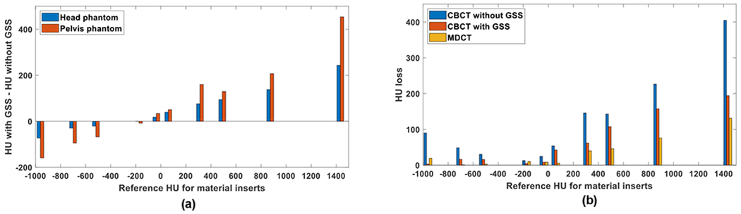
For example, for the cortical bone insert in the Gammex head phantom (red arrow in Fig. 9), values increased by 244 HU after residual scatter correction. For the same material, the increase was 454 HU in the pelvis phantom (Fig. 11(a)). In addition, scatter-induced artifacts between high density materials were reduced significantly after residual scatter correction.

The change in HU was less in water-equivalent background than bone-like materials; after residual scatter correction, HU values increased by 25 and 34 HU on the average in head and pelvis phantoms, respectively. Such material and object size dependent changes in HU values are expected, since scatter-to-primary ratio is higher in projections of high-density inserts (due to high primary attenuation) and larger objects.

To measure the degradation in HU values as function of phantom size, an HU loss metric was calculated (Fig. 11(b), Table II). In images acquired with 2D grid only, HU loss was in the range of 30-405 HU for the Gammex phantom. After residual scatter correction, HU loss was reduced to a range of 16-194. In MDCT images, HU loss was in the range of 1-131. Similar trends were also observed in the Catphan phantom.

TABLE II.

HU loss metric in Gammex and Catphan phantoms

	Mean [min max] HU loss
	Gammex	Catphan
2D grid only	150 [30 405]	59 [13 148]
2D grid + GSS	85 [16 194]	20 [5 49]
MDCT	43[1 131]	11 [1 24]

CT number uniformity were also improved with scatter residual scatter correction (Table III). In the Gammex head phantom, HU uniformity was improved from 39 to 32 HU with GSS correction. In the pelvis phantom, HU uniformity was improved more than factor of two, from 65 to 30 HU with GSS correction. In MDCT images, uniformity was 12 and 21 HU for head and pelvis phantoms, respectively.

TABLE III.

HU nonuniformity in water-equivalent sections

	Maximum HU difference and standard deviation among nine ROIs
	Head		Pelvis
	Max difference	Standard deviation	Max difference	Standard deviation
2D grid only	39 HU	±12.3 HU	65 HU	±21.7 HU
2D grid + GSS	32 HU	±10.3 HU	30 HU	±10.2 HU
MDCT	12 HU	±4.7 HU	21 HU	± 6.4 HU

3.3. Effect of GSS method on noise, contrast, and CNR

Noise (K_noise) and contrast (K_contrast), and CNR (K_CNR) improvement factors were calculated in head and pelvis sized phantoms (Table IV). After residual scatter correction with GSS, noise increased by a factor a factor of 1.12 and 1.26 in Catphan head and pelvis phantoms. Larger increase in noise in pelvis phantom was expected, due to higher residual scatter intensity. Contrast also increased about the same amount due to recovery of contrast after scatter correction^1,2,40.

TABLE IV.

Noise (K_NOISE), Contrast (K_CONTRAST), and CNR (K_CNR) improvement factors after application of GSS

	Catphan (head)	Catphan (pelvis)	Gammex (head)	Gammex (pelvis)
Knoise	1.12±0.09	1.26±0.15	1.07±0.15	1.02±0.29
Kcontrast	1.12±0.09	1.27±0.04	1.08±0.09	1.31±0.03
KCNR	1.00±0.09	1.02±0.11	1.03±0.19	1.39±0.53

While similar trends were also observed in the Gammex phantom, the increase in noise after scatter correction was minimal in the pelvis phantom. This was due to significant reduction in image artifacts after scatter correction. While stochastic noise increases after scatter corrections, reduced image artifacts due to scatter correction reduce standard deviation of HU values.

After residual scatter correction, noise increased by 2-26% and contrast increased values increased by 8-31%. Hence, CNR improvement factors were close to 1 in both head and pelvis phantoms (Table IV). These results indicated that CNR was minimally affected by residual scatter correction. A slight increase of K_CNR in Gammex phantom after scatter correction was attributed to less than expected increase in image noise due to reduced image artifacts as described in the previous paragraph.

3.4. Effect of GSS method on grid induced ring artifacts

As illustrated in Fig. 3, pixel values in septal shadows were overcompensated by GM calibration data, when residual scatter is present. As a result, pixel values in septal shadows are higher than pixel values in adjacent grid holes, which led to ring artifacts in high resolution CBCT images (Fig. 13). Formation of grid line artifacts is demonstrated in two sets of phantom projections in Fig. 12. In raw projections (row (a)), hypointense septal shadows are clearly visible. After gain correction (row (b)), septal shadows are overcompensated due to presence of residual scatter, and hyperintense grid line artifacts are apparent. In row (c), residual scatter map calculated via GSS method is shown. After scatter map subtraction and gain correction, grid line artifacts diminish (row (d)). In CBCT images, ring artifacts reduced substantially after scatter correction (Fig. 13). Ring artifacts in the periphery of phantoms (blue arrow) were due to an issue associated with detector readout. Thus, they were not corrected by residual scatter correction. There were also faint ring artifacts in the center of the phantoms. While we did not determine the exact cause of these artifacts, they might be caused by uncorrected residual scatter, small but random deviations in gantry flex⁴¹, suboptimal gain correction due to detector lag and ghosting⁴², detector artifacts, and nonlinear pixel readout gain³².

Fig.13.

Effect of residual scatter correction on ring artifact reduction. ROIs outlined in red are displayed in the insets. High resolution reconstructions with 0.39 mm isotropic voxels. (a-b), Without the GSS method, residual scatter in projections caused ring artifacts in reconstructed images. (c-d), After correction of residual scatter with GSS, ring artifacts are suppressed. Line pairs indicated by the red arrow correspond to 1 line pair per mm. Artifacts in the periphery (blue arrow) were associated with detector readout, and therefore, it was not corrected. HU window (a, c): [−1000 2000] (b,d): [−500 500].

Fig. 12.

Projection images of the Catphan spatial resolution phantom (reconstructed images in Fig. 12) and pelvis sized Gammex electron density phantom (reconstructed images in Fig. 9). Only a zoomed in section of the Gammex phantom is shown, and hypointense object is the cortical bone insert. Row (a), raw projection: intensity reduction in 2D grid’s shadows is clearly visible. Row (b), flat-field corrected projection: Since residual scatter was not corrected, septal shadows are overcompensated, and appear as hyperintense lines. Row (c), scatter map: Residual scatter intensity as measured by the GSS method. Row (d), GSS Method: Residual scatter was subtracted from the raw projection, followed by flat-field correction.

Reduction of artifacts was also evident in image noise evaluations. Before residual scatter correction, noise in five uniform background ROIs in Fig. 13(b) was 103±39 HU, where standard deviation indicates the variation of noise among ROIs. After residual scatter correction in Fig. 13(d), noise was reduced to 61±6 HU, corresponding to 41% reduction in noise.

It is important to note that ring artifacts are not prominent in images shown in Figs. 7 and 8 because of larger voxel size (0.9x0.9x1 mm³). Images in Fig. 13 have smaller 0.39 mm isotropic voxels that preserved high spatial frequency artifacts.

Since ring artifact reduction was achieved by subtracting a spatially smooth scatter map, the spatial resolution was not degraded in CBCT images. Preservation of spatial resolution was discernible in the line pair phantom images (Figs. 13 (a), (c)). Bar pattern for one line-pair/mm (lp/mm) could be resolved with and without residual scatter correction. MTF curves calculated with and without scatter correction were also similar (Fig. 14), which supported our qualitative observations. MTF value of 0.1 corresponded to one lp/mm, which was in agreement with the resolution observed in the line pair phantom. While small differences between the two MTF curves exist, these were attributed to ring artifacts in the image reconstructed without residual scatter correction.

Fig. 14.

The effect of GSS method on the MTF in CBCT images.

4. Discussion

In this work, we have presented a new scatter suppression method which unifies scatter rejection and measurement-based scatter correction in CBCT. Our method, referred to as grid-based scatter sampling, utilizes 2D antiscatter grid hardware both for scatter rejection and scatter correction. Our preliminary results indicate that significantly higher CT number consistency, approaching that of MDCT images, can be achieved in CBCT images.

Accurate, measurement-based scatter correction methods are considered challenging to implement in clinical CBCT systems, partly due to increased electromechanical complexity. Our GSS method addresses the shortcomings of measurement-based scatter correction, and may enable clinical implementation due to following: since the 2D grid itself acts as the scatter measurement device, it eliminates the need for an additional device for scatter measurement, such as a beam-stop or a fluence modulation array ^3,5. Besides increasing electromechanical complexity of the imaging system, the latter devices are more challenging to use in clinical CBCT systems because these exhibit gantry flex. During a CBCT scan, source position fluctuates with respect to detector due to gantry flex, and projection position of the beam-stop or modulator array also varies. Since beam stops and modulator arrays must be placed close to the x-ray source, errors in their projection positions are naturally magnified at the detector plane. These positioning errors reduce the fidelity of the calibration data, such as the expected location of beam stops on the detector plane. Consequently, accuracy of scatter measurements may be reduced, and new image artifacts may be introduced. In contrast, the 2D grid is placed directly on the detector in our approach, and magnification of positioning errors is considerably diminished. While placement of 2D grid on the detector reduces errors due to gantry flex, it does not eliminate the effects of gantry flex. To further reduce the detrimental effects of gantry flex, we employ gantry angle specific gain calibration²⁶. Our method also eliminates the need for acquisition of redundant image data for scatter measurements, which can potentially reduce imaging dose.

While model-based scatter correction approaches^1,2 can also be used in conjunction with 2D grids to correct residual scatter, our GSS method has fundamental advantages. Firstly, model-based methods rely on an object model for estimation of scatter distribution. In such models, ground truth object properties, such as material composition, are not known, and must be approximated. Object truncation in axial images, and temporal variations, such as breathing motion, will not be correctly represented in a stationary 3D model. Such differences between ground-truth and approximated object properties can lead to under- over- estimation of scatter intensity. Secondly, scatter rejection properties of the 2D grid must be explicitly modeled. Based on our experience ²⁵, simplified models for the grid, such as constant scatter transmission fraction, will not correctly depict transmission properties of a 2D grid. We emphasize that GSS makes no assumptions about the imaged object, eliminating the need for a grid transmission model.

After scatter correction with GSS, both noise and contrast increased by about the same magnitude, and CNR remained approximately constant. Subtraction of smooth scatter intensity maps in projections increases noise and contrast by the same amount, and this CNR remains the same. While we observed a slight increase in CNR after GSS correction, this is largely due to reduction of artifacts, and its effect on noise calculations used in CNR.

For the imaging conditions tested in this work, there was no reduction in CNR after scatter correction. However, a common challenge with subtraction-based scatter correction methods is that CNR and tissue visualization in reconstructed images might be reduced. Such a degradation in CNR is expected when effects of scatter vary as a function of projection view angle¹. However, CNR is expected to be preserved after scatter correction for rotationally symmetric conditions, such that effects of scatter do not vary as a function of projection view angle¹. Therefore, the change in CNR after scatter correction is likely task- and object-dependent and additional adaptive noise reduction strategies might be required.

Even though CT number consistency in CBCT images was improved substantially after residual scatter correction, MDCT images still showed more consistent CT numbers than CBCT images. This is attributed to other effects contributing to HU degradation, such as beam hardening and incomplete sampling in cone beam geometry, which were not accounted for in the CBCT reconstructions presented in this work. Correction for beam hardening, image lag and other effects, which will be addressed in future work, is expected to further improve the CT number accuracy in CBCT images.

Grid-induced image artifacts are a major challenge in translation of 2D grids into clinical flat panel detector based CBCT systems. Our work demonstrates that residual scatter is a major cause of such image artifacts. By correcting for residual scatter, the GSS method reduces image artifacts while preserving spatial resolution.

As an alternative to the GSS method, residual scatter can be reduced by improving the scatter rejection performance of 2D grids. However, this approach requires increasing the grid ratio, which may cause problems in grid-source alignment, challenges in fabrication, and increase manufacturing costs. Residual scatter correction via GSS method achieves high CT number accuracy at lower grid ratios, permitting more flexibility in grid design.

An important assumption in the GSS is that scatter intensity is uniform in a neighborhood of pixels consisting of septal shadows and holes. This assumption might be considered counterintuitive, since a 2D grid is placed between the patient and the detector, and scatter fluence (like primary) is expected to be reduced in grid’s shadows. However, such a reduction in scatter is minimal for two reasons: (a) the grid septa in our design are purposely thin (~ 0.1 mm), and (b) a deliberate air gap between the grid and the detector is designed to allow a broader angle distribution of scatter fluence to reach the septal shadows in the detector plane.

Since the residual scatter signal is relatively low in projections (majority of scatter is rejected the 2D grid), noise due to low signal intensity may introduce errors during scatter estimation. Low detector entrance exposure conditions, such as large imaged object size, highly attenuating material compositions, or low tube current, may further increase noise and affect accuracy of scatter estimation. Furthermore, high grid ratio 2D grids reduce residual scatter intensity and may challenge accurate scatter estimation. The performance of the GSS method under low detector entrance exposure conditions remains to be investigated.

The GSS method achieves primary intensity modulation by fully blocking primary x-rays incident on the grid septa. Given that the height of the tungsten septa are approximately 20 mm ^23,25, these will continue to fully block primary x-rays in the orthovoltage range. Even though scatter rejection performance of the grid will deteriorate at orthovoltage energies, increased residual scatter intensity can be corrected by using the GSS method.

5. Conclusion

The GSS method proposed in this work achieved both robust scatter rejection and scatter correction, by extending the role of 2D antiscatter grid to scatter measurement in flat detector based CBCT. This unified approach not only provides higher CT number accuracy, but also suppresses grid-induced artifacts in CBCT, which has previously challenged the translation of 2D grids into clinical CBCT systems. This approach inherently preserves spatial resolution, providing a significant advantage over conventional ring artifact suppression methods.

Improved CT number accuracy may open the path to new applications in CBCT imaging. For example, dual energy CBCT is currently limited to small objects in part due to poor CT number accuracy. CBCT-based radiation therapy dose calculations, extraction of radiomics features, and image classification and diagnosis using machine learning methods are also challenging to implement. Thus, higher CT number accuracy may accelerate clinical utilization of these methods. The GSS method can potentially be employed in higher x-ray energy imaging beyond the diagnostic energy range. Therefore, the utility of our 2D grid design and GSS method may be extended into industrial and security imaging applications that employ orthovoltage or higher x-ray energies.

References

- 1.Ruhrnschopf E-P, Klingenbeck K. A general framework and review of scatter correction methods in x-ray cone-beam computerized tomography. Part 1: Scatter compensation approaches. Medical Physics. 2011;38(7):4296–4311. [DOI] [PubMed] [Google Scholar]
- 2.Ruhrnschopf E-P, Klingenbeck aK. A general framework and review of scatter correction methods in cone beam CT. Part 2: Scatter estimation approaches. Medical Physics. 2011;38(9):5186–5199. [DOI] [PubMed] [Google Scholar]
- 3.Ning R, Tang X, Conover DL. X-ray scatter suppression algorithm for cone-beam volume CT. Proc SPIE. 2002;4682:774–781. [Google Scholar]
- 4.Liu X, Shaw CC, Wang T, Chen L, Altunbas MC, Kappadath SC. An accurate scatter measurement and correction technique for cone beam breast CT imaging using scanning sampled measurement (SSM)technique. Proc SPIE. 2006;6142:614234. [DOI] [PMC free article] [PubMed] [Google Scholar]
- 5.Zhu L, Strobel N, Fahrig R. X-ray scatter correction for cone-beam CT using moving blocker array. 2005. [Google Scholar]
- 6.Niu T, Zhu L. Single-scan scatter correction for cone-beam CT using a stationary beam blocker: a preliminary study. 2011. [DOI] [PMC free article] [PubMed] [Google Scholar]
- 7.Liang X, Jiang Y, Zhao W, et al. Scatter correction for a clinical cone-beam CT system using an optimized stationary beam blocker in a single scan. Medical physics. 2019;46(7):3165–3179. [DOI] [PubMed] [Google Scholar]
- 8.Parker DL. Optimal short scan convolution reconstruction for fan beam CT. Medical physics. 1982;9(2):254–257. [DOI] [PubMed] [Google Scholar]
- 9.Wang G X-ray micro-CT with a displaced detector array. Medical physics. 2002;29(7):1634–1636. [DOI] [PubMed] [Google Scholar]
- 10.Doi K, Fujita H, Ohara K, et al. Digital radiographic imaging system with multiple-slit scanning x-ray beam: preliminary report. Radiology. 1986;161(2):513–518. [DOI] [PubMed] [Google Scholar]
- 11.Ren L, Yin FF, Chetty IJ, Jaffray DA, Jin JY. Feasibility study of a synchronized-moving-grid (SMOG) system to improve image quality in cone-beam computed tomography (CBCT). Medical physics. 2012;39(8):5099–5110. [DOI] [PubMed] [Google Scholar]
- 12.Jin JY, Ren L, Liu Q, et al. Combining scatter reduction and correction to improve image quality in cone-beam computed tomography (CBCT). Medical physics. 2010;37(11):5634–5644. [DOI] [PubMed] [Google Scholar]
- 13.Wang J, Mao W, Solberg T. Scatter correction for cone-beam computed tomography using moving blocker strips: A preliminary study. Medical Physics. 2010;37(11):5792–5800. [DOI] [PubMed] [Google Scholar]
- 14.Altunbas M, Shaw C, Liu X, et al. MO-E-L100J-06: Slot Scan Imaging with a High Frame Rate Flat Panel Detector-Measurement and Correction for In-Slot Scatter. Medical Physics. 2007;34(6Part16):2527–2527. [Google Scholar]
- 15.Liu X, Shaw CC, Altunbas MC, Tianpeng W. An alternate line erasure and readout (ALER) method for implementing slot-scan imaging technique with a flat-panel detector-initial experiences. Medical Imaging, IEEE Transactions on. 2006;25(4):496–502. [DOI] [PMC free article] [PubMed] [Google Scholar]
- 16.Zhu L, Bennett NR, Fahrig R. Scatter correction method for X-ray CT using primary modulation: theory and preliminary results [published online ahead of print 2006/12/16]. IEEE transactions on medical imaging. 2006;25(12):1573–1587. [DOI] [PubMed] [Google Scholar]
- 17.Zhu L, Gao H, Bennett NR, Xing L, Fahrig R. Scatter correction for x-ray conebeam CT using one-dimensional primary modulation. 2009. [Google Scholar]
- 18.Gao H, Zhu L, Fahrig R. Optimization of system parameters for modulator design in x-ray scatter correction using primary modulation. 2010. [DOI] [PMC free article] [PubMed] [Google Scholar]
- 19.Hsieh S Estimating scatter in cone beam CT with striped ratio grids: A preliminary investigation. Medical physics. 2016;43(9):5084–5092. [DOI] [PubMed] [Google Scholar]
- 20.Hsieh SS, Wang AS, Star-Lack J. Striped ratio grids for scatter estimation. Paper presented at: Medical Imaging 2016: Physics of Medical Imaging 2016. [Google Scholar]
- 21.Nagesh SS, Rana R, Bednarek D, Rudin S. Anti-scatter grid artifact elimination for high-resolution x-ray imaging detectors without a prior scatter distribution profile. Paper presented at: Medical Imaging 2018: Physics of Medical Imaging 2018. [DOI] [PMC free article] [PubMed] [Google Scholar]
- 22.Altunbas C, Zhong Y, Shaw CC. Feasibility of 2D antiscatter grid concept for flat panel detectors: preliminary investigation of primary transmission properties. arXiv preprint arXiv:200804271. 2020. [Google Scholar]
- 23.Altunbas C, Kavanagh B, Alexeev T, Miften M. Transmission characteristics of a two dimensional antiscatter grid prototype for CBCT. Medical physics. 2017;44(8):3952–3964. [DOI] [PMC free article] [PubMed] [Google Scholar]
- 24.Fetterly KA, Schueler BA. Physical evaluation of prototype high-performance anti-scatter grids: potential for improved digital radiographic image quality [published online ahead of print 2008/12/23]. Phys Med Biol. 2009;54(2):N37–42. [DOI] [PubMed] [Google Scholar]
- 25.Altunbas C, Alexeev T, Miften M, Kavanagh B. Effect of grid geometry on the transmission properties of 2D grids for flat detectors in CBCT. Physics in Medicine & Biology. 2019;64(22):225006. [DOI] [PMC free article] [PubMed] [Google Scholar]
- 26.Alexeev T, Kavanagh B, Miften M, Altunbas C. Two-dimensional antiscatter grid: A novel scatter rejection device for Cone-beam computed tomography. Medical physics. 2018;45(2):529–534. [DOI] [PMC free article] [PubMed] [Google Scholar]
- 27.Zbijewski W, Gang GJ, Xu J, et al. Dual-energy cone-beam CT with a flat-panel detector: Effect of reconstruction algorithm on material classification. Medical Physics. 2014;41(2):-. [DOI] [PMC free article] [PubMed] [Google Scholar]
- 28.Shi L, Bennett NR, Shapiro E, et al. Comparative study of dual energy cone-beam CT using a dual-layer detector and kVp switching for material decomposition. Vol 11312:SPIE; 2020. [DOI] [PMC free article] [PubMed] [Google Scholar]
- 29.Schmidt TG. CT energy weighting in the presence of scatter and limited energy resolution. Medical physics. 2010;37(3):1056–1067. [DOI] [PubMed] [Google Scholar]
- 30.Rana R, Jain A, Shankar A, Bednarek D, Rudin S. Scatter estimation and removal of anti-scatter grid-line artifacts from anthropomorphic head phantom images taken with a high resolution image detector. Paper presented at: Medical Imaging 2016: Physics of Medical Imaging 2016. [DOI] [PMC free article] [PubMed] [Google Scholar]
- 31.Seibert JA, Boone JM, Lindfors KK. Flat-field correction technique for digital detectors. Proc SPIE. 1998;3336:348–354. [Google Scholar]
- 32.Altunbas C, Lai C-J, Zhong Y, Shaw CC. Reduction of ring artifacts in CBCT: Detection and correction of pixel gain variations in flat panel detectors. Medical physics. 2014;41(9):091913. [DOI] [PubMed] [Google Scholar]
- 33.Feldkamp L, Davis L, Kress J. Practical cone-beam algorithm. Journal of the Optical Society of America a-Optics Image Science and Vision. 1984;1(6):612–619. [Google Scholar]
- 34.Biguri A, Dosanjh M, Hancock S, Soleimani M. TIGRE: a MATLAB-GPU toolbox for CBCT image reconstruction. Biomedical Physics & Engineering Express. 2016;2(5):055010. [Google Scholar]
- 35.Agostinelli S, Allison J, Amako Ka, et al. GEANT4—a simulation toolkit. Nuclear instruments and methods in physics research section A: Accelerators, Spectrometers, Detectors and Associated Equipment. 2003;506(3):250–303. [Google Scholar]
- 36.Allison J, Amako K, Apostolakis J, et al. Recent developments in Geant4. Nuclear Instruments and Methods in Physics Research Section A: Accelerators, Spectrometers, Detectors and Associated Equipment. 2016;835:186–225. [Google Scholar]
- 37.Wang A, Maslowski A, Messmer P, et al. Acuros CTS: A fast, linear Boltzmann transport equation solver for computed tomography scatter–Part II: System modeling, scatter correction, and optimization. Medical physics. 2018;45(5):1914–1925. [DOI] [PubMed] [Google Scholar]
- 38.Schafer S, Stayman JW, Zbijewski W, Schmidgunst C, Kleinszig G, Siewerdsen JH. Antiscatter grids in mobile C-arm cone-beam CT: Effect on image quality and dose. Medical Physics. 2012;39(1):153–159. [DOI] [PMC free article] [PubMed] [Google Scholar]
- 39.Friedman SN, Fung GS, Siewerdsen JH, Tsui BM. A simple approach to measure computed tomography (CT) modulation transfer function (MTF) and noise-power spectrum (NPS) using the American College of Radiology (ACR) accreditation phantom. Medical physics. 2013;40(5):051907. [DOI] [PMC free article] [PubMed] [Google Scholar]
- 40.Altunbas C Image corrections for scattered radiation. In: Shaw CC, ed. Cone Beam Computed Tomography. Boca Raton, FL: CRC Press; 2014:129–147. [Google Scholar]
- 41.Sharpe MB, Moseley DJ, Purdie TG, Islam M, Siewerdsen JH, Jaffray DA. The stability of mechanical calibration for a kV cone beam computed tomography system integrated with linear acceleratora). Medical Physics. 2006;33(1):136–144. [DOI] [PubMed] [Google Scholar]
- 42.Siewerdsen JH, Jaffray DA. A ghost story: Spatio-temporal response characteristics of an indirect-detection flat-panel imager. Medical Physics. 1999;26(8):1624–1641. [DOI] [PubMed] [Google Scholar]