Is the Rise in Illicit Opioids Affecting Labor Supply and Disability Claiming Rates?

Abstract

This paper examines how the recent transition of the opioid crisis from prescription opioids to more prevalent misuse of illicit opioids, such as heroin and fentanyl, altered labor supply behavior and disability insurance claiming rates. We exploit differential geographic exposure to the reformulation of OxyContin, the largest reduction in access to abusable prescription opioids to date, to study the effects of substitution to illicit markets. We observe meaningful reductions in labor supply measured in terms of employment-to-population ratios, hours worked, and earnings in states more exposed to reformulation relative to those less exposed. We also find evidence of increases in disability applications and beneficiaries.

1. Introduction

The opioid crisis in the United States is a national emergency. In 2017 alone, more than 70,000 individuals died of drug overdoses; almost 70% involved opioids (Scholl et al., 2019). There is widespread interest in understanding the broader effects of the opioid crisis beyond overdoses. In particular, policymakers and researchers have expressed concern about its economic consequences and its implications for labor markets and social insurance programs.¹ There is evidence that the link between the crisis and the labor market may be especially strong, and the Federal Reserve Chairman Jerome Powell maintained that the opioid crisis is having a “substantial” effect on the United States economy.²

Complicating efforts to quantify the broader effects of the opioid crisis, the epidemic continues to evolve. Before 2010, the “first wave” was driven primarily by misuse of natural and semi-synthetic opioids, such as OxyContin. In 2010, a pivotal transformation produced a second wave, a heroin epidemic, which transitioned in 2013 into the third wave–an illicit fentanyl crisis. These waves can be observed in fatal overdose trends by opioid type, which are presented in Figure 1. Recent research suggests that the transformation from prescription to illicitly-manufactured opioids was driven by the reformulation of OxyContin. In 2010, Purdue Pharma introduced an abuse-deterrent version of OxyContin, replacing the original formulation. This replacement represented a substantial shock to the availability of abusable prescription opioids as OxyContin was often the “drug of choice” for non-medical users (Cicero et al., 2005). Prior research has shown that states with higher rates of non-medical use of OxyContin experienced disproportionate growth in heroin overdose rates after reformulation (Alpert et al., 2018). In recent years, widespread substitution to illicit opioids has only increased in importance (Pardo et al., 2019), leading to disproportionately fast growth in overdose death rates in states more exposed to reformulation (Powell and Pacula, 2021).

Figure 1: National Fatal Overdose Rate Trends.

Notes: Figure 1 plots national annual fatal overdose rate trends in natural and semi-synthetic opioids (T40.2), heroin (T40.1), and synthetic opioids (T40.4) per 100,000 people for 1999-2017. These categories are not mutually exclusive and sum to rates higher than the overall opioid overdose rate. OxyContin is a semi-synthetic opioid.

Source: National Vital Statistics System

A small, but growing, literature empirically analyzes how prescription opioid availability and overprescribing affect the labor market. Focusing on the overprescribing dimension, Harris et al. (2019) find that areas with more high-volume prescribers have lower labor force participation rates. Krueger (2017) and Aliprantis et al. (2019) suggest that the rise in opioid prescribing since 2000 can explain a meaningful share of the decline in labor force participation over that time period, comparing labor supply changes in areas with faster growth in opioid supply to those with lower growth. Currie et al. (2019) and Savych et al. (2019) also study geographic variation in measures of prescribing behavior over time. It is rare in this literature to leverage policy-driven variation. A recent exception is Beheshti (2019), who exploits the differential geographic impacts of the rescheduling of hydrocodone, finding convincing evidence that reduced medical access to hydrocodone improved labor force participation rates.

To date, the literature on the labor supply impacts of the opioid crisis measures opioid exposure in terms of geographic prescribing rates and legal opioid supply. In contrast, this paper examines the labor supply and disability insurance effects of the transition from prescription opioids to illicit opioids, drugs that are not measured in prescriptions. This perspective is perhaps more relevant to the current state of the epidemic given that the opioid crisis continues to escalate despite a 60% drop in prescription opioid volume in the United States since 2011 (IQVIA Institute, 2020). More broadly, it is rare to study the labor supply and social insurance consequences of a large shock to the size of illicit drug markets.³

We analyze how the reformulation of OxyContin affected labor market outcomes and applications for disability benefits. As the supply of abusable prescriptions opioids decreased, people switched to illicit markets and these markets grew disproportionately in areas where OxyContin misuse had been more prevalent (Powell and Pacula, 2021). Given evidence that OxyContin reformulation transformed the opioid crisis, it is important to understand how that transformation affected social insurance programs and the labor market. Estimates of the productivity costs of illicit drug use in the literature are large. Jiang et al. (2017) conclude that heroin use disorder alone in the United States results in over $5 billion of productivity losses annually. In addition, a host of papers have explored the association between personal drug use and labor supply outcomes (e.g., Kaestner, 1994; Zarkin et al., 1998; MacDonald and Pudney, 2000; French et al., 2001; DeSimone, 2002) or used policy variation to identify this relationship (e.g., Nicholas and Maclean, 2019; Sabia and Nguyen, 2018). We explore the direction and magnitude of effects from a broad market-wide shift from prescription opioids to illicit opioids.

There is also interest in understanding the broader effects of supply-side interventions designed to deter opioid misuse, and a small literature has documented possible labor supply effects of prescription drug monitoring programs (PDMPs) (Kilby, 2015; Franco et al., 2019; Deiana and Giua, 2018; Kaestner and Ziedan, 2020). This paper also intersects with the literature studying the labor supply consequences of access to prescription drugs. Prior research found evidence that access to Cox-2 inhibitors increased labor force participation in the United States (Garthwaite, 2012) and decreased sickness absences in Norway (Bütikofer and Skira, 2018). We study the removal of an abusable formulation of a pain management therapy when more dangerous pharmacological substitutes are available illicitly.

We use several complementary data sets to document labor supply outcomes including data from the Bureau of Economic Analysis (BEA), Current Employment Statistics (CES), and the American Community Survey (ACS) to construct measures of labor supply such as the employment rate, hours worked, and earnings. We also rely on administrative data from the Social Security Administration (SSA) concerning applications and allowances for disability benefits through Social Security Disability Insurance (SSDI) and Supplemental Security Income (SSI). We study these disability-related measures for two reasons. First, misuse of medical and illicit opioids may put people at risk of permanently reducing labor supply, making disability insurance applications and allowances useful proxies for longer-term labor force attachment in this context.

Second, there is significant policy interest in what drives increases in disability insurance applications and enrollment, especially when these mechanisms are not more traditional factors predicting disability enrollment such as demographic shifts. At $143 billion, SSDI represents 4% of the federal budget.⁴ Several papers have found that worsening local economic conditions predict increases in disability payments (Autor and Duggan, 2003; Black et al. 2002; Autor et al., 2013; Charles et al., 2018; Maestas et al., 2018). However, there is little work exploring how the growth of illicit drug markets affects enrollment in disability insurance programs.

At an individual level, substitution from OxyContin to heroin or fentanyl could affect an individual’s ability to function in the labor force given the additional potency of illicit opioids and the associated health risks (e.g., due to higher rates of injection use). In addition, acquiring heroin may introduce individuals to illicit markets, which could have independent harmful consequences such as exposing them to criminal behavior or increasing risk of victimization. Heroin use – relative to prescription opioid misuse – could also increase the propensity to fail drug tests, hurting employment prospects. On the other hand, if reformulation induced some to stop misusing opioids entirely⁵ or reduced rates of initiation into opioid misuse, then we may observe beneficial outcomes.

At the market level, a broad transition from prescription opioids to heroin may cause illicit drug markets to expand beyond individuals previously misusing OxyContin. Drug market expansion could alter labor markets with general equilibrium ramifications on employment, induce crime, and systematically change population health. In the end, it is difficult to predict the effects of such a dramatic shift from prescription to illicit drugs since there is little evidence about what such an enormous transition will do to individual-and market-level behaviors.

We study changes in labor supply and disability outcomes in states with higher rates of OxyContin misuse before OxyContin reformulation relative to those with lower rates. Reformulation impacted the supply of abusable opioids nationally, but we exploit that states with higher rates of OxyContin misuse were more exposed to the effects of reformulation, comparing more exposed to less exposed states. Our primary empirical strategy transparently traces the relationship between OxyContin misuse and these outcomes in each year, conditioning on state and time fixed effects, while also accounting for the independent effects of pre-reformulation rates of pain reliever misuse more generally.

We observe large effects on labor supply and disability claiming. We estimate reductions in employment-to-population ratios in multiple data sets, beginning at the time of reformulation and growing over time. Additionally, we estimate even larger proportional reductions in hours worked, full-time work, earnings, and total employee compensation, suggesting important “intensive margin” effects as well. Moreover, the reductions in employment and full-time work are associated with decreases in health insurance rates. Our results also suggest that reformulation induced more people to apply for disability benefits, and many of these individuals met the SSA’s disability criteria and eventually received disability benefits. We estimate increases in disability applications, favorable determinations, and total beneficiaries. The differential rise in disability applications begins immediately after reformulation, and there is little evidence of any systematic pre-existing trends (or even level differences). The evidence is consistent with reformulation as the driving mechanism and not other policies or confounding factors resulting from the Great Recession.

Our results imply that a state with a one standard deviation higher rate of non-medical OxyContin use prior to reformulation experienced a 7% relative increase in disability applications after reformulation. A back-of-the-envelope calculation suggests that the labor supply impacts of growth in illicit opioid markets are comparable to, but on the lower end of the distribution of estimated effects of, the consequences of legal opioid access increases found in the literature.

Although substance use disorders alone cannot be used as qualifying conditions for disability benefits, these results suggest that growth in illicit drug markets alters the labor market capabilities of those with other disabling conditions and/or worsens economic conditions for this population. The literature has provided evidence that economic conditions can drive application rates and alter the size of disability insurance rolls. This paper demonstrates that general equilibrium shocks to illicit drug markets can also affect demand for disability benefits.

We discuss these interactions further in the next section while also providing background on the reformulation of OxyContin. We describe the data used in the analysis in Section 3, and our empirical strategy in Section 4. We present our results in Section 5 and discuss our conclusions in Section 6.

2. Background

2.1. Disability Insurance in the United States

The Social Security Disability Insurance (SSDI) and Supplemental Security Income (SSI) programs are the largest federal programs providing monetary and non-monetary support – such as health insurance – to people with disabilities in the United States. In December 2017, 12.7 million people ages 18-64 received disability benefits – 62% received SSDI benefits only, 28% received SSI benefits only, and 10% received benefits from both SSDI and SSI.⁶ SSDI is generally available to individuals with a sufficient work history while SSI is intended primarily for individuals with little work experience and is subject to asset thresholds.⁷

When it began in 1956, SSDI provided benefits to people with disabling conditions, including those unable to work because of substance use disorders. SSI, introduced in the Social Security Amendments of 1972, defined disabling conditions using similar guidelines. However, with the introduction in 1997 of public law 104-121, substance use disorder beneficiaries became disqualified unless they also qualified under other disability requirements (Gresenz et al., 1998).⁸ Since substance use does not disqualify individuals from receiving benefits, it may increase application rates if the substance use exacerbates other disabilities or reduces labor market opportunities. Brucker (2007) estimates that a “substantial portion” of SSI/SSDI beneficiaries struggle with substance abuse, at rates much higher than the general population for drugs, suggesting considerable scope for large transitions in substance use to affect claiming rates.

The SSA outlines several ways in which substance use may appropriately lead to higher allowance rates.⁹ For example, substance use may lead to a claimant acquiring a disabling impairment (e.g., contracting HIV through needle use) or it could cause permanent impairments (the SSA provides dementia and amnestic disorders as examples of such conditions), which qualify claimants for disability benefits. Alternatively, there is substantial heterogeneity in the judgment of disability examiners (Maestas et al., 2013) and substance use may add variability to this decision process, potentially altering allowance rates.

Similarly, shocks to the prevalence of substance abuse could change disability claiming rates through increased demand (e.g., due to poorer individual labor market prospects or broader labor market conditions) to reduce labor supply. It is difficult to find exogenous shocks to illicit drug use so existing evidence is limited, and it is difficult to forecast these effects. One important exception in the literature is Maclean et al. (2019), who find that state medical marijuana laws increase disability insurance claiming rates.¹⁰

To apply for SSDI, an individual initially files an application at a Social Security office. The office screens applications to determine if an individual meets basic requirements such as age and work credits for Social Security disability benefits. If these conditions are met, then the application is reviewed by state Disability Determination Services to determine whether the individual is disabled under Social Security guidelines and unable to work. Denials can be appealed. Individuals who are approved receive cash benefits, which are a function of prior earnings, and access to health insurance through Medicare. The process for SSI is similar, though the eligibility requirements regarding work history and asset requirements are different. Monthly SSI payments are based on a federal benefit rate, and medical coverage is typically provided through State Medicaid programs.

Disability benefit receipt and labor supply are not mutually exclusive. While receiving disability benefits causally reduces earnings (Maestas et al., 2013; French and Song, 2014), many recipients still work. SSDI recipients are restricted to earn less than “substantial gainful activity” (SGA), equal to $1,260 per month ($2,110 for blind applicants), though there are exceptions to this rule and earning above this threshold is permitted for certain periods of time.

2.2. OxyContin Reformulation

OxyContin was introduced in 1996 by Purdue Pharma. It is a brand-name drug for the extended-release formulation of oxycodone, a semi-synthetic opioid, similar to morphine, used for the management of acute and chronic pain. The key innovation of OxyContin was its long-acting formula, which provided 12 hours of continuous pain relief, significantly improving the quality and ease of pain management compared to previous drugs. However, crushing or dissolving the pill caused the complete dose of oxycodone to be delivered immediately, making OxyContin especially easy to abuse.

OxyContin had more than $3 billion in sales in 2010, making it one of the highest selling drugs in the United States (Bartholow, 2011). It was also one of the leading drugs of abuse (Cicero et al., 2005). Many experts have implicated OxyContin as a key driver of the opioid epidemic (e.g., Kolodny et al., 2015) and recent work concludes that its introduction explains a significant share of the growth in overdoses since 1996 (Alpert et al., 2019).

In April 2010, Purdue Pharma introduced a reformulated version of OxyContin designed to make the drug more difficult to abuse. The abuse-deterrent version uses physicochemical barriers to make the pill hard to break, crush, or dissolve. The change increased the costs of misusing OxyContin while maintaining the medical benefits of the drug. The reformulated version can still be abused orally (i.e., taking higher doses than prescribed) and some users have found ways to counteract the abuse-deterrent properties of the new version.¹¹ However, reformulation has been shown to decrease abuse rates. In August 2010, Purdue Pharma stopped distributing the original formulation of OxyContin to pharmacies.

Recent research has shown that replacing the original formulation with the abuse-deterrent version increased heroin overdose rates (Alpert et al., 2018; Evans et al., 2019), heroin-specific substance abuse treatment admissions (Alpert et al., 2018), rates of infectious diseases (Powell et al., 2019; Beheshti, 2019), and illicit opioid crimes (Mallatt, 2020).¹² Instead of just shifting the exposed population from prescription opioid overdoses to illicit opioid overdoses, Powell and Pacula (2021) find that reformulation, over a longer time horizon, drastically increased overdose rates. While initially there was possibly just a shift to illicit markets, this shift caused those markets to grow and innovate over time.

While it is difficult to observe the number of consumers in illicit drug markets,¹³ Powell and Pacula (2021) find that exposure to reformulation is associated with increases in substance use treatment admissions for heroin (and opioids more broadly). This relationship is stronger for those without any prior treatment episodes, suggesting an increase in initiation into dependence even in recent years. In addition, this work ties reformulation to growth in non-opioid overdose deaths, such as cocaine, which is also consistent with exposure to potent illicit opioids among a new population. Overall, the evidence suggests substantial market expansion due to reformulation.

Similarly, in this paper, we are not isolating the labor supply effects of reformulation on those misusing OxyContin prior to reformulation. Instead, we study geographic effects, which include the expansion of illicit markets and its broader economic consequences. These general equilibrium effects are potentially larger than individual-level effects.

3. Data

We conduct our analyses at the state level given that the availability of data sources. We are specifically constrained by the measure of exposure to reformulation, which we only have at the state-level.¹⁴ While state boundaries likely do not appropriately define prescription or illicit drug markets, performing the analysis at the state-level should not induce bias. Aggregating to the state level is not problematic except for the loss of power, which is reflected in our standard errors. We select on 2001-2015 since all data sources are available for these years.

3.1. Labor Outcomes

We study multiple complementary measures of labor supply. First, we rely on data from the Bureau of Economic Analysis (BEA).¹⁵ The BEA provides state-level annual employment figures using data from the Current Employment Statistics (CES), discussed below, while adding information on employment in industries excluded from the CES (e.g., agriculture). The BEA also collects information from Internal Revenue Service data to estimate sole proprietorships and nonfarm partners such that the final employment numbers include the self-employed. We also study industry-specific effects using BEA employment figures.

We also use the BEA’s measure of employee compensation. Total employee compensation provides an additional measure of labor which nests a host of individual and firm-level decisions such as hours worked and occupational choice. The BEA compensation metric includes wages and salaries as well as the value of noncash benefits (e.g., employer contributions to health insurance and pension plans).¹⁶

We also study employment rates constructed using the CES data. The CES is a survey of establishments representing workers covered by unemployment insurance. Each month, the CES surveys about 145,000 nonfarm businesses and government agencies. By the nature of the survey design, the CES excludes some industries, such as agriculture, and the self-employed.

Both the BEA and CES are designed to provide employment totals based on place of work, not place of residence. We scale these employment figures by the total resident population ages 16 and above with the understanding that people may reside in one state and work in another. For both the BEA and CES, it is more accurate to refer to their employment numbers as the number of jobs since a person may have jobs at multiple establishments. However, we will generally refer to these variables as “employment rates” throughout this paper.

We also construct labor supply measures from the American Community Survey (ACS), an annual household survey.¹⁷ The ACS is self-reported, but we are able to construct labor outcomes by state of residence and study additional measures, such as usual hours worked per week.¹⁸ Usual hours per week is equal to zero for non-workers and, thus, incorporates both intensive and extensive labor supply behavior.

We also study earnings in the ACS, which we define as pre-tax wage and salary income plus self-employment income from businesses and farms.¹⁹ The annual labor outcomes in the ACS refer to the previous 12 months so we use the 2002-2016 samples to construct labor supply metrics for 2001-2015.²⁰ The ACS permit us to study labor effects based on demographics such as gender, age, race, and education. Overall, there are complementary benefits to each of these measures.

3.2. Disability Insurance Measures

To construct measures of disability claiming behavior, we use Social Security Administration (SSA) Fiscal Year Disability Claim Data, focusing on the adult population, defined as ages 18-64. These variables are available for fiscal years 2001-2015 at the state and annual level. We study the number of adult initial claims, which we will often refer to as applications for disability benefits though some applications are deemed ineligible in an initial screening and are never sent to a state agency. These applications are excluded from this measure. We divide the number of applications by the 18-64 population size. The data do not distinguish between SSI and SSDI benefits, but the majority of applicants in this age group are applying for SSDI.

We are also interested in whether these applicants eventually qualify for benefits. Public data provide the number of allowances in that year, regardless of when the initial applications were filed. Disability determinations often occur in a very short timeframe, but they can potentially take years. In such cases, some “post-reformulation” allowances would refer to applications filed prior to reformulation. By request, the SSA calculated and provided us with the “Total Allowances” (i.e., number of people approved for SSI or SSDI benefits) by state and year of application using data from the Disability Research File Reporting Service Cubes. Benchmarking each allowance to the initial year of the application is beneficial because we are interested in the downstream consequences on disability insurance enrollment for the changes in application rates that we observe.

The number of total allowances reflects people granted benefits whether their applications were initially approved or after one or more appeals. The number of total allowances could only be provided by calendar filing year. Because the number of applications are provided at the fiscal year (which ends in October) and the number of total allowances is provided at the calendar year, there is a slight misalignment when these measures are used together. For the more recent years of data, some of the applications are still pending: 5.8% of 2015 applications, decreasing to 1.7% for 2014 and less than 1% for all prior years.

We will also directly study the percentage of applicants approved for benefits, providing some evidence about the changing health of the applicants. The applicant pool may become less healthy because of the transition to illicit opioids, but the marginal applicants may also potentially be healthier on average. The net effect is an empirical question.

It is possible that state agencies alter their determination decisions in response to the changing environment. We cannot rule out this possibility, but the agents making these decisions have no incentive to modify their decision-making process due to economic conditions or changes in population health. We interpret our results about the fraction of applicants receiving favorable determinations as indicating changes in the health of the applicants, but we cannot empirically rule out systematic reviewer-side behavioral changes.

Finally, we study the fraction of the 18-64 population receiving disability benefits (as of December in each year), also provided in the SSA Fiscal Year Disability Claim Data. We highlight that changes in beneficiaries may reflect applications over, potentially, many years. Autor et al. (2015) report that for initial determinations, the median time to a decision is only three months. Thus, we would potentially expect to observe some evidence of immediate (i.e., 2010) effects if application rates quickly respond to reformulation given that most of these applications will receive decisions before the end of the year. However, there is additional scope for lagged effects for this outcome since cases which are initially denied may take years upon appeal before receiving a favorable determination.²¹

We also study the number of beneficiaries by diagnostic group. We collected these data from the Annual Statistical Reports on the Social Security Insurance Program (see Table 10 of those reports). These measures help provide some evidence about which conditions are affected by reformulation in terms of disability enrollment.

3.3. Nonmedical OxyContin and Pain Reliever Use

To measure non-medical use of OxyContin and pain relievers, we use state-level data from the NSDUH, a nationally representative household survey of individuals ages 12 and older and the country’s largest annual survey collecting information on substance use. The survey provides information on “non-medical OxyContin use” within the past year beginning in 2004 as well as “non-medical pain reliever use.” Alpert et al. (2018) found that non-medical OxyContin use was highly correlated with measures of oxycodone supply and OxyContin prescriptions. The advantage of this measure is that it specifies both “nonmedical use” and “OxyContin.” Substitution to illicit opioids should depend on the interaction of these two properties since OxyContin reformulation was specific to OxyContin and did not affect the medical capabilities of the drug.

Non-medical use is defined as use by individuals who either (a) were not originally prescribed the medication or (b) use such medications “only for the experience or feeling they caused.”²² Given the sensitive nature of pain reliever misuse, NSDUH provides respondents with a private and confidential way to respond to questions in an effort to increase honest reporting.²³ Nevertheless, self-reported data on drug use are subject to some under-reporting error. When constructing the nonmedical use variables, we combine the 2004-2009 surveys to reduce measurement error. We select these years because they precede the 2010 reformulation and are therefore untreated. Appendix Figure 1 provides a map of OxyContin misuse rates by state.

3.4. Summary Statistics

Figure 2 shows the time series trends in both the percentage of the 16+ population working and the percentage of the 18-64 population applying for disability benefits. There are large changes in both of these measures during the Great Recession, followed by partial convergence to pre-recession values by 2015.

Figure 2: National Time Series Trends in Percentage of Population Applying for Disability Insurance and Percentage Working.

Source: SSA Fiscal Year Disability Claims Data and Bureau of Economic Analysis. The percentage of disability applications is scaled by the 18-64 population while percentage working is the number of workers divided by the size of the 16+ population.

In Table 1, we provide summary statistics -- all dollar amounts in this paper are reported in 2015 dollars -- based on initial OxyContin misuse for 2004-2009, dividing the sample into “above median” and “below median” states. Alpert et al. (2018) showed that OxyContin misuse rates were uncorrelated with heroin overdose rates before reformulation. Similarly, we observe little difference in pre-reformulation labor or disability outcomes based on OxyContin misuse.

Table 1:

Summary Statistics for 2004-2009

Variable (2004-2009)	All States	Below Median OxyContin Misuse States	Above Median OxyContin Misuse States	Data Source
BEA Outcomes
% Employed	74.5%	74.4%	74.8%	BEA
Per Capita Employee Compensation ($)	37,144	38,270	34,567	BEA
CES Outcome
% Employed	57.4%	57.3%	57.4%	CES
ACS Outcomes
% Working	69.1%	69.2%	69.0%	ACS
Usual Hours Work Per Week	26.8	26.9	26.6	ACS
Annual Earnings ($)	27,412	28,140	25,747	ACS
Disability Insurance
% Apply	1.2%	1.1%	1.2%	SSA
% Favorable Determinations	0.6%	0.6%	0.6%	SSA
Favorable Determination Rate	49.6%	49.3%	50.4%	SSA
% Receiving Disability Benefits	5.5%	5.3%	6.0%	SSA
Demographics (%)
White, Non-Hispanic	67.0%	63.0%	76.3%	SEER
Hispanic	14.5%	16.3%	10.4%	SEER
Foreign-Born	19.2%	21.0%	15.1%	ACS
No High School Degree	13.5%	14.1%	12.2%	ACS
High School Graduate	28.9%	28.1%	30.6%	ACS
Some College	30.9%	30.5%	31.8%	ACS
Bachelor’s Degree (or more)	16.5%	27.2%	25.4%	ACS
Ages 18-24	15.8%	15.9%	15.7%	SEER
Ages 25-34	21.1%	21.4%	20.4%	SEER
Ages 35-44	22.7%	22.9%	22.4%	SEER
Ages 45-54	23.1%	22.9%	23.4%	SEER
Ages 55-64	17.2%	16.9%	18.1%	SEER
Misuse
OxyContin Misuse Rate (per 100)	0.57	0.45	0.84	NSDUH
Pain Reliever Misuse Rate (per 100)	4.88	4.61	5.51	NSDUH

Notes: All statistics are population-weighted. BEA, CES, and ACS outcomes scaled by 16+ population. Disability Insurance outcomes scaled by 18-64 population, except for Favorable Determination Rate (which is number of favorable determinations scaled by number of applications). All dollar amounts are expressed in 2015 dollars. BEA = Bureau of Economic Analysis; CES = Current Employment Statistics; ACS = American Community Survey; SSA refers to Social Security Administration data; SEER refers to population data from Surveillance, Epidemiology, and End Results Program; NSDUH = National Survey on Drug Use and Health. The SSA data are from the SSA Fiscal Year Disability Claim Data, the Disability Research File Reporting Service Cubes, or a calculation using both SSA data sets. Demographics are expressed as a percentage of the 18-64 population.

We also repeat Figure 2 but stratified based on initial OxyContin misuse rates. These can be seen in Appendix Figure 2. Both sets of states experienced large reductions in the percentage working due to the Great Recession. However, we observe stronger employment growth after reformulation in the low OxyContin misuse states, consistent with the main results below. Similarly, disability claiming falls much faster in low OxyContin misuse states after reformulation. Our event study analysis below more formally tests the appropriateness of these comparisons between high and low misuse states. Event studies help test for pre-existing trends; notably, according to Table 1, we also have similar pre-existing levels for most of the outcomes. This property is an important feature for difference-in-differences designs (Kahn-Lang and Lang, 2019) and reduces concerns about mean reversion as a potential driver of the estimated effects.

4. Empirical Strategy

We adopt an event study empirical design, which estimates the relationship between initial OxyContin misuse and labor/disability outcomes in each year, normalized to 0 in 2009. The specification is

$$Y_{\mathit{st}}={\alpha }_s+{\gamma }_t+{\delta }_t\times {\mathit{OxyRate}}_s^{\mathit{Pre}}+{\theta }_t\times {\mathit{PainRelieverRate}}_s^{\mathit{Pre}}+X_{\mathit{st}}^{\prime }\phi +{\epsilon }_{\mathit{st}},$$ (1)

where Y_st is a labor supply or disability outcome in state s and year t; ${\mathit{OxyRate}}_s^{\mathit{Pre}}$ represents the fixed OxyContin misuse rate in state s in the pre-reformulation period (2004-2009). ${\mathit{PainRelieverRate}}_s^{\mathit{Pre}}$ represents the fixed pain reliever misuse rate in state s in the pre-reformulation period. The effects of both misuse variables are permitted to vary by year.

We include the pain reliever misuse variables to account for outcome changes related to pain reliever use more generally, isolating shifts that are unique to OxyContin misuse. We also include a set of time-varying controls: the percentage white and non-Hispanic (from the Surveillance, Epidemiology, and End Results Program, SEER), percentage Hispanic (SEER), five age shares (18-24, 25-34, 35-44, 45-54, 55-64; SEER),²⁴ four education shares (ACS),²⁵ percentage foreign born (ACS), and policy variables. Our policy variables are whether the state has a “must access” PDMP, pain clinic regulations, and legal and operational medical marijuana dispensaries.²⁶

The specification includes state and time fixed effects to account for fixed differences across states and national trends in labor outcomes. The assumption is that states with high rates of nonmedical OxyContin use would have experienced similar outcome trends as states with low rates of non-medical OxyContin use in the absence of reformulation. This model permits us to trace the trajectory of the relationship between OxyContin misuse and the outcomes over time which offers some evidence about the appropriateness of the parallel trends assumption. We plot the ´_t estimates with 95% confidence intervals, adjusted for state-level clustering.

Our main disability outcome – disability insurance applications – is provided at the fiscal year, which ends in October. The removal of the original formulation of OxyContin occurred in August. Thus, there is a possibility of observing partial effects in 2010.²⁷ The other outcomes, including other disability insurance outcomes, are calculated by calendar year so there is a longer “treated” period in 2010, though we still expect a muted effect in this year relative to subsequent years. To summarize the results, we will often present the average post-reformulation effect, which we define as starting in the first full year post-reformulation:

$$\frac{1}{5}{\sum }_{s=2011}^{2015}{\widehat{\delta }}_s.$$ (2)

We will also present the same metric for the pain reliever misuse variable (i.e., $\frac{1}{5}{\sum }_{s=2011}^{2015}{\widehat{\theta }}_s$). In general, we do not attach a meaning to these pain reliever misuse estimates since they reflect a host of policy and prescribing culture changes (unobserved to us) associated with pain reliever misuse. Alpert et al. (2018) found evidence of relative reductions in heroin overdoses tied to the more general pain reliever misuse variable, consistent with systematic adoption of policies to reduce opioid-related harms in high misuse states. Our goal in including the pain reliever misuse is simply to isolate the effect of OxyContin misuse since reformulation only affected OxyContin while most other policies or general attitudinal changes would impact pain reliever misuse more broadly.

We will estimate equation (1) using the log of the employment rate or other outcome. We will also present results in which we use Poisson regression since it relaxes some of the assumptions implicit in a log-linear regression (see Santos-Silva and Tenreyo, 2006 for details) and does not impose additional assumptions on the relationship between the mean and the variance of the outcome like negative binomial regression and related estimators would.²⁸ When using Poisson regression, the outcome is total employment (or total applications) and we use population (for the relevant age group) as the exposure variable. In general, the magnitudes of the effects are stronger when Poisson estimation is used. We also provide OLS estimates in which the outcome is expressed in levels, not logs.

Labor supply regressions are weighted by the size of the 16+ population while disability insurance regressions are weighted by the size of the 18-64 population. We adjust standard errors for clustering at the state level.

5. Results

5.1. Labor Supply Results

5.1.1. Main Labor Supply Outcomes

We consider the effect of reformulation on a wide range of labor supply metrics. We initially study the employment rate using BEA data. We flexibly evaluate the temporal relationship between OxyContin misuse and the log of the percentage of the population working. These estimates are presented in Figure 3, Panel A. Prior to reformulation, there is little evidence of any systematic pre-existing trends throughout the pre-period, though we observe a small increase for 2008-2010. We will observe this type of slight increase across several outcomes. To the extent that this trend would have continued, many of our estimates will be conservative.

Figure 3: Non-Medical OxyContin Use Event Study Estimates for Labor Supply.

Notes: 95% confidence intervals adjusted for state-level clustering. Outcome is the log of total employment scaled by the size of the 16+ population (Panel A) and the log of total employee compensation divided by the 16+ population (Panel B). These outcomes are calculated using data from the Bureau of Economic Analysis. The outcome in Panel C is the log of nonfarm employment divided by the 16+ population using CES data. The outcome in Panel D is the log of the percentage of the 16+ population in the ACS reporting that they worked during the year.

The estimates reported in the figures are the coefficients on the pre-reformulation Non-Medical OxyContin Use rate interacted with calendar year indicators. The 2009 interaction is excluded and the corresponding estimate is normalized to 0. The estimated specification is represented by equation (1). The specification includes state and time fixed effects as well as time-varying controls: five age share variables, % white and non-Hispanic, % Hispanic, four education share variables, % foreign-born, and policy variables. Our policy variables are whether the state has a “must access” PDMP, pain clinic regulations, and legal and operational medical marijuana dispensaries. We also jointly estimate effects for pain reliever misuse interacted with year indicators.

Beginning in the first full year of reformulation, after three years of gradual increases, the estimates decrease (the 2011 estimate is smaller than the 2010 estimate, though not statistically different) through the end of the sample period. The 2013-2015 estimates are each statistically significant from zero at the 5% level. By 2015, we estimate a reduction of 5.3% for each additional percentage point of pre-reformulation OxyContin misuse. Since a one percentage point difference in OxyContin misuse is very large (equivalent to almost twice the national average), we will often report the effect of a one standard deviation differences in OxyContin misuse, equal to 0.23. Thus, each standard deviation increase in exposure to reformulation predicts an additional 1.2% reduction in employment. Evaluated at the pre-reformulation average, this reduction implies a relative employment rate decrease of 0.9 percentage points.

The downward trend begins around the time of reformulation, suggesting that the effects are not driven by confounding factors related to the Great Recession. Also, while we noted the slight increase prior to reformulation, the downward post-reformulation effect is unlikely to be mean reversion since the reduction far exceeds relative increases or decreases observed at any other point in the sample.

Next, we study per capita (ages 16+) employee compensation. This metric includes both extensive labor supply responses (non-workers do not receive any compensation) and intensive labor responses such as additional hours worked. These results are presented in Panel B. We observe a similar pattern as before with evidence that this trend begins in the partially-treated year of 2010 (the 2010 estimate itself is not statistically different from zero, however). As before, while there are periods of increasing trends and periods of decreasing trends prior to reformulation, the downward trend observed after reformulation is uniquely steep relative to any of these pre-period movements. Also notably, the post-reformulation reductions are much larger in magnitude than the estimated employment declines. The size of the employee compensation results relative to the employment effects is consistent with important intensive margin effects. The estimates imply that each standard deviation of OxyContin misuse predicts 2.5% reductions in employee compensation in 2015.

To summarize these results, we present average estimates in Table 2, Column 1. In Column 2, we add region-year interactions, where region is defined as the four Census regions. The estimates for employment (Panel A) and compensation (Panel B) increase in magnitude when we account for differential secular trends across the country. In Column 3, we estimate an exponential model using Poisson regression (see Appendix Figure 3 for the event study). The estimates increase in magnitude using this approach. In Column 4, we use OLS but specify the outcome in levels instead of logs (see Appendix Figure 4 for the event study). The results generally imply similar proportional effects as those in Column 1.

Table 2:

Average Effect Estimates for Aggregate Labor Supply Outcomes

Panel A Outcome:	Percentage Working (BEA)
	(1)	(2)	(3)	(4)
OxyContin Misuse	−0.032** (0.015)	−0.043*** (0.015)	−0.050*** (0.014)	−2.194** (1.059)
Pain Reliever Misuse	0.004 (0.004)	0.01** (0.005)	0.007 (0.005)	0.263 (0.311)
Region-Time Dummies?	No	Yes	No	No
OLS/Poisson	OLS	OLS	Poisson	OLS
Outcome	Log	Log	Total	Level
Panel B Outcome:	Per Capita Compensation (BEA)
	(1)	(2)	(3)	(4)
OxyContin Misuse	−0.069*** (0.025)	−0.085*** (0.029)	−0.108*** (0.022)	−2519*** (914)
Pain Reliever Misuse	0.013* (0.007)	0.02** (0.008)	0.014** (0.006)	377 (249)
Region-Time Dummies?	No	Yes	No	No
OLS/Poisson	OLS	OLS	Poisson	OLS
Outcome	Log	Log	Total	Level
Panel C Outcome:	Percentage Working (CES)
	(1)	(2)	(3)	(4)
OxyContin Misuse	−0.028** (0.014)	−0.039** (0.016)	−0.041*** (0.011)	−1.291 (0.776)
Pain Reliever Misuse	0.006 (0.004)	0.012** (0.006)	0.005 (0.004)	0.279 (0.245)
Region-Time Dummies?	No	Yes	No	No
OLS/Poisson	OLS	OLS	Poisson	OLS
Outcome	Log	Log	Total	Level
Panel D Outcome:	Percentage Working (ACS)
	(1)	(2)	(3)	(4)
OxyContin Misuse	−0.019** (0.009)	−0.019* (0.011)	−0.024*** (0.007)	−1.164* (0.649)
Pain Reliever Misuse	0.003 (0.002)	0.004 (0.004)	0.003 (0.003)	0.152 (0.151)
Region-Time Dummies?	No	Yes	No	No
OLS/Poisson	OLS	OLS	Poisson	OLS
Outcome	Log	Log	Total	Level

Notes:

^***1% significance,

^**5% significance,

^*10% significance.

All models include state and time fixed effects plus covariates mentioned in notes of Figure 3. Estimates presented are average effects for each pre-reformulation misuse variable using equation (2). Region refers to the 4 Census regions. When Poisson estimation is used, the outcome is the total and population is used as an exposure variable. N=765.

As a complementary measure, we study per capita (ages 16+) employment using the CES. Despite the absence of some industries and the self-employed in the CES data, the pattern of estimates in Figure 3, Panel C is generally similar to the pattern in Panel A. The magnitudes are comparable as well; we present average effects in Table 2, Panel C. Finally, we study the percentage of people working in the ACS in Panel D of Figure 3 and Panel D of Table 2. Again, we estimate large relative decreases, though the magnitudes are smaller for the self-reported ACS outcome than the previous outcomes. However, overall, all four metrics provide similar evidence.

5.1.2. Other Margins of Labor Supply

Next, we study other labor supply margins in the ACS, reporting the average effects in Table 3 and the event studies in Appendix Figure 5. First, we repeat the main analyses for usual hours worked (equal to 0 for non-workers) and annual earnings using ACS data (equal to 0 for non-workers). For both outcomes, we observe declines beginning right at reformulation. The estimated decline in annual earnings compares to the decline estimated earlier for total employee compensation. The results imply that each standard deviation increase in exposure to reformulation predicts an additional 0.6% decrease in usual hours worked and 1.1% decrease in earnings (using the Table 3, Column 1 estimates).

Table 3:

Average Effect Estimates for ACS Labor Supply Outcomes

Outcome:	Usual Hours Worked
	(1)	(2)	(3)	(4)
OxyContin Misuse	−0.027** (0.011)	−0.027** (0.013)	−0.036*** (0.008)	−0.645** (0.280)
Pain Reliever Misuse	0.006** (0.003)	0.007* (0.004)	0.007** (0.003)	0.125* (0.069)
Region-Time Dummies?	No	Yes	No	No
OLS/Poisson	OLS	OLS	Poisson	OLS
Outcome	Log	Log	Total	Level
Outcome:	Earnings
	(1)	(2)	(3)	(4)
OxyContin Misuse	−0.048*** (0.018)	−0.052** (0.022)	−0.064*** (0.014)	−1839*** (608)
Pain Reliever Misuse	0.009* (0.005)	0.013* (0.007)	0.009** (0.004)	147 (146)
Region-Time Dummies?	No	Yes	No	No
OLS/Poisson	OLS	OLS	Poisson	OLS
Outcome	Log	Log	Total	Level
Outcome:	Full-Time Work
	(1)	(2)	(3)	(4)
OxyContin Misuse	−0.035*** (0.013)	−0.030** (0.015)	−0.043*** (0.011)	−1.621** (0.643)
Pain Reliever Misuse	0.008** (0.003)	0.009* (0.005)	0.010*** (0.004)	0.367** (0.159)
Region-Time Dummies?	No	Yes	No	No
OLS/Poisson	OLS	OLS	Poisson	OLS
Outcome	Log	Log	Total	Level
Outcome:	Part-Time Work
	(1)	(2)	(3)	(4)
OxyContin Misuse	0.034** (0.016)	0.02 (0.024)	0.034* (0.018)	0.458** (0.227)
Pain Reliever Misuse	−0.016** (0.006)	−0.011 (0.008)	−0.017** (0.007)	−0.215** (0.098)
Region-Time Dummies?	No	Yes	No	No
OLS/Poisson	OLS	OLS	Poisson	OLS
Outcome	Log	Log	Total	Level

Notes:

^***1% significance,

^**5% significance,

^*10% significance.

All models include state and time fixed effects plus covariates mentioned in notes of Figure 3. Estimates presented are average effects for each pre-reformulation misuse variable using equation (2). Region refers to the 4 Census regions. When Poisson estimation is used, the outcome is the total and population is used as an exposure variable. N=765. Outcomes are calculated from ACS (ages 16+) and refer to hours and earnings in the past 12 months. Full-time work is defined as usual hours worked of 35+. Part-time work is defined as usual hours worked of 1-34. The 2004-2009 means for full-time work and part-time work are 54.3% and 15.7%, respectively.

Next, we study full-time work and part-time work, defined as usual hours greater than or equal to 35 and 1-34, respectively. The estimates for full-time work suggest larger effects on this margin than the overall working rate. In Table 2, Panel A above, we estimated that a one standard deviation larger OxyContin misuse rate predicts a 0.3 percentage point²⁹ reduction in the working rate (using Column 1, though the other estimates imply similar reductions). A similar calculation, using estimates in Table 3, suggests a 0.4 percentage point reduction in full-time work.

We estimate positive effects on part-time work (see Table 3, Panel D), equivalent to a 0.1 percentage point increase in part-time work (using a similar calculation as before). Thus, the reduction in full-time work can be explained both by an increase in part-time work and not working.

5.1.3. Implications on Health Insurance

The reduction in full-time work and employment may have large impacts on health insurance propensities in the population, which we explore using the ACS. The ACS has asked about point-in-time health insurance status since 2008.³⁰ We present event studies in Appendix Figure 6. While we have limited data to evaluate pre-treatment trends for this outcome, the evidence that we have is consistent with the patterns observed for our labor supply outcomes. Beginning after reformulation, we observe differential reductions in the share of people with any health insurance (Panel A) and even larger and sharper reductions in employer-sponsored health insurance. The average effects are presented in Table 4. The estimates imply that a one standard deviation higher rate of exposure to reformulation reduced the percentage of people with health insurance by 0.4 percentage points. The equivalent reduction in employer-sponsored health insurance was 0.6 percentage points. The combination of results generally suggests that some people losing employer-sponsored health insurance found other types of coverage (e.g., Medicaid).

Table 4:

Average Effect Estimates for Health Insurance (2008-2015)

Panel A Outcome:	Any Health Insurance
	(1)	(2)	(3)	(4)
OxyContin Misuse	−0.023*** (0.006)	−0.025*** (0.006)	−0.025*** (0.005)	−1.848*** (0.525)
Pain Reliever Misuse	0.008*** (0.002)	0.007*** (0.002)	0.010*** (0.002)	0.638*** (0.168)
Region-Time Dummies?	No	Yes	No	No
OLS/Poisson	OLS	OLS	Poisson	OLS
Outcome	Log	Log	Total	Level
Panel B Outcome:	Employer-Sponsored Health Insurance
	(1)	(2)	(3)	(4)
OxyContin Misuse	0.047*** (0.012)	0.060*** (0.012)	0.064*** (0.012)	2.660*** (0.503)
Pain Reliever Misuse	0.005** (0.002)	0.009*** (0.003)	0.003 (0.003)	0.302** (0.129)
Region-Time Dummies?	No	Yes	No	No
OLS/Poisson	OLS	OLS	Poisson	OLS
Outcome	Log	Log	Total	Level

Notes:

^***1% significance,

^**5% significance,

^*10% significance.

All models include state and time fixed effects plus covariates mentioned in notes of Figure 3. Estimates presented are average effects for each pre-reformulation misuse variable using equation (2). Region refers to the 4 Census regions. When Poisson estimation is used, the outcome is the total and population is used as an exposure variable. N=408. Outcomes are calculated from ACS (ages 16+) and refer to health insurance status at the time of the interview. Health insurance information is only available since 2008 in the ACS. We use the 2008-2015 ACS samples. The 2008-2009 means are 83.4% and 58.6% for health insurance and employer-sponsored health insurance, respectively.

5.1.4. Heterogeneity

We use the ACS to study the share working for different demographic groups to understand the heterogeneous impacts of reformulation. Average effect estimates are presented in Appendix Figure 7. We observe larger reductions in working rates due to reformulation for men relative to women, for whites relative to non-whites, for lower educated groups relative to higher educated groups,³¹ and for the under-50 age group relative to the 50+ age group. These demographics tend to be more impacted by the opioid crisis (see Section 3.2 of Maclean et al., 2020 for a discussion) and were more affected by reformulation as measured by growth in heroin overdose death rates (see Table 3 of Alpert et al., 2018). These results are potentially consistent with important individual-level reformulation effects as people misusing OxyContin shift to illicit markets and experience harmful outcomes resulting in poor labor consequences and overdoses. However, we cannot rule out important within-demographic general equilibrium effects. This analysis also finds labor supply reductions for all sub-groups, implying that we do not observe a specific demographic which benefitted (in terms of labor outcomes) from exposure to reformulation.³²

Next, we study industry-specific effects. We estimate our main specification, but the outcome is the log of the number of jobs in a specific industry scaled by the 16+ population. We use BEA industry data to construct these measures.^33,34 We use equation (2) to summarize our findings and present these average effect estimates (with 95% confidence intervals) in Appendix Figure 8. The first estimate repeats the overall employment effect (from Table 2, Panel A, Column 1). The largest industry effect (in magnitude) is for construction (statistically significant from zero at the 10% level), implying 10% reductions per percentage point of OxyContin misuse. We estimate statistically significant reductions (at the 5% level) for wholesale trade, transportation, and service industries. While we observe some heterogeneity, we estimate negative effects for the majority of industries. Interestingly, we estimate a positive and statistically significant relationship with government jobs.³⁵

5.2. Disability Insurance

While we find evidence of reductions in the fraction of people working due to reformulation, disability insurance outcomes represent a different dimension of labor supply. Disability benefits typically reflect a permanent reduction in labor supply while annual metrics of labor supply may indicate more transitory behavior.

Figure 4 shows event study estimates for the log of the percentage of the 18-64 population applying for disability benefits in Panel A. The estimates are relatively flat prior to reformulation – in the three years prior to reformulation, there is a slight and statistically insignificant decrease, consistent with the slight increases for most labor supply outcomes observed in the previous section. In 2010, we estimate a small increase followed by a much larger jump in 2011. The 2011 increase is uniquely large in the event study and represents the effect in the first full year after reformulation. The estimates increase further in 2014, the beginnings of the fentanyl crisis. Overall, we can statistically reject that the post-reformulation estimates are equal to the 2009 baseline. In 2014-2015, we estimate that each standard deviation increase in the misuse rate leads to a 7% increase in applications, equivalent to an increase of about 0.08 percentage points (given a pre-reformulation mean of 1.2 percentage points).

Figure 4: Non-Medical OxyContin Use Event Study Estimates for Disability Outcomes.

Notes: 95% confidence intervals adjusted for state-level clustering. Outcome is the log of new applications scaled by size of the 18-64 population (Panel A). This outcome is calculated using the SSA Fiscal Year Disability Claim data set. The outcome in Panel B is the log of favorable determinations scaled by the 18-64 population, calculated using data from Disability Research File Reporting Service Cubes. The outcome in Panel C is the log of favorable determinations scaled by the nmnber of applications. The outcome in Panel D is the log of the total nmnber of beneficiaries scaled by the 18-64 population, using data from the SSA Fiscal Year Disability Claim data set.

The estimates reported in the figures are the coefficients on the pre-reformulation Non-Medical OxyContin Use rate interacted with calendar year indicators. The 2009 interaction is excluded and the corresponding estimate is normalized to 0. The estimated specification is represented by equation (1). The specification includes state and time fixed effects as well as time-varying controls: five age share variables, % white and non-Hispanic, % Hispanic, four education share variables, % foreign-born, and policy variables. Our policy variables are whether the state has a “must access” PDMP, pain clinic regulations, and legal and operational medical marijuana dispensaries. We also jointly estimate effects for pain reliever misuse interacted with year indicators.

Table 5 presents average effects for outcomes studied in this section. We estimate a 24% increase (per percentage point of OxyContin misuse) over the full post-period for the application rate. This estimate decreases in magnitude when region-time interactions are included in the model but increases in magnitude when Poisson estimation is used. OLS estimation when the outcome is expressed in levels (not logs) produces similar implied proportional increases. The estimated effects suggest that the substitution to illicit markets has led to a meaningful increase in disability applicants.

Table 5:

Average Effect Estimates for Disability Insurance Outcomes

Outcome:	% Apply for Disability
	(1)	(2)	(3)	(4)
OxyContin Misuse	0.242*** (0.077)	0.148** (0.071)	0.309*** (0.073)	0.243*** (0.076)
Pain Reliever Misuse	−0.053*** (0.018)	−0.022 (0.017)	−0.075*** (0.016)	−0.057*** (0.019)
Region-Time Dummies?	No	Yes	No	No
OLS/Poisson	OLS	OLS	Poisson	OLS
Outcome	Log	Log	Total	Level
Outcome:	% Favorable Determinations
	(1)	(2)	(3)	(4)
OxyContin Misuse	0.181** (0.090)	0.118 (0.101)	0.244*** (0.086)	0.032 (0.055)
Pain Reliever Misuse	−0.060*** (0.017)	−0.038* (0.020)	−0.057*** (0.018)	−0.031** (0.012)
Region-Time Dummies?	No	Yes	No	No
OLS/Poisson	OLS	OLS	Poisson	OLS
Outcome	Log	Log	Total	Level
Outcome:	Favorable Determinations / Applications
	(1)	(2)	(3)	(4)
OxyContin Misuse	−0.052 (0.085)	−0.034 (0.077)	−0.046 (0.089)	−2.761 (4.186)
Pain Reliever Misuse	−0.006 (0.014)	−0.011 (0.014)	0.012 (0.017)	−0.21 (0.687)
Region-Time Dummies?	No	Yes	No	No
OLS/Poisson	OLS	OLS	Poisson	OLS
Outcome	Log	Log	Total	Level
Outcome:	% Ages 18-64 Receiving Disability Benefits
	(1)	(2)	(3)	(4)
OxyContin Misuse	0.053* (0.026)	0.063** (0.025)	0.052** (0.022)	0.004** (0.002)
Pain Reliever Misuse	0.011 (0.007)	0.007 (0.007)	0.014 (0.008)	0.001* (0.000)
Region-Time Dummies?	No	Yes	No	No
OLS/Poisson	OLS	OLS	Poisson	OLS
Outcome	Log	Log	Total	Level

Notes:

^***1% significance,

^**5% significance,

^*10% significance.

All models include state and time fixed effects plus covariates mentioned in notes of Figure 4. Estimates presented are average effects for each pre-reformulation misuse variable using equation (2). Region refers to the 4 Census regions. When Poisson estimation is used, the outcome is the total and population (ages 18-64) is used as an exposure variable. For Panel C, the exposure variable is the number of applications. N=765.

We also study the log of the share of the 18-64 population that eventually received an allowance for disability benefits. This metric provides additional information about whether the SSA state agency or appeals process determined that the person met the disability criteria and evidence on the downstream effects of changes in application rates. Using administrative data, allowances are benchmarked to the calendar year in which the person applied.

Figure 4, Panel B presents the event study results. As before, we observe little evidence of pre-existing trends, followed by increases beginning in 2010.³⁶ Jointly, the 2011-2015 estimates are statistically significant from zero at the 5% level. The estimates decline in the last couple of years, potentially reflecting the increasing frequency of undecided cases for these years, a fraction of which may still receive favorable determinations in the future.³⁷

The post-reformulation estimates and implied level effects are smaller than the estimates in Panel A, suggesting that only a fraction of the new applicants due to reformulation were found to meet the SSA disability criteria.³⁸ In 2014-2015, the estimates imply that a one standard deviation higher nonmedical OxyContin use predicts an increase in favorable determinations by 3.5-5.3% (equivalent to an increase of about 0.03 percentage points). However, we can statistically rule out that none of the new applicants met the SSA disability criteria. The increase in allowances suggests that reformulation may have induced people with other disabling conditions to apply for disability insurance or it may have qualified some workers for benefits for reasons discussed in Section 2.1.

To better understand the Panel A and Panel B results, we study the fraction of adult applicants who eventually were approved for disability benefits.³⁹ This statistic is benchmarked to the year of application. We present the event study estimates in Panel C. We do not observe a systematic relationship after reformulation for this metric. The results suggest that reformulation increased disability application rates with little meaningful change in the determination rate conditional on applying. Together, these factors generated an increase in the share of the eligible population receiving benefits.

Finally, we study the percentage of the 18-64 population receiving disability benefits (in December of each year). This outcome is not benchmarked to the year of application but, instead, reflects the downstream ramifications of the increased rate of applications and favorable determinations on the overall percentage of people enrolled in disability insurance. Panel D presents the event study estimates. We observe little evidence of any pre-existing trends followed by a gradual increase over time after reformulation.⁴⁰ The estimates imply that a one standard deviation higher rate of OxyContin misuse led to 2% higher rate of beneficiaries in 2015 (equivalent to a 0.1 percentage point increase of the 18-64 population receiving benefits).

5.3. Disability Diagnostic Groups

Using data from the Annual Statistical Report on the Social Security Disability Insurance Program, we study beneficiaries by diagnostic group to provide some evidence about which conditions are increasing in prevalence among the disability insurance population. The data listing the number of beneficiaries by diagnostic group include widow(er)s and adult children. Workers still make up the vast majority of the beneficiaries in the data (87% in 2015) so the population should be comparable to those in the earlier analyses. As with the previous (Figure 4, Panel D) analysis, beneficiaries are not benchmarked to year of application so some caution with interpretation is warranted. All outcomes refer to the values in December of that year.

We present results for four selected diagnostic groups due to their size and importance to the disability insurance system in the United States. It is difficult to hypothesize what types of diagnostic groups would be more or less affected given the possible channels through which illicit market growth can alter disability claiming behavior. For example, if illicit drug market growth leads to deteriorating economic opportunities, then all diagnostic groups are potentially impacted. However, these impacts may vary depending on how responsive applications for different groups are to economic opportunities. Prior research has found substantial variation in such responsiveness (Maestas et al., 2018). We present event studies in Figure 5 and the corresponding average effects in Appendix Table 1.

Figure 5: Non-Medical OxyContin Use Event Study Estimates for Percent Adults Receiving Disability Benefits for the Listed Diagnostic Condition.

Notes: 95% confidence intervals adjusted for state-level clustering. Outcome is log of beneficiaries for the listed diagnostic condition scaled by the 18-64 population. These outcomes are calculated using data from the Annual Statistical Report on the Social Security Disability Insurance Program. The (unlogged) 2004-2009 means are 1.5% for Panel A, 1.0% for Panel B, 0.4% for Panel C, and 0.1% for Panel D.

The estimates reported in the figures are the coefficients on the pre-reformulation Non-Medical OxyContin Use rate interacted with calendar year indicators. The 2009 interaction is excluded and the corresponding estimate is normalized to 0. The estimated specification is represented by equation (1). The specification includes state and time fixed effects as well as time-varying controls: five age share variables, % white and non-Hispanic, % Hispanic, four education share variables, % foreign-born, and policy variables. Our policy variables are whether the state has a “must access” PDMP, pain clinic regulations, and legal and operational medical marijuana dispensaries. We also jointly estimate effects for pain reliever misuse interacted with year indicators.

We first present results for mental disorders (e.g., mood disorders, schizophrenic and other psychotic disorders). In aggregate, mental disorders were the most prevalent diagnostic group in 2015. Adults with mental health conditions are substantially more likely to receive opioid prescriptions (Davis et al., 2017) and misuse opioids (Feingold et al., 2018). We present the results in Figure 5A. We find some evidence of a downward trend in the earlier years of the sample, though it flattens for 2007-2009. We then observe a differential increase in beneficiaries with mental health diagnoses beginning after 2011. This relationship steadily increases through the end of the sample, though the total increase is relatively modest. We can reject that the 2011-2015 estimates are jointly equal to 0 (p-value = 0.01).

We also study beneficiaries with musculoskeletal-related diagnoses (the second largest category) in Panel B. Musculoskeletal conditions are often singled out as primary drivers of the rise of disability receipt (e.g., Liebman, 2015). Musculoskeletal conditions include spinal and soft tissue injuries, which are often treated with opioids for pain management. The relationship with nonmedical OxyContin use begins after reformulation and grows over time. A test that the 2011-2015 estimates are each equal to zero generates a p-value of 0.10.

In Panel C, we examine diseases of the nervous system, the third most common diagnostic category in 2015. Opioid misuse is associated with the development of short- and long-term neurological diseases (Finsterer and Stöllberger, 2016). The pattern of estimates is similar to those observed for musculoskeletal conditions, though the magnitudes are smaller. We reject that the 2011-2015 estimates are jointly equal to 0 (p-value < 0.01).

Finally, we study neoplasms (cancer). While cancer patients are prescribed opioids at high rates, we hypothesize that there is less scope for growth in illicit opioids markets to affect disability claiming behavior for this diagnostic group. Our results are shown in Panel D. There is less evidence of growth in beneficiaries associated with reformulation here until the very end of the sample. However, we can reject that the 2011-2015 estimates are jointly equal to 0 (p-value = 0.02).

The average effects (Appendix Table 1), however, are not statistically different from zero for any condition. The largest point estimate is for musculoskeletal-related diagnoses. However, we find less evidence of heterogeneity than one might anticipate. This uniformity may reflect that the overall increase in disability beneficiaries results from poorer economic conditions incentivizing disability applications, some of which are successful, across all conditions. Alternatively, OxyContin misuse may be relatively constant across diagnoses. Unfortunately, we do not have condition-specific rates of OxyContin misuse to predict which conditions should be more directly impacted by reformulation than others.

5.4. Discussion

We observe labor supply and disability insurance effects beginning soon after reformulation, implying that reformulation induced a quick but persistent and growing response. The timing also suggests that we are not observing the long-term effects of OxyContin misuse itself. OxyContin misuse rates are highly persistent at the state-level (Alpert et al., 2018). High misuse states in 2008-2009 had high rates of misuse in 2004-2005 and likely before. It is unlikely that this misuse generated no independent effects for 5+ years, followed by sudden large effects in 2010.⁴¹

We leveraged information in several data sets to evaluate the labor supply consequences of the growth in illicit opioid markets. We find large effects in each data set which suggests that the results are not driven by specific characteristics of any particular data set such as relying on employment numbers benchmarked to the place of work (BEA) instead of place of residence (ACS) or using the number of jobs instead of number of employed people.

Our labor supply estimates imply employment reductions about ten times as large as the increase in disability applications (in percentage point terms). Maestas et al. (2013) find that disability benefit receipt reduces annual earnings and the propensity to earn above the SGA. It is possible that our labor supply reductions are partially caused by the increase in the disability insurance enrollment, but the relative magnitudes of our labor supply and disability insurance results suggest that this is not the primary driving mechanism. In addition, we estimated even larger proportional reductions in labor supply metrics which nest both extensive and intensive margin responses, such as hours worked and earnings/compensation, suggesting a role for large intensive margin effects. These labor supply reductions induced people to lose health insurance.

We estimate that a one standard deviation increase in pre-reformulation OxyContin misuse is associated with a post-reformulation rise in disability applications of 7%. Evaluated at the pre-reformulation mean, this effect implies an additional eight adults per 10,000 applied for disability insurance because of the additional exposure to reformulation. Maestas et al. (2018) study the relationship between the unemployment rate and SSDI claiming rates during the Great Recession, concluding that each percentage point rise in the unemployment rate leads to a 3.3% increase in claims. Thus, a standard deviation higher rate of exposure to reformulation led to disability claiming increases on the order of a 1.8 percentage point increase in the unemployment rate during the Great Recession.

While the literature typically studies changes in legal opioid supply, it is useful to try to benchmark the estimates here with those found in the literature. Beheshti (2019) concludes that a 10% reduction in hydrocodone prescriptions leads to a 0.2 percentage point increase in labor force participation.⁴² Krueger (2017) estimates that a 10% increase in opioid prescriptions decreases labor force participation by 0.11-0.14 percentage points while Aliprantis et al. (2019) find stronger relationships between 0.15 and 0.47 percentage points (depending on specification and sample).

Our results suggest that each 10% increase in exposure to reformulation (and the accompanying rise in illicit drug markets) decreased employment-to-population ratios by 0.14 percentage points.⁴³ Thus, we are generally finding results closer to the bottom of the distribution of estimates in the literature studying the effects of legal opioid supply differences.

For most of this paper, we consider the relationships between the broader pain reliever misuse variable and outcomes as nuisance parameters which help us to isolate the differential effect associated with OxyContin. This relationship reflects a complicated system of policies and changing prescribing cultures disproportionately adopted in and targeted to high misuse areas. It is difficult to interpret these estimates as reflecting the impacts of any specific policy or cultural change.

We find that pre-reformulation level of pain reliever misuse generally predicts changes in labor and disability outcomes in the opposite direction of the nonmedical OxyContin use variable, consistent with the findings in Alpert et al. (2018), which concludes that states with higher levels of pain reliever misuse were systematically addressing opioid access and its downstream consequences around this time period. One exception to this pattern of estimates is found in the results for the share of 18-64 years receiving disability benefits (Table 5, Panel D). In this case, both misuse estimates are positive. While most of our outcomes are point-in-time measurements, this outcome represents one of the few stock variables. The positive (though not statistically significant from zero) relationship associated with pain reliever misuse likely reflects that states with high and growing⁴⁴ rates of pain reliever misuse in 2004-2009 may experience increases in applications during that time period, causing a steady, lagged effect (since some applications require appeals and take a long time to receive a favorable determinations) on the number of beneficiaries in the state. This mechanism does not explain the OxyContin effect for this outcome given the lack of such a trend in Figure 4D or any pre-reformulation effect for applications and determinations (Figures 4A and 4B).

5.5. Sensitivity Analyses

Our main results suggest that disability insurance applications and enrollment differentially increased in states with higher pre-reformulation rates of OxyContin misuse while labor supply decreased. These shifts happen exactly when we would expect if reformulation were the initiating force, and there is little evidence of confounding pre-trends. The main results are also robust to functional form considerations as the implied effects are similar whether we use a log-linear specification, a linear specification, or an exponential specification. Additionally, the opioid crisis has evolved quite differently in different regions of the country (Abouk et al., 2020). The estimates generally appear robust to including region-time indicators. We study the geographic effects further here by conditioning on Census division-year interactions.⁴⁵ We estimate a log-linear model, Poisson model, and a linear model with these additional controls. We present estimates for the percentage of people working and applying for disability in Appendix Table 2.

We find similar point estimates even when we include these interactions. The labor supply results still suggest large effects and we can statistically reject that there was no effect. However, the disability insurance results, as can also be observed in the second column of Table 5, appear more sensitive to the inclusion of geographic-time effects. When we included region-time interactions (Table 5), the estimate decreased, though it increases when we include division-time interactions (Appendix Table 2). However, we can no longer statistically reject that the disability effect is zero when we account for division-time interactions. Overall, the disability insurance results appear less robust to accounting for common geographic-specific time shocks.⁴⁶

We ignore concerns related to selective mortality effects given the relative sizes of the mortality and disability insurance effects. Alpert et al. (2018) do not estimate statistically significant growth in overdose deaths by 2013, but we observe changes in disability application rates and labor supply before then, suggesting that mortality is not driving the observed changes in labor supply and disability claiming. If we estimate average effects for overdoses deaths involving heroin or synthetic opioids (ignoring the counteracting reductions in prescription opioid overdose deaths), we estimate that each standard deviation difference in exposure to reformulation predicts an additional 0.05 deaths per 10,000, less than one-hundredth the magnitude of the estimated change in disability insurance applications (which were small relative to the estimated labor supply reductions).

In Appendix Figure 9, we include additional sensitivity tests. We focus on the employment-to-population ratio (using the BEA data) and the disability application rate for these tests and consider the role of differential shocks to underlying economic conditions. Betz and Jones (2018) find that overdose death rates respond to labor demand shocks using a Bartik-style instrument (Bartik, 1991; Blanchard and Katz, 1992). We construct a similar variable, predicting the share working by interacting baseline (2001) state-specific industry shares with national (subtracting out each state’s own growth) industry-level growth. We present the event studies in Panels A and B. In addition, Charles et al. (2019) consider the role of the decline in manufacturing employment in the United States and also find a relationship with overdose deaths. We construct a similar Bartik-type instrument for manufacturing employment specifically and control for this measure as well. These results are provided in Panels C and D. The Bartik predictions do not meaningfully affect the results, suggesting that the main results of this paper are not driven by confounding economic shocks.

6. Conclusion

There is considerable interest in understanding the ramifications of the ongoing opioid crisis in the United States on labor supply and social insurance programs. This paper provides some of the first quasi-experimental evidence of this relationship with a focus on the recent and ongoing transition of the opioid crisis to illicit markets. Large literatures consider the determinants of labor supply and social insurance enrollment, but there is scant evidence about how widespread substitution from legal to illicit drug markets might affect these outcomes. Although federal social insurance forecasts typically internalize economic conditions and predictable demographic changes, the growth of illicit drug markets is traditionally not part of the calculus and may have unpredictable effects on population health and federal government expenditures. Policymakers and recent studies have suggested that the opioid crisis may have large effects on labor supply outcomes, but that work typically examines the effects of prescribing rates and not growth in illicit opioid markets.

We study traditional labor supply measures, but we also rely on metrics related to applications and determinations for disability benefits. Labor supply and disability metrics, while important on their own, act as proxies for overall population health, the health of the workforce, and the economy’s work capacity. We build on prior work showing that the reformulation of OxyContin, a substantial reduction in the supply of abusable opioids, drove the rise in heroin and synthetic opioid overdoses with disproportionate general equilibrium effects on areas with higher rates of OxyContin misuse. There is limited evidence on the labor and social insurance consequences of such large supply-side interventions designed to curb opioid misuse.

We estimate meaningful labor supply reductions in response to reformulation. States more exposed to reformulation experienced relative declines in the percentage of people working. Moreover, we find even larger labor supply reductions when using more comprehensive measures of labor supply such as hours worked, labor earnings, and employee compensation. We observe these reductions across several data sets. These reductions induced a loss of health insurance.

We also find evidence that the reformulation of OxyContin had effects on disability claiming behavior for the 18-64 population. We estimate that a state with a standard deviation higher pre-reformulation rate of non-medical OxyContin use experienced an additional 7% increase in disability applicants and a comparable increase in new beneficiaries after reformulation. The applicant pool did not appear to worsen or improve in health, on average, due to the substitution to illicit opioids. We note that the statistical significance of the disability results is less robust to accounting for geographic-specific time effects than the labor supply effects. However, our point estimates suggest that reformulation served to exacerbate the rise of applicants during the Great Recession and slow the decline since the recovery. While substance use itself is not a valid disabling condition, the evidence suggests that illicit opioid market growth interacted with qualifying disabling conditions or worsened economic conditions in a way that incentivized more disability applications. This evidence is generally consistent with prior work showing that disability insurance programs expand in response to diminishing economic opportunities since poorer labor market opportunities is one possible consequence of an increase in illicit drug use. However, the literature has rarely provided direct evidence about the effects of exogenous shocks to illicit drug markets on disability insurance demand and enrollment.

These results provide further evidence that the reformulation of OxyContin represented a pivotal transformation in the opioid crisis. The prior literature has focused on extreme measures such as fatal overdoses. This paper shows that reformulation impacted other important dimensions as well, decreasing labor supply, increasing the rate of applications for disability benefits, and increasing the rate of people found to have disabling conditions. Federal and states policies still often try to address the harms of the opioid crisis by limiting opioid access, and it is critical to recognize the possible unintended consequences of supply-side interventions given the availability of illicit substitutes. As heroin and illicit fentanyl availability continues to grow, we should expect the economic costs of the opioid crisis to grow as well.

Appendix

Appendix Figures

Appendix Figure 1: Geographic Variation in Rate of OxyContin Misuse, 2004-2009.

Source: 2004-2009 National Survey of Drug Use and Health

Appendix Figure 2: National Time Series Trends in Percentage of Population Applying for Disability Insurance and Percentage Working by Pre-Reformulation OxyContin Misuse.

Source: SSA Fiscal Year Disability Claims Data and Bureau of Economic Analysis. The percentage of disability applications is scaled by the 18-64 population while percentage working is the number of workers divided by the size of the 16+ population. These figures are the same as Figure 2 but stratified based on the 2004-2009 (pre-reformulation) nonmedical OxyContin use rate.

Appendix Figure 3: Non-Medical OxyContin Use Poisson Event Study Estimates for Labor Supply.

Notes: 95% confidence intervals adjusted for state-level clustering. Outcome is total employment (Panel A) and total employee compensation (Panel B). These outcomes are calculated using data from the Bureau of Economic Analysis. The outcome in Panel C is nonfarm employment using CES data. The outcome in Panel D is the number of the 16+ population in the ACS reporting that they worked during the year. We use Poisson regression with population (16+) as the exposure variable.

The estimates reported in the figures are the coefficients on the pre-reformulation Non-Medical OxyContin Use rate interacted with calendar year indicators. The 2009 interaction is excluded and the corresponding estimate is normalized to 0. The estimated specification is represented by equation (1). The specification includes state and time fixed effects as well as time-varying controls: five age share variables, % white and non-Hispanic, % Hispanic, four education share variables, % foreign-born, and policy variables. Our policy variables are whether the state has a “must access” PDMP, pain clinic regulations, and legal and operational medical marijuana dispensaries. We also jointly estimate effects for pain reliever misuse interacted with year indicators.

Appendix Figure 4: Non-Medical OxyContin Use Event Study Estimates for Labor Supply, Estimated in Levels.

Notes: 95% confidence intervals adjusted for state-level clustering. Outcome is total employment scaled by the size of the 16+ population (Panel A) and total employee compensation divided by the 16+ population (Panel B). These outcomes are calculated using data from the Bureau of Economic Analysis. The outcome in Panel C is nonfarm employment divided by the 16+ population using CES data. The outcome in Panel D is the percentage of the 16+ population in the ACS reporting that they worked during the year.

The estimates reported in the figures are the coefficients on the pre-reformulation Non-Medical OxyContin Use rate interacted with calendar year indicators. The 2009 interaction is excluded and the corresponding estimate is normalized to 0. The estimated specification is represented by equation (1). The specification includes state and time fixed effects as well as time-varying controls: five age share variables, % white and non-Hispanic, % Hispanic, four education share variables, % foreign-born, and policy variables. Our policy variables are whether the state has a “must access” PDMP, pain clinic regulations, and legal and operational medical marijuana dispensaries. We also jointly estimate effects for pain reliever misuse interacted with year indicators.

Appendix Figure 5: Non-Medical OxyContin Use Event Study Estimates for ACS Labor Outcomes Hours, Earnings, and Full-Time/Part-Time Work.

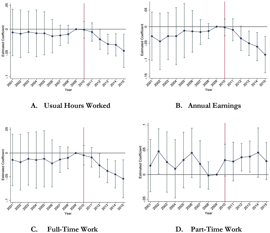
Notes: 95% confidence intervals adjusted for state-level clustering. Outcome is the log of the usual weekly hours worked per person in the last year (Panel A); log of total earnings in the last year (Panel B); log of the share with usual hours 35+; log of the share with usual hours 1-34. Outcomes are calculated using the ACS for the 16+ population. The 2004-2009 means for full-time work and part-time work are 54.3% and 15.7%, respectively.

The estimates reported in the figures are the coefficients on the pre-reformulation Non-Medical OxyContin Use rate interacted with calendar year indicators. The 2009 interaction is excluded and the corresponding estimate is normalized to 0. The estimated specification is represented by equation (1). The specification includes state and time fixed effects as well as time-varying controls: five age share variables, % white and non-Hispanic, % Hispanic, four education share variables, % foreign-born, and policy variables. Our policy variables are whether the state has a “must access” PDMP, pain clinic regulations, and legal and operational medical marijuana dispensaries. We also jointly estimate effects for pain reliever misuse interacted with year indicators.

Appendix Figure 6: Non-Medical OxyContin Use Event Study Estimates for Health Insurance.

Notes: 95% confidence intervals adjusted for state-level clustering. Outcome is the log of the share with any health insurance (Panel A); log of the share with employer-sponsored health insurance (Panel B). Outcomes are calculated using the ACS for the 16+ population. Health insurance information in the ACS is available beginning in 2008. N=408. The 2008-2009 means are 83.4% and 58.6% for health insurance and employer-sponsored health insurance, respectively.

The estimates reported in the figures are the coefficients on the pre-reformulation Non-Medical OxyContin Use rate interacted with calendar year indicators. The 2009 interaction is excluded and the corresponding estimate is normalized to 0. The estimated specification is represented by equation (1). The specification includes state and time fixed effects as well as time-varying controls: five age share variables, % white and non-Hispanic, % Hispanic, four education share variables, % foreign-born, and policy variables. Our policy variables are whether the state has a “must access” PDMP, pain clinic regulations, and legal and operational medical marijuana dispensaries. We also jointly estimate effects for pain reliever misuse interacted with year indicators.

Appendix Figure 7: Non-Medical OxyContin Use Average Effect Estimates by Demographics.

Source: American Community Survey

Notes: 95% confidence intervals adjusted for state-level clustering. Outcome is the log of the share of people working in the listed demographic. Estimates presented are average effects for the pre-reformulation OxyContin misuse variable using equation (2). Each estimate refers to a separate regression, which includes state and year fixed effects. We also control for the set of covariates listed in the notes of Figure 3. Regression is population-weighted. “HS Degree” represents the group with at most a high school degree (i.e., no college). “Some College” represents the group with at least some college education.

Appendix Figure 8: Non-Medical OxyContin Use Average Effect Estimates by Industry.

Source: Bureau of Economic Analysis industry data. We combined agriculture and forestry. We also combined all service industries into one category.

Notes: 95% confidence intervals, represented by the red lines, adjusted for state-level clustering. Outcome is the log of the number of jobs in the listed industry scaled by the 16+ population. The “Total Employment” estimate refers to the Table 2, Panel A, Column 1 estimate. Estimates presented are average effects for the pre-reformulation OxyContin misuse variable using equation (2). Each estimate refers to a separate regression, which includes state and year fixed effects. We also control for the set of covariates listed in the notes of Figure 3. Regression is population-weighted.

Appendix Figure 9: Non-Medical OxyContin Use Event Study Estimates for BEA Employment Rate and Percentage Applying for Disability Insurance, Robustness Tests.

Notes: 95% confidence intervals adjusted for state-level clustering. Outcome is the log of the employment-to-population ratio (Panels A, C) and the log of the percentage applying for disability insurance (Panels B, D). Outcomes are calculated using the BEA for ages 16+ and SSA Fiscal Year Disability Claim data set for ages 18-64.

The estimates reported in the figures are the coefficients on the pre-reformulation Non-Medical OxyContin Use rate interacted with calendar year indicators. The 2009 interaction is excluded and the corresponding estimate is normalized to 0. The estimated specification is represented by equation (1). The specification includes state and time fixed effects as well as covariates listed in notes for Figure 3. We also jointly estimate effects for pain reliever misuse interacted with year indicators. In Panels A and B, we add a Bartik prediction as described in the text. In Panels C and D, we add a Bartik prediction specific to manufacturing to permit manufacturing labor demand shocks to have independent effects on state labor/disability outcomes.

Appendix Tables

Appendix Table 1:

Average Effect Estimates for Log of Percentage of 18-64 Adults Receiving Disability Insurance for Listed Diagnostic Condition

Outcome:	% Ages 18-64 Receiving Disability Benefits by Condition
	Mental	Musculoskeletal	Nervous System	Neoplasms
OxyContin Misuse	0.02 (0.034)	0.068 (0.054)	0.055 (0.035)	0.024 (0.037)
Pain Reliever Misuse	0.009 (0.007)	0.016 (0.011)	0.008 (0.006)	0.004 (0.008)
Mean %	1.5%	1.0%	0.4%	0.1%

Notes:

^***1% significance,

^**5% significance,

^*10% significance.

All models include state and time fixed effects plus covariates mentioned in notes of Figure 5. Estimates presented are average effects for each pre-reformulation misuse variable using equation (2) and Figure 5. The outcome is logged. N=765. Standard errors are adjusted state-level clustering.

Appendix Table 2:

Average Effect Estimates for Percentage Working and Percentage Applying for Disability Insurance, Conditional on Census Division-Year Interactions

Panel A Outcome:	Percentage Working (BEA)
	(1)	(2)	(3)
OxyContin Misuse	−0.034** (0.015)	−0.040*** (0.015)	−2.199** (1.086)
Pain Reliever Misuse	0.007 (0.005)	0.009* (0.005)	0.414 (0.359)
OLS/Poisson Outcome	OLS Log	Poisson Total	OLS Level
Panel B Outcome:	% Apply for Disability
	(1)	(2)	(3)
OxyContin Misuse	0.189 (0.144)	0.287* (0.149)	0.209 (0.163)
Pain Reliever Misuse	−0.016 (0.039)	−0.049 (0.038)	−0.023 (0.044)
OLS/Poisson Outcome	OLS Log	Poisson Total	OLS Level

Notes:

^***1% significance,

^**5% significance,

^*10% significance.

All models include state and Census division-time fixed effects plus covariates mentioned in notes of Figure 5. Estimates presented are average effects for each pre-reformulation misuse variable using equation (2). When Poisson estimation is used, the outcome is the total and population is used as an exposure variable. N=765. Standard errors are adjusted state-level clustering.

References

- Abouk Rahi, Helmchen Lorens, Moghtaderi Ali, and Pines Jesse. “The ACA Medicaid Expansions and Opioid Mortality: Is There a Link?.” Medical Care Research and Review (2020): 1077558720967227. [DOI] [PubMed] [Google Scholar]
- Acemoglu Daron, Autor David, Dorn David, Hanson Gordon H., and Price Brendan. “Import competition and the great US employment sag of the 2000s.” Journal of Labor Economics 34, no. S1 (2016): S141–S198. [Google Scholar]
- Aliprantis Dionissi, Fee Kyle, and Schweitzer Mark E.. “Opioids and the Labor Market.” (2019). https://www.clevelandfed.org/en/newsroom-and-events/publications/working-papers/2019-working-papers/wp-1807r-opioids-and-labor-market.aspx
- Alpert Abby E., Evans William N., Lieber Ethan MJ, and Powell David. Origins of the Opioid Crisis and Its Enduring Imfacts. No. w26500. National Bureau of Economic Research, 2019. [DOI] [PMC free article] [PubMed] [Google Scholar]
- Alpert Abby, Powell David, and Pacula Rosalie Liccardo. “Supply-side drug policy in the presence of substitutes: Evidence from the introduction of abuse-deterrent opioids.” American Economic Journal: Economic Policy 10, no. 4 (2018): 1–35. [DOI] [PMC free article] [PubMed] [Google Scholar]
- Autor David H., and Duggan Mark G.. “The rise in the disability rolls and the decline in unemployment.” The Quarterly Journal of Economics 118, no. 1 (2003): 157–206. [Google Scholar]
- Autor David H., Dom David, and Hanson Gordon H.. “The China syndrome: Local labor market effects of import competition in the United States.” American Economic Review 103, no. 6 (2013): 2121–68. [Google Scholar]
- Autor David H., Maestas Nicole, Mullen Kathleen J., and Strand Alexander. Does delay cause decay? The effect of administrative decision time on the labor force participation and earnings of disability applicants. No. w20840. National Bureau of Economic Research, 2015. [Google Scholar]
- Bartholow Michael. “Top 200 drugs of 2010.” Pharmacy Times 77, no. 5 (2011): 52. [Google Scholar]
- Bartik Timothy J. “Who benefits from state and local economic development policies?” W.E. Upjohn Institute for Employment Research (1991). [Google Scholar]
- Becker William C., and Fiellin David A.. “Abuse-deterrent opioid formulations–putting the potential benefits into perspective.” New England Journal of Medicine 376, no. 22 (2017): 2103–2105. [DOI] [PubMed] [Google Scholar]
- Beheshti David. “Adverse health effects of abuse-deterrent opioids: Evidence from the reformulation of OxyContin.” Health Economics 28, no. 12 (2019): 1449–1461. [DOI] [PubMed] [Google Scholar]
- Beheshti David. “The Impact of Opioids on the Labor Market: Evidence from Drug Rescheduling.” Working Paper (2019). [Google Scholar]
- Betz Michael R., and Jones Lauren E.. “Wage and employment growth in America’s drug epidemic: Is all growth created equal?” American Journal of Agricultural Economics 100, no. 5 (2018): 1357–1374. [DOI] [PMC free article] [PubMed] [Google Scholar]
- Black Dan, Daniel Kermit, and Sanders Seth. “The impact of economic conditions on participation in disability programs: Evidence from the coal boom and bust.” American Economic Review 92, no. 1 (2002): 27–50. [DOI] [PubMed] [Google Scholar]
- Blanchard Olivier and Katz Lawrence F.. “Regional evolutions.” Brookings Papers on Economic Activity, Economic Studies Program, The Brookings Institution; 23, no. 1 (1992). [Google Scholar]
- Brucker Debra. “Estimating the prevalence of substance use, abuse, and dependence among Social Security Disability benefit recipients.” Journal of Disability Policy Studies 18, no. 3 (2007): 148–159. [Google Scholar]
- Bütikofer Aline, and Skira Meghan M.. “Missing Work Is a Pain The Effect of Cox-2 Inhibitors on Sickness Absence and Disability Pension Receipt.” Journal of Human Resources 53, no. 1 (2018): 71–122. [Google Scholar]
- Caulkins Jonathan P., Kilmer Beau, Reuter Peter H., and Midgette Greg. “Cocaine’s fall and marijuana’s rise: questions and insights based on new estimates of consumption and expenditures in US drug markets.” Addiction 110, no. 5 (2015): 728–736. [DOI] [PubMed] [Google Scholar]
- Charles Kerwin Kofi, Hurst Erik, and Schwartz Mariel. “The transformation of manufacturing and the decline in US employment.” NBER Macroeconomics Annual 33, no. 1 (2019): 307–372. [Google Scholar]
- Charles Kerwin Kofi, Li Timing, and Stephens Melvin Jr. “Disability benefit take-up and local labor market conditions.” Review of Economics and Statistics 100, no. 3 (2018): 416–423. [Google Scholar]
- Ciani Emanuele, and Fisher Paul. “Dif-in-dif estimators of multiplicative treatment effects.” Journal of Econometric Methods 8, no. 1 (2018). [Google Scholar]
- Cicero Theodore J., and Ellis Matthew S.. “Abuse-deterrent formulations and the prescription opioid abuse epidemic in the United States: lessons learned from OxyContin.” JATMA Psychiatry 72, no. 5 (2015): 424–430. [DOI] [PubMed] [Google Scholar]
- Cicero Theodore J., Inciardi James A., and Munoz Alvaro. “Trends in abuse of OxyContin® and other opioid analgesics in the United States: 2002–2004.” The Journal of Pain 6, no. 10 (2005): 662–672. [DOI] [PubMed] [Google Scholar]
- Currie Janet, Jin Jonas, and Schnell Molly. “US Employment and Opioids: Is There a Connection?” In Health and Labor Markets, pp. 253–280. Emerald Publishing Limited, 2019. [Google Scholar]
- Davis Matthew A., Lin Lewei A., Liu Haiyin, and Sites Brian D.. “Prescription opioid use among adults with mental health disorders in the United States.” The Journal of the American Board of Family Medicine 30, no. 4 (2017): 407–417. [DOI] [PubMed] [Google Scholar]
- Deiana Claudio, and Giua Ludovica. “The US Opioid Epidemic: Prescription Opioids, Labour Market Conditions and Crime.” Working Paper (2019). [Google Scholar]
- DeSimone Jeff. “Illegal drug use and employment.” Journal of Labor Economics 20, no. 4 (2002): 952–977. [Google Scholar]
- Evans Mary F., Harris Matthew, and Kessler Lawrence. “The Hazards of Unwinding the Prescription Opioid Epidemic: Implications for Child Abuse and Neglect.” Available at SSRN 3582060 (2020). [Google Scholar]
- Evans William N., Lieber Ethan MJ, and Power Patrick. “How the reformulation of OxyContin ignited the heroin epidemic.” Review of Economics and Statistics 101, no. 1 (2019): 1–15. [Google Scholar]
- Feingold Daniel, Brill Silviu, Goor-Aryeh Itay, Delayahu Yael, and Lev-Ran Shaul. “The association between severity of depression and prescription opioid misuse among chronic pain patients with and without anxiety: a cross-sectional study.” Journal of Affective Disorders 235 (2018): 293–302. [DOI] [PubMed] [Google Scholar]
- Finsterer Josef, and Stollberger Claudia. “Neurological Abnormalities in Opiate Addicts.” In Neuropathology of Drug Addictions and Substance Misuse, pp. 947–955. Academic Press, 2016. [Google Scholar]
- Franco Armando, Wagner Zachary, and Whaley Christopher M.. “Doped up or Dropped Out: The Effects of Opioid Use on Workplace Absences.” Working Paper (2019). [Google Scholar]
- French Michael T., Christopher Roebuck M, and Kebreau Alexandre Pierre. “Illicit drug use, employment, and labor force participation.” Southern Economic Journal (2001): 349–368. [Google Scholar]
- French Eric, and Song Jae. “The effect of disability insurance receipt on labor supply.” American Economic Journal: Economic Policy 6, no. 2 (2014): 291–337. [Google Scholar]
- Garthwaite Craig L. “The economic benefits of pharmaceutical innovations: The case of Cox-2 inhibitors.” American Economic Journal: Applied Economics 4, no. 3 (2012): 116–37. [Google Scholar]
- Ghimire Keshar M., and Catherine Maclean Johanna. “Medical marijuana and workers’ compensation claiming.” Health Economics (2020). [DOI] [PubMed] [Google Scholar]
- Gittell Ross, Samuels Jon D., and Tebaldi Edinaldo. “The Contribution of Associate’s Degree Holders to US Earnings, Labor Quality, Productivity, and Overall Economic Growth.” Southern Economic Journal 84, no. 2 (2017): 600–636. [Google Scholar]
- Gresenz Carole Roan, Watkins Katherine, and Podus Deborah. “Supplemental security income (SSI), disability insurance (DI), and substance abusers.” Community MentalHealth Journal 34, no. 4 (1998): 337–350. [DOI] [PubMed] [Google Scholar]
- Harris Matthew C., Kessler Lawrence M., Murray Matthew N., and Glenn Beth. “Prescription Opioids and Labor Market Pains: The Effect of Schedule II Opioids on Labor Force Participation and Unemployment.” Journal of ELuman Resources (2019): 1017–9093R2. [Google Scholar]
- IQVIA Institute. “Prescription Opioid Trends in the United States” (2020). https//:www.iqvia.com/insights/the-iqvia-institute/reports/prescription-opioid-trends-in-the-united-states (last accessed December 29, 2020).
- Jacobson Mireille. “Baby booms and drug busts: Trends in youth drug use in the United States, 1975–2000.” The Quarterly Journal of Economics 119, no. 4 (2004): 1481–1512. [Google Scholar]
- Jiang Ruixuan, Lee Inyoung, Lee Todd A., and Simon Pickard A. “The societal cost of heroin use disorder in the United States.” PloS one 12, no. 5 (2017): e0177323. [DOI] [PMC free article] [PubMed] [Google Scholar]
- Kaestner Robert. “The Effect of Illicit Drug Use on the Labor Supply of Young Adults.” Journal of Human Resources (1994): 126–155. [Google Scholar]
- Kaestner Robert, and Ziedan Engy. Mortality and socioeconomic consequences of prescription opioids: Evidence from state policies. No. w26135. National Bureau of Economic Research, 2020. [Google Scholar]
- Kahn-Lang Ariella, and Lang Kevin. “The Promise and Pitfalls of Differences-in-Differences: Reflections on 16 and Pregnant and Other Applications.” Journal of Business zrt Economic Statistics (2019): 1–14. [Google Scholar]
- Kilby Angela. “Opioids for the masses: welfare tradeoffs in the regulation of narcotic pain medications.” Cambridge: Massachusetts Institute of Technology (2015). [Google Scholar]
- Kolodny Andrew, Courtwright David T., Hwang Catherine S., Kreiner Peter, Eadie John L., Clark Thomas W., and Caleb Alexander G. “The prescription opioid and heroin crisis: a public health approach to an epidemic of addiction.” Annual Review of Public Health 36 (2015): 559–574. [DOI] [PubMed] [Google Scholar]
- Krueger Alan B. “Where have all the workers gone? An inquiry into the decline of the US labor force participation rate.” Brookings Papers on Economic Actirity 2017, no. 2 (2017): 1. [DOI] [PMC free article] [PubMed] [Google Scholar]
- Liebman Jeffrey B. “Understanding the increase in disability insurance benefit receipt in the United States.” Journal of Economic Perspectives 29, no. 2 (2015): 123–50. [DOI] [PubMed] [Google Scholar]
- MacDonald Ziggy, and Pudney Stephen. “Illicit drug use, unemployment, and occupational attainment.” Journal of Elealth Economics 19, no. 6 (2000): 1089–1115. [DOI] [PubMed] [Google Scholar]
- Maclean Johanna Catherine, Ghimire Keshar M., and Hersch Nicholas Lauren. “Medical marijuana laws and disability applications, receipts, and terminations.” National Bureau of Economic Research Working Paper No. 23862 (2019). [Google Scholar]
- Maclean Catherine, Mallatt Justine, Ruhm Christopher J., and Simon Kosali. “Review of Economic Studies on the Opioid Crisis.” NBER Working Paperw28067 (2020). [Google Scholar]
- Maestas Nicole, Mullen Kathleen J., and Powell David. The effect of population aging on economic growth, the labor force and productivity. No. w22452. National Bureau of Economic Research, 2016. [Google Scholar]
- Maestas Nicole, Mullen Kathleen J., and Strand Alexander. “Does disability insurance receipt discourage work? Using examiner assignment to estimate causal effects of SSDI receipt.” American Economic Review 103, no. 5 (2013): 1797–1829. [Google Scholar]
- Maestas Nicole, Mullen Kathleen J., and Strand Alexander. The effect of economic conditions on the disability insurance program: Evidence from the GreatRecession. No. w25338. National Bureau of Economic Research, 2018. [Google Scholar]
- Mallatt Justine. “Policy-induced substitution to illicit drugs and implications for law enforcement activity.” SSRN Scholarly Paper ID 3418615. Social Science Research Network, Rochester, NY: (2020). [Google Scholar]
- McCully Clinton P. “Integration of Micro-and Macrodata on Consumer Income and Expenditures.” In Measuring Economic Sustainability and Progress, pp. 137–179. University of Chicago Press, 2014. [Google Scholar]
- Moore Timothy J. “The employment effects of terminating disability benefits.” Journal of Public Economics 124 (2015): 30–43. [Google Scholar]
- Nicholas Lauren Hersch, and Maclean Johanna Catherine. “The effect of medical marijuana laws on the health and labor supply of older adults: Evidence from the Health and Retirement Study.” Journal of Policy Analysis and Management 38, no. 2 (2019): 455–480. [PubMed] [Google Scholar]
- Pardo Bryce, Caulkins Jonathan P., Kilmer Beau, Pacula Rosalie Liccardo, Reuter Peter, and Stein Bradley D.. “The Synthetic Opioid Surge in the United States” (2019). https://www.rand.org/pubs/research_reports/RR3116.html [Google Scholar]
- Powell David, Alpert Abby, and Pacula Rosalie L.. “A Transitioning Epidemic: How The Opioid Crisis Is Driving The Rise In Hepatitis C.” Health Affairs 38, no. 2 (2019): 287–294. [DOI] [PubMed] [Google Scholar]
- Powell David, Pacul Rosalie Liccardo, and Jacobson Mireille. “Do medical marijuana laws reduce addictions and deaths related to pain killers?” Journal of Health Economics 58 (2018): 29–42. [DOI] [PMC free article] [PubMed] [Google Scholar]
- Powell David and Pacula Rosalie Liccardo. “The evolving consequences of OxyContin reformulation on drug overdoses.” American Journal of Health Economics, 2021. [DOI] [PMC free article] [PubMed] [Google Scholar]
- Sabia Joseph J., and Nguyen Thanh Tam. “The effect of medical marijuana laws on labor market outcomes.” The Journal of Law and Economics 61, no. 3 (2018): 361–396. [Google Scholar]
- Santos Silva JMC, and Tenreyro Silvana. “The log of gravity.” The Review of Economics and Statistics 88, no. 4 (2006): 641–658. [Google Scholar]
- Savych Bogdan, Neumark David, and Lea Randall. “Do opioids help injured workers recover and get back to work? The impact of opioid prescriptions on duration of temporary disability.” Industrial Relations: A Journal of Economy and Society 58, no. 4 (2019): 549–590. [Google Scholar]
- Scholl Lawrence, Seth Puja, Kariisa Mbabazi, Wilson Nana, and Baldwin Grant. “Drug and opioid-involved overdose deaths–United States, 2013–2017.” Morbidity and Mortality Weekly Report 67, no. 5152 (2019): 1419. [DOI] [PMC free article] [PubMed] [Google Scholar]
- Substance Abuse and Mental Health Services Administration (SAMHSA). “2018 National Survey on Drug Use and Health Methodological Resource Book” (2019). https://www.samhsa.gov/data/sites/default/files/cbhsq-reports/NSDUHmrbSampleDesign2018/NSDUHmrbSampleDesign2018.pdf
- Williams Jenny, Pacula Rosalie Liccardo, and Smart Rosanna. De Facto or De Jure? Ethnic Differences in Quit Responses to Legal Protections of Medical Marijuana Dispensaries. No. w25555. National Bureau of Economic Research, 2019. [Google Scholar]
- Zarkin Gary A., Mroz Thomas A., Bray Jeremy W., and French Michael T.. “The relationship between drug use and labor supply for young men.” Labour Economics 5, no. 4 (1998): 385–409. [Google Scholar]