Randomized Linear Algebra Approaches to Estimate the Von Neumann Entropy of Density Matrices

Abstract

The von Neumann entropy, named after John von Neumann, is an extension of the classical concept of entropy to the field of quantum mechanics. From a numerical perspective, von Neumann entropy can be computed simply by computing all eigenvalues of a density matrix, an operation that could be prohibitively expensive for large-scale density matrices. We present and analyze three randomized algorithms to approximate von Neumann entropy of real density matrices: our algorithms leverage recent developments in the Randomized Numerical Linear Algebra (RandNLA) literature, such as randomized trace estimators, provable bounds for the power method, and the use of random projections to approximate the eigenvalues of a matrix. All three algorithms come with provable accuracy guarantees and our experimental evaluations support our theoretical findings showing considerable speedup with small loss in accuracy.

I. Introduction

Entropy is a fundamental quantity in many areas of science and engineering. von Neumann entropy, named after John von Neumann, is an extension of classical entropy concepts to the field of quantum mechanics. Its foundations can be traced to von Neumann’s work on Mathematische Grundlagen der Quantenmechanik¹. In his work, Von Neumann introduced the notion of a density matrix, which facilitated extension of the tools of classical statistical mechanics to the quantum domain in order to develop a theory of quantum mechanics.

From a mathematical perspective (see Section I-A for details) the real density matrix R is a symmetric positive semidefinite matrix in ${\mathbb{R}}^{n\times n}$ with unit trace. Let p_i, i = 1 … n be the eigenvalues of R in decreasing order; then, the entropy of R is defined as²

$$\mathcal{H}(\mathbf{R})=-\sum _{i=1}^n{p}_i\text{ln}{p}_i.$$ (1)

The above definition is a proper extension of both the Gibbs entropy and the Shannon entropy to the quantum case. It implies an obvious algorithm to compute $\mathcal{H}(\mathbf{R})$ by computing the eigendecomposition of R; known algorithms for this task can be prohibitively expensive for large values of n, particularly when the matrix becomes dense [1]. For example, [2] describes an entangled two-photon state generated by spontaneous parametric down-conversion, which can result in a sparse and banded density matrix with n ≈ 10⁸.

Motivated by the high computational cost, we seek numerical algorithms that approximate the von Neumann entropy of large density matrices, e.g., symmetric positive definite matrices with unit trace, faster than the trivial $\mathcal{O}(n^3)$ approach. Our algorithms build upon recent developments in the field of Randomized Numerical Linear Algebra (RandNLA), an interdisciplinary research area that exploits randomization as a computational resource to develop improved algorithms for large-scale linear algebra problems. Indeed, our work here focuses at the intersection of RandNLA and information theory, delivering novel randomized linear algebra algorithms and related quality-of-approximation results for a fundamental information-theoretic metric.

A. Background

We focus on finite-dimensional function (state) spaces. In this setting, the density matrix R represents the statistical mixture of k ≤ n pure states, and has the form

$$\text{R}=\sum _{i=1}^k{p}_i{\mathit{\psi }}_i{\mathit{\psi }}_i^T\in {\mathbb{R}}^{n\times n}.$$ (2)

The vectors ${\mathit{\psi }}_i\in {\mathbb{R}}^n$ for i = 1 … k represent the k ≤ n pure states and can be assumed to be pairwise orthogonal and normal, while p_i’s correspond to the probability of each state and satisfy p_i > 0 and ${\sum }_{i=1}^k{p}_i=1$. From a linear algebraic perspective, eqn. (2) can be rewritten as

$$\mathbf{R}=\mathbf{\Psi }{\mathbf{\Sigma }}_p{\mathbf{\Psi }}^T\in {\mathbb{R}}^{n\times n},$$ (3)

where $\mathbf{\Psi }\in {\mathbb{R}}^{n\times k}$ is the matrix whose columns are the vectors ψ_i and ${\mathbf{\Sigma }}_p\in {\mathbb{R}}^{k\times k}$ is a diagonal matrix whose entries are the (positive) p_i’s. Given our assumptions for ψ_i, Ψ^TΨ = I; also R is symmetric positive semidefinite with its eigenvalues equal to p_i and corresponding left/right singular vectors equal to ψ_i’s; and $\mathbf{tr}(\mathbf{R})={\sum }_{i=1}^k{p}_i=1$. Notice that eqn. (3) essentially reveals the (thin) Singular Value Decomposition (SVD) [1] of R. The Von Neumann entropy of R, denoted by $\mathcal{H}(\mathbf{R})$ is equal to (see also eqn. (1))

$$\mathcal{H}\left(\mathbf{R}\right)=\sum _{i:p_i>0}{p}_i\text{ln}{p}_i=-\mathbf{tr}\left(\mathbf{R}\text{ln}\mathbf{R}\right).$$ (4)

The second equality follows from the definition of matrix functions [3]. More precisely, we overload notation and consider the full SVD of R, namely R = ΨΣ_pΨ^T, where $\mathbf{\Psi }\in {\mathbb{R}}^{n\times n}$ is an orthogonal matrix whose top k columns correspond to the k pure states and the bottom n − k columns are chosen so that ΨΨ^T = Ψ^TΨ = I_n. Here Σ_p is a diagonal matrix whose bottom n−k diagonal entries are set to zero. Let h(x) = x ln x for any x > 0 and let h(0) = 0. Then, using the cyclical property of the trace and the definition of h(x),

$$\begin{gathered} -\sum _{i,p_i>0}{p}_i\text{ln}{p}_i=-\mathbf{tr}\left(\mathbf{\Psi }h\left({\mathbf{\Sigma }}_p\right){\mathbf{\Psi }}^T\right) \\ =-\mathbf{tr}\left(h\left(\mathbf{R}\right)\right) \\ =-\mathbf{tr}\left(\mathbf{R}\text{ln}\mathbf{R}\right). \end{gathered}$$ (5)

B. Trace estimators

The following lemma appeared in [4] and is immediate from Theorem 5.2 in [5]. It implies an algorithm to approximate the trace of any symmetric positive semidefinite matrix A by computing inner products of the matrix with Gaussian random vectors.

Lemma 1. Let $\mathbf{A}\in {\mathbb{R}}^{n\times n}$ be a positive semi-definite matrix, let 0 < ϵ < 1 be an accuracy parameter, and let 0 < δ < 1 be a failure probability. If ${\mathbf{g}}_1,{\mathbf{g}}_2,\dots ,{\mathbf{g}}_s\in {\mathbb{R}}^n$ are independent random standard Gaussian vectors, then, for s = ⌈20 ln(2/δ)/ϵ²⌉, with probability at least 1 − δ,

$$\left|\mathbf{tr}\left(\mathbf{A}\right)-\frac{1}{s}\sum _{i=1}^s{\mathbf{g}}_i^{{\rm T}}{\mathbf{Ag}}_i\right|\le \in ·\mathbf{tr}\left(\mathbf{A}\right).$$

C. Our contributions

We present and analyze three randomized algorithms to approximate the von Neumann entropy of density matrices. The first two algorithms (Sections II and III) leverage two different polynomial approximations of the matrix function $\mathcal{H}(\mathbf{R})=-\mathbf{tr}(\mathbf{R}\ln \mathbf{R})$: the first approximation uses a Taylor series expansion, while the second approximation uses Chebyschev polynomials. Both algorithms return, with high probability, relative-error approximations to the true entropy of the input density matrix, under certain assumptions. More specifically, in both cases, we need to assume that the input density matrix has n non-zero eigenvalues, or, equivalently, that the probabilities p_i, i = 1 … n, corresponding to the underlying n pure states are non-zero. The running time of both algorithms is proportional to the sparsity of the input density matrix and depends (see Theorems 2 and 4 for precise statements) on, roughly, the ratio of the largest to the smallest probability p₁/p_n (recall that the smallest probability is assumed to be non-zero), as well as the desired accuracy.

The third algorithm (Section V) is fundamentally different, if not orthogonal, to the previous two approaches. It leverages the power of random projections [6], [7] to approximate numerical linear algebra quantities, such as the eigenvalues of a matrix. Assuming that the density matrix R has exactly k ⪡ n non-zero eigenvalues, e.g., there are k pure states with non-zero probabilities p_i, i = 1 … k, the proposed algorithm returns, with high probability, relative error approximations to all k probabilities p_i. This, in turn, implies an additive-relative error approximation to the entropy of the density matrix, which, under a mild assumption on the true entropy of the density matrix, becomes a relative error approximation (see Theorem 10 for a precise statement). The running time of the algorithm is again proportional to the sparsity of the density matrix and depends on the target accuracy, but, unlike the previous two algorithms, does not depend on any function of the p_i.

From a technical perspective, the theoretical analysis of the first two algorithms proceeds by combining the power of polynomial approximations, either using Taylor series or Chebyschev polynomials, to matrix functions, combined with randomized trace estimators. A provably accurate variant of the power method is used to estimate the largest probability p_i. If this estimate is significantly smaller than one, it can improve the running times of the proposed algorithms (see discussion after Theorem 2). The third algorithm leverages a powerful, multiplicative matrix perturbation result that first appeared in [8]. Our work in Section V is a novel application of this inequality to derive bounds for RandNLA algorithms.

Finally, in Section VI, we present a detailed evaluation of our algorithms on synthetic density matrices of various sizes, most of which were generated using Matlab’s QETLAB toolbox [9]. For some of the larger matrices that were used in our evaluations, the exact computation of the entropy takes hours, whereas our algorithms return approximations with relative errors well below 0.5% in only a few minutes.

D. Prior work

The first non-trivial algorithm to approximate the von Neumann entropy of a density matrix appeared in [2]. Their approach is essentially the same as our approach in Section III. Indeed, our algorithm in Section III was inspired by their approach. However, our analysis is somewhat different, lever-aging a provably accurate variant of the power method, as well as provably accurate trace estimators to derive a relative error approximation to the entropy of a density matrix, under appropriate assumptions. A detailed, technical comparison between our results in Section III and the work of [2] is delegated to Section III-C.

Independently and in parallel with our work, [10] presented a multipoint interpolation algorithm (building upon [11]) to compute a relative error approximation for the entropy of a real matrix with bounded condition number. The proposed running time of Theorem 35 of [10] does not depend on the condition number of the input matrix (i.e., the ratio of the largest to the smallest probability), which is a clear advantage in the case of ill-conditioned matrices. However, the dependence of the algorithm of Theorem 35 of [10] on terms like (log n/ϵ)⁶ or $n^{1/3}\text{nnz}(\mathbf{A})+n\sqrt{\text{nnz}(\mathbf{A})}$ (where nnz(A) represents the number of non-zero elements of the matrix A) could blow up the running time of the proposed algorithm for reasonably conditioned matrices.

We also note the recent work in [4], which used Taylor approximations to matrix functions to estimate the log determinant of symmetric positive definite matrices (see also Section 1.2 of [4] for an overview of prior work on approximating matrix functions via Taylor series). The work of [12] used a Chebyschev polynomial approximation to estimate the log determinant of a matrix and is reminiscent of our approach in Section III and, of course, the work of [2].

We conclude this section by noting that our algorithms use two tools (described, for the sake of completeness, in the Appendix) that appeared in prior work. The first tool is the power method, with a provable analysis that first appeared in [13]. The second tool is a provably accurate trace estimation algorithm for symmetric positive semidefinite matrices that appeared in [5].

II. An approach via Taylor series

Our first approach to approximate the von Neumann entropy of a density matrix uses a Taylor series expansion to approximate the logarithm of a matrix, combined with a relative-error trace estimator for symmetric positive semi-definite matrices and the power method to upper bound the largest singular value of a matrix.

A. Algorithm and Main Theorem

Our main result is an analysis of Algorithm 1 (see below) that guarantees relative error approximation to the entropy of the density matrix R, under the assumption that $\mathbf{R}={\sum }_{i=1}^n{p}_i{\mathit{\psi }}_i{\mathit{\psi }}_i^T\in {\mathbb{R}}^{n\times n}$ has n pure states with 0 < ℓ ≤ p_i for all i = 1 … n. The following theorem is our main quality-of-approximation result for Algorithm 1.

Algorithm 1.

A Taylor series approach to estimate the entropy.

1:	INPUT: $\mathbf{R}\in {\mathbb{R}}^{n\times n}$, accuracy parameter ε > 0, failure probability δ, and integer m > 0.
2:	Compute ${\tilde{p}}_1$, the estimate of the largest eigenvalue of R, p1, using Algorithm 8 (see Appendix) with $t=\mathcal{O}(\ln n)$ and $q=\mathcal{O}(\ln (1/\delta ))$.
3:	Set $u=\min \{1,6{\tilde{p}}_1\}$.
4:	Set s = ⌈20 ln(2/δ)/ε2⌉.
5:	Let ${\mathbf{g}}_1,{\mathbf{g}}_2,\dots ,{\mathbf{g}}_s\in {\mathbb{R}}^n$ be i.i.d. random Gaussian vectors.
6:	OUTPUT: return $\widehat{\mathcal{H}}\left(\mathbf{R}\right)=\text{ln}{u}^{-1}+\frac{1}{s}\sum _{i=1}^s\sum _{k=1}^m\frac{{\mathbf{g}}_i^T\mathbf{R}{\left({\mathbf{I}}_n-u^{-1}\mathbf{R}\right)}^k{\mathbf{g}}_i}{k}$.

Theorem 2. Let R be a density matrix such that all probabilities p_i, i = 1 … n satisfy 0 < ℓ ≤ p_i. Let u be computed as in Algorithm 1 and let $\widehat{\mathcal{H}}(\mathbf{R})$ be the output of Algorithm 1 on inputs R, m, and ϵ < 1; Then, with probability at least 1 − 2δ,

$$\left|\widehat{\mathcal{H}}\left(\mathbf{R}\right)-\mathcal{H}\left(\mathbf{R}\right)\right|\le 2ϵ\mathcal{H}\left(\mathbf{R}\right),$$

by setting $m=\lceil \frac{u}{\ell }\text{ln}\frac{1}{ϵ}\rceil$. The algorithm runs in time

$$\mathcal{O}\left(\left(\frac{u}{\ell }·\frac{\text{ln}\left(1/ϵ\right)}{{ϵ}^2}+\text{ln}\left(n\right)\right)\text{ln}\left(1/\delta \right)·\text{nnz}\left(\mathbf{R}\right)\right).$$

A few remarks are necessary to better understand the above theorem. First, ℓ could be set to p_n, the smallest of the probabilities corresponding to the n pure states of the density matrix R. Second, it should be obvious that u in Algorithm 1 could be simply set to one and thus we could avoid calling Algorithm 8 to estimate p₁ by ${\tilde{p}}_1$ and thus compute u. However, if p₁ is small, then u could be significantly smaller than one, thus reducing the running time of Algorithm 1, which depends on the ratio u/l. Third, ideally, if both p₁ and p_n were used instead of u and l, respectively, the running time of the algorithm would scale with the ratio p₁/p_n.

B. Proof of Theorem 2

We now prove Theorem 2, which analyzes the performance of Algorithm 1. Our first lemma presents a simple expression for $\mathcal{H}(\mathbf{R})$ using a Taylor series expansion.

Lemma 3. Let $\mathbf{R}\in {\mathbb{R}}^{n\times n}$ be a symmetric positive definite matrix with unit trace and whose eigenvalues lie in the interval [ℓ, u], for some 0 < ℓ ≤ u ≤ 1. Then,

$$\mathcal{H}\left(\mathbf{R}\right)=\text{ln}{u}^{-1}+\sum _{k=1}^{\infty }\frac{\mathbf{tr}\left(\mathbf{R}{\left({\mathbf{I}}_n-u^{-1}\mathbf{R}\right)}^k\right)}{k}.$$

Proof: From the definition of the von Neumann entropy and a Taylor expansion,

$$\begin{gathered} \mathcal{H}\left(\mathbf{R}\right)=-\mathbf{tr}\left(\mathbf{R}\text{ln}\left(u{u}^{-1}\mathbf{R}\right)\right) \\ =-\mathbf{tr}\left(\left(\text{ln}\text{u}\right)\mathbf{R}\right)-\mathbf{tr}\left(\mathbf{R}\text{ln}\left({\mathbf{I}}_n-\left({\mathbf{I}}_n-u^{-1}\mathbf{R}\right)\right)\right) \\ =\text{ln}{u}^{-1}-\mathbf{tr}\left(-\mathbf{R}\sum _{k=1}^{\infty }\frac{{\left({\mathbf{I}}_n-u^{-1}\mathbf{R}\right)}^k}{k}\right) \\ =\text{ln}{u}^{-1}+\sum _{k=1}^{\infty }\frac{\mathbf{tr}\left(\mathbf{R}{\left({\mathbf{I}}_n-u^{-1}\mathbf{R}\right)}^k\right)}{k}. \end{gathered}$$ (6)

Eqn. (6) follows since R has unit trace and from a Taylor expansion: indeed, $\text{ln}({\mathbf{I}}_n-\mathbf{A})=-{\sum }_{k=1}^{\infty }{\mathbf{A}}^k/k$ for a symmetric matrix A whose eigenvalues are all in the interval (−1, 1). We note that the eigenvalues of I_n − u⁻¹R are in the interval [0, 1 − (ℓ/u)], whose upper bound is strictly less than one since, by our assumptions, ℓ/u > 0.

We now proceed to prove Theorem 2. We will condition our analysis on Algorithm 8 being successful, which happens with probability at least 1 − δ. In this case, $u=\text{min}\{1,6{\tilde{p}}_1\}$ is an upper bound for all probabilities p_i. For notational convenience, set C = I_n − u⁻¹R. We start by manipulating $\Delta =|\widehat{\mathcal{H}}(\mathbf{R})-\mathcal{H}(\mathbf{R})|$ as follows:

$$\begin{gathered} \Delta =\left|\sum _{k=1}^m\frac{1}{k}·\frac{1}{s}\sum _{i=1}^s{\mathbf{g}}_i^{\text{T}}{\mathbf{RC}}^k{\mathbf{g}}_i-\sum _{k=1}^{\infty }\frac{1}{k}\mathbf{tr}\left({\mathbf{RC}}^k\right)\right| \\ \le \left|\sum _{k=1}^m\frac{1}{k}·\frac{1}{s}\sum _{i=1}^s{\mathbf{g}}_i^{\text{T}}{\mathbf{RC}}^k{\mathbf{g}}_i-\sum _{k=1}^{\infty }\frac{1}{k}\mathbf{tr}\left({\mathbf{RC}}^k\right)\right|+\left|\sum _{k=m+1}^{\infty }\frac{1}{k}\mathbf{tr}\left({\mathbf{RC}}^k\right)\right| \\ =\underset{{\Delta }_1}{\underbrace{\left|\frac{1}{s}\sum _{i=1}^s{\mathbf{g}}_i^{\text{T}}\left(\sum _{k=1}^m{\mathbf{RC}}^k/k\right){\mathbf{g}}_i-\mathbf{tr}\left(\sum _{k=1}^m{\mathbf{RC}}^k\right)\right|}}+\underset{{\Delta }_2}{\underbrace{\left|\sum _{k=m+1}^m\mathbf{tr}\left({\mathbf{RC}}^k\right)/k\right|}}. \end{gathered}$$

We now bound the two terms Δ₁ and Δ₂ separately. We start with Δ₁: the idea is to apply Lemma 1 on the matrix ${\sum }_{k=1}^m{\mathbf{RC}}_k/k$ with s = ⌈20 ln(2/δ)/ϵ²⌉. Hence, with probability at least 1 − δ:

$${\Delta }_1\le ϵ·\mathbf{tr}\left(\sum _{k=1}^m{\mathbf{RC}}^k/k\right)\le ϵ·\mathbf{tr}\left(\sum _{k=1}^{\infty }{\mathrm{RC}}^k/k\right).$$ (7)

A subtle point in applying Lemma 1 is that the matrix ${\sum }_{k=1}^m{\mathbf{RC}}^k/k$ must be symmetric positive semidefinite. To prove this, let the SVD of R be R = ΨΣ_pΨ^T, where all three matrices are in ${\mathbb{R}}^{n\times n}$ and the diagonal entries of Σ_p are in the interval [ℓ, u]. Then, it is easy to see that C = I_n − u⁻¹R = Ψ(I_n − u⁻¹Σ_p)Ψ^T and RC^k = ΨΣ_p(I_n − u⁻¹Σ_p)^kΨ^T, where the diagonal entries of I_n − u⁻¹Σ_p are non-negative, since the largest entry in Σ_p is upper bounded by u. This proves that RC^k is symmetric positive semidefinite for any k, a fact which will be useful throughout the proof. Now,

$$\sum _{k=1}^m{\mathbf{RC}}^k/k=\Psi \left({\mathbf{\Sigma }}_p\sum _{k=1}^m{\left({\mathbf{I}}_n-u^{-1}{\mathbf{\Sigma }}_p\right)}^k/k\right){\mathbf{\Psi }}^T,$$

which shows that the matrix of interest is symmetric positive semidefinite. Additionally, since RC^k is symmetric positive semidefinite, its trace is non-negative, which proves the second inequality in eqn. (7) as well.

We proceed to bound Δ₂ as follows:

$$\begin{gathered} {\Delta }_2=\left|\sum _{k=m+1}^{\infty }\mathbf{tr}\left({\mathbf{RC}}^k\right)/k\right| \\ =\left|\sum _{k=m+1}^{\infty }\mathbf{tr}\left({\mathbf{RC}}^m{\mathbf{C}}^{k-m}\right)/k\right| \\ =\left|\sum _{k=m+1}^{\infty }\mathbf{tr}\left({\mathbf{C}}^m{\mathbf{C}}^{k-m}\mathbf{R}\right)/k\right| \\ \le \left|\sum _{k=m+1}^{\infty }{\Vert {\mathbf{C}}^m\Vert }_2·\mathbf{tr}\left({\mathbf{C}}^{k-m}\mathbf{R}\right)/k\right| \end{gathered}$$ (8)

$$\begin{gathered} ={\Vert {\mathbf{C}}^m\Vert }_2·\left|\sum _{k=m+1}^{\infty }\mathbf{tr}\left({\mathbf{RC}}^{k-m}\right)/k\right| \\ \le {\Vert {\mathbf{C}}^m\Vert }_2·\left|\sum _{k=1}^{\infty }\mathbf{tr}\left({\mathbf{RC}}^k\right)/k\right| \end{gathered}$$ (9)

$$\le {\left(1-\frac{\ell }{u}\right)}^m\sum _{k=1}^{\infty }\mathbf{tr}\left({\mathbf{RC}}^k\right)/k.$$ (10)

To prove eqn. (8), we used von Neumann’s trace inequality³. Eqn. (8) now follows since C^k−mR is symmetric positive sem)definite⁴. To prove eqn. (9), we used the fact that tr (RC^k)/k ≥ 0 for any k ≥ 1. Finally, to prove eqn. (10), we used the fact that ‖C‖₂ = ‖I_n − u⁻¹Σ_p‖₂ ≤ 1 − ℓ/u since the smallest entry in Σ_p is at least ℓ by our assumptions. We also removed unnecessary absolute values since tr (RC^k)/k is non-negative for any positive integer k.

Combining the bounds for Δ₁ and Δ₂ gives

$$\left|\widehat{\mathcal{H}}\left(\mathbf{R}\right)-\mathcal{H}\left(\mathbf{R}\right)\right|\le \left(ϵ+{\left(1-\frac{\ell }{u}\right)}^m\right)\sum _{k=1}^{\infty }\frac{\mathbf{tr}\left({\mathbf{RC}}^k\right)}{k}.$$

We have already proven in Lemma 3 that

$$\sum _{k=1}^{\infty }\frac{\mathbf{tr}\left({\mathbf{RC}}^k\right)}{k}\le \mathcal{H}\left(\mathbf{R}\right)-\text{ln}{u}^{-1}\le \mathcal{H}\left(\mathbf{R}\right),$$

where the last inequality follows since u ≤ 1. Collecting our results, we get

$$\left|\widehat{\mathcal{H}}\left(\mathbf{R}\right)-\mathcal{H}\left(\mathbf{R}\right)\right|\le \left(\in +{\left(1-\frac{\ell }{u}\right)}^m\right)\mathcal{H}\left(\mathbf{R}\right).$$

Setting

$$m=\lceil \frac{u}{\ell }\text{ln}\frac{1}{ϵ}\rceil$$

and using (1 − x⁻¹)^x ≤ e⁻¹ (x > 0), guarantees that (1 − ℓ/u)^m ≤ ϵ and concludes the proof of the theorem. We note that the failure probability of the algorithm is at most 2δ (the sum of the failure probabilities of the power method and the trace estimation algorithm).

Finally, we discuss the running time of Algorithm 1, which is equal to $\mathcal{O}(s·m·\mathrm{nnz}(\mathbf{R}))$. Since $s=\mathcal{O}\left(\frac{\ln (1/\delta )}{{ϵ}^2}\right)$ and $m=\mathcal{O}\left(\frac{u\ln (1/ϵ)}{\ell }\right)$, the running time becomes (after accounting for the running time of Algorithm 8)

$$\mathcal{O}\left(\left(\frac{u}{\ell }·\frac{\text{ln}\left(1/ϵ\right)}{{ϵ}^2}+\text{ln}\left(n\right)\right)\text{ln}\left(1/\delta \right)·\text{nnz}\left(\mathbf{R}\right)\right).$$

III. An approach via Chebyschev polynomials

Our second approach is to use a Chebyschev polynomial-based approximation scheme to estimate the entropy of a density matrix. Our approach follows the work of [2], but our analysis uses the trace estimators of [5] and Algorithm 8 and its analysis. Importantly, we present conditions under which the proposed approach is competitive with the approach of Section II.

A. Algorithm and Main Theorem

The proposed algorithm leverages the fact that the von Neumann entropy of a density matrix R is equal to the (negative) trace of the matrix function R ln R and approximates the function R ln R by a sum of Chebyschev polynomials; then, the trace of the resulting matrix is estimated using the trace estimator of [5].

Let $f_m(x)={\sum }_{w=0}^m{\alpha }_w{\mathcal{T}}_w(x)$ with ${\alpha }_0=\frac{u}{2}(\ln \frac{u}{4}+1)$, ${\alpha }_1=\frac{u}{4}(2\ln \frac{u}{4}+3)$, and ${\alpha }_w=\frac{{(-1)}^w}{w^3-w}$ for w ≥ 2. Let ${\mathcal{T}}_w(x)=\text{cos}(w·\arccos ((2/u)x-1))$ and x ∈ [0, u] be the Chebyschev polynomials of the first kind for any integer w > 0. Algorithm 2 computes u (an upper bound estimate for the largest probability p₁ of the density matrix R) and then computes f_m(R) and estimates its trace. We note that the computation ${\mathbf{g}}_i^{\text{T}}{f}_m(\mathbf{R}){\mathbf{g}}_i$ can be done efficiently using Clenshaw’s algorithm; see Appendix C for the well-known approach.

Algorithm 2.

A Chebyschev polynomial-based approach to estimate the entropy.

1:	INPUT: $\mathbf{R}\in {\mathbb{R}}^{n\times n}$, accuracy parameter ε > 0, failure probability δ, and integer m > 0.
2:	Compute ${\tilde{p}}_1$, the estimate of the largest eigenvalue of R, p1, using Algorithm 8 (see Appendix) with $t=\mathcal{O}(\ln n)$ and $q=\mathcal{O}(\ln (1/\delta ))$.
3:	Set $u=\min \{1,6{\tilde{p}}_1\}$.
4:	Set s = ⌈20 ln(2/δ)/ε2⌉.
5:	Let ${\mathbf{g}}_1,{\mathbf{g}}_2,\dots ,{\mathbf{g}}_s\in {\mathbb{R}}^n$ be i.i.d. random Gaussian vectors.
6:	OUTPUT: $\widehat{\mathcal{H}}(\mathbf{R})=-\frac{1}{s}{\sum }_{i=1}^s{\mathbf{g}}_i^{\text{T}}{f}_m(\mathbf{R}){\mathbf{g}}_i$.

Our main result is an analysis of Algorithm 2 that guarantees a relative error approximation to the entropy of the density matrix R, under the assumption that $\mathbf{R}={\sum }_{i=1}^n{p}_i{\mathit{\psi }}_i{\mathit{\psi }}_i^T\in {\mathbb{R}}^{n\times n}$ has n pure states with 0 < ℓ ≤ p_i for all i = 1 … n. The following theorem is our main quality-of-approximation result for Algorithm 2.

Theorem 4. Let R be a density matrix such that all probabilities p_i, i = 1 … n satisfy 0 < ℓ ≤ p_i. Let u be computed as in Algorithm 1 and let $\widehat{\mathcal{H}}(\mathbf{R})$ be the output of Algorithm 2 on inputs R m, and ϵ < 1; Then, with probability at least 1 − 2δ,

$$\left|\widehat{\mathcal{H}}\left(\mathbf{R}\right)-\mathcal{H}\left(\mathbf{R}\right)\right|\le 3ϵ\mathcal{H}\left(\mathbf{R}\right),$$

by setting $m=\sqrt{\frac{u}{2ϵ\ell \text{ln}\left(1/\left(1-\ell \right)\right)}}$. The algorithm runs in time

$$\mathcal{O}\left(\left(\sqrt{\frac{u}{\ell \text{ln}\left(1/\left(1-\ell \right)\right)}}·\frac{1}{{ϵ}^{2.5}}+\text{ln}\left(n\right)\right)\text{ln}\left(1/\delta \right)·\text{nnz}\left(\mathbf{R}\right)\right).$$

The similarities between Theorems 2 and 4 are obvious: same assumptions and directly comparable accuracy guarantees. The only difference is in the running times: the Taylor series approach has a milder dependency on ϵ, while the Chebyschev-based approximation has a milder dependency on the ratio u/ℓ, which controls the behavior of the probabilities p_i. However, for small values of ℓ (ℓ → 0),

$$\text{ln}\frac{1}{1-\ell }=\text{ln}\left(1+\frac{\ell }{1-\ell }\right)\approx \frac{\ell }{1-\ell }\approx \ell .$$

Thus, the Chebyschev-based approximation has a milder dependency on u but not necessarily ℓ when compared to the Taylor-series approach. We also note that the discussion following Theorem 2 is again applicable here.

B. Proof of Theorem 4

We will condition our analysis on Algorithm 8 being successful, which happens with probability at least 1−δ. In this case, $u=\min \{1,6{\tilde{p}}_1\}$ is an upper bound for all probabilities p_i. We now recall (from Section I-A) the definition of the function h(x) = x ln x for any real x ∈ (0, 1], with h(0) = 0. Let $\mathbf{R}=\mathbf{\Psi }{\mathbf{\Sigma }}_p{\mathbf{\Psi }}^T\in {\mathbb{R}}^{n\times n}$ be the density matrix, where both Σ_p and Ψ are matrices in ${\mathbb{R}}^{n\times n}$. Notice that the diagonal entries of Σ_p are the p_is and they satisfy 0 < ℓ ≤ p_i ≤ u ≤ 1 for all i = 1…n.

Using the definitions of matrix functions from [3], we can now define h(R) = Ψh(Σ_p)Ψ^T, where h(Σ_p) is a diagonal matrix in ${\mathbb{R}}^{n\times n}$ with entries equal to h(p_i) for all i = 1 … n. We now restate Proposition 3.1 from [2] in the context of our work, using our notation.

Lemma 5. The function h(x) in the interval [0, u] can be approximated by

$$f_m\left(x\right)=\sum _{w=0}^m{\alpha }_w{\mathcal{T}}_w\left(x\right),$$

where ${\alpha }_0=\frac{u}{2}(\ln \frac{u}{4}+1)$, ${\alpha }_1=\frac{u}{4}(2\ln \frac{u}{4}+3)$, and ${\alpha }_w=\frac{{(-1)}^{w}u}{w^3-w}$ for w ≥ 2. For any m ≥ 1,

$$\left|h\left(x\right)-f_m\left(x\right)\right|\le \frac{u}{2m\left(m+1\right)}\le \frac{u}{2m^2},$$

for x ∈ [0, u].

In the above, ${\mathcal{T}}_w(x)=\text{cos}(w·\arccos ((2/u)x-1))$ for any integer w ≥ 0 and x ∈ [0, u]. Notice that the function (2/u)x − 1 essentially maps the interval [0, u], which is the interval of interest for the function h(x), to [−1, 1], which is the interval over which Chebyschev polynomials are commonly defined. The above theorem exploits the fact that the Chebyschev polynomials form an orthonormal basis for the space of functions over the interval [−1, 1].

We now move on to approximate the entropy $\mathcal{H}(\mathbf{R})$ using the function f_m(x). First,

$$\begin{gathered} -\mathbf{tr}\left(f_m\left(\mathbf{R}\right)\right)=-\mathbf{tr}\left(\sum _{w=0}^m{\alpha }_w{\mathcal{T}}_w\left(\mathbf{R}\right)\right) \\ =-\mathbf{tr}\left(\sum _{w=0}^m{\alpha }_w\mathbf{\Psi }{\mathcal{T}}_w\left({\mathbf{\Sigma }}_p\right){\mathbf{\Psi }}^T\right) \\ =-\sum _{w=0}^m{\alpha }_w\mathbf{tr}\left({\mathcal{T}}_w\left({\mathbf{\Sigma }}_p\right)\right) \\ =-\sum _{w=0}^m{\alpha }_w\sum _{i=1}^n{\mathcal{T}}_w\left(p_i\right) \\ =-\sum _{i=1}^n\sum _{w=0}^m{\alpha }_w{\mathcal{T}}_w\left(p_i\right). \end{gathered}$$ (11)

Recall from Section I-A that $\mathcal{H}(\mathbf{R})=-{\sum }_{i=1}^{n}h(p_i)$. We can now bound the difference between tr(−f_m(R)) and $\mathcal{H}(\mathbf{R})$. Indeed,

$$\begin{gathered} \left|\mathcal{H}\left(\mathbf{R}\right)-\mathbf{tr}\left(-f_m\left(\mathbf{R}\right)\right)\right|=\left|-\sum _{i=1}^{n}h\left(p_i\right)+\sum _{i=1}^n\sum _{w=0}^m{\alpha }_w{\mathcal{T}}_w\left(p_i\right)\right| \\ \le \sum _{i=1}^n\left|h\left(p_i\right)-\sum _{w=0}^m{\alpha }_w{\mathcal{T}}_w\left(p_i\right)\right| \\ \le \frac{nu}{2m^2}. \end{gathered}$$ (12)

The last inequality follows by the final bound in Lemma 5, since all p_i’s are in the interval [0, u].

Recall that we also assumed that all p_is are lower-bounded by ℓ > 0 and thus

$$\mathcal{H}\left(\mathbf{R}\right)=\sum _{i=1}^n{p}_i\text{ln}\frac{1}{p_i}\ge n\ell \text{ln}\frac{1}{1-\ell }.$$ (13)

We note that the upper bound on the p_is follows since the smallest p_i is at least ℓ > 0 and thus the largest p_i cannot exceed 1 − ℓ < 1. We note that we cannot use the upper bound u in the above formula, since u could be equal to one; 1 − ℓ is always strictly less than one but it cannot be a priori computed (and thus cannot be used in Algorithm 2), since ℓ is not a priori known.

We can now restate the bound of eqn. (12) as follows:

$$\left|\mathcal{H}\left(\mathbf{R}\right)-\mathbf{tr}\left(-f_m\left(\mathbf{R}\right)\right)\right|\le \frac{u}{2m^2\ell \text{ln}\left(1/\left(1-\ell \right)\right)}\mathcal{H}\left(\mathbf{R}\right)\le ϵ\mathcal{H}\left(\mathbf{R}\right),$$ (14)

where the last inequality follows by setting

$$m=\sqrt{\frac{u}{2\in \ell \text{ln}\left(1/\left(1-\ell \right)\right)}}.$$ (15)

Next, we argue that the matrix −f_m(R) is symmetric positive semidefinite (under our assumptions) and thus one can apply Lemma 1 to estimate its trace. We note that

$$-f_m\left(\mathbf{R}\right)=\mathbf{\Psi }\left(-f_m\left({\mathbf{\Sigma }}_p\right)\right){\mathbf{\Psi }}^T,$$

which trivially proves the symmetry of −f_m(R) and also shows that its eigenvalues are equal to −f_m(p_i) for all i = 1 … n. We now bound

$$\begin{gathered} \left|\left(-f_m\left(p_i\right)\right)-p_i\text{ln}\frac{1}{p_i}\right|=\left|-f_m\left(p_i\right)+p_i\text{ln}{p}_i\right| \\ =\left|p_i\text{ln}{p}_i-f_m\left(p_i\right)\right| \\ \le \frac{u}{2m^2}\le ϵ\ell \text{ln}\frac{1}{1-\ell }, \end{gathered}$$

where the inequalities follow from Lemma 5 and our choice for m from eqn. (15). This inequality holds for all i = 1 … n and implies that

$$-f_m\left(p_i\right)\ge p_i\text{ln}\frac{1}{p_i}-ϵ\ell \text{ln}\frac{1}{1-\ell }\ge \left(1-ϵ\right)\ell \text{ln}\frac{1}{1-\ell },$$

using our upper (1 − ℓ < 1) and lower (ℓ > 0) bounds on the p_is. Now ϵ ≤ 1 proves that −f_m(p_i) are non-negative for all i = 1 … n and thus −f_m(R) is a symmetric positive semidefinite matrix; it follows that its trace is also non-negative.

We can now apply the trace estimator of Lemma 1 to get

$$\left|\mathbf{tr}\left(-f_m\left(\mathbf{R}\right)\right)-\left(-\frac{1}{s}\sum _{i=1}^s{\mathbf{g}}_i^{\text{T}}{f}_m\left(\mathbf{R}\right){\mathbf{g}}_i\right)\right|\le ϵ·\mathbf{tr}\left(-f_m\left(\mathbf{R}\right)\right).$$ (16)

For the above bound to hold, we need to set

$$s=\lceil 20\text{ln}\left(2/\delta \right)/{ϵ}^2\rceil .$$ (17)

We now conclude as follows:

$$\begin{gathered} \left|\mathcal{H}\left(\mathbf{R}\right)-\widehat{\mathcal{H}}\left(\mathbf{R}\right)\right|\le \left|\mathcal{H}\left(\mathbf{R}\right)-\mathbf{tr}\left(-f_m\left(\mathbf{R}\right)\right)\right|+\left|\mathbf{tr}\left(-f_m\left(\mathbf{R}\right)\right)-\left(-\frac{1}{s}\sum _{i=1}^s{\mathbf{g}}_i^{\text{T}}{f}_m\left(\mathbf{R}\right){\mathbf{g}}_i\right)\right| \\ \le ϵ\mathcal{H}\left(\mathbf{R}\right)+ϵ\mathbf{tr}\left(-f_m\left(\mathbf{R}\right)\right) \\ \le ϵ\mathcal{H}\left(\mathbf{R}\right)+ϵ\left(1+ϵ\right)\mathcal{H}\left(\mathbf{R}\right) \\ \le 3ϵ\mathcal{H}\left(\mathbf{R}\right). \end{gathered}$$

The first inequality follows by adding and subtracting −tr(f_m(R)) and using sub-additivity of the absolute value; the second inequality follows by eqns. (14) and (16); the third inequality follows again by eqn. (14); and the last inequality follows by using ϵ ≤ 1.

We note that the failure probability of the algorithm is at most 2δ (the sum of the failure probabilities of the power method and the trace estimation algorithm). Finally, we discuss the running time of Algorithm 2, which is equal to $\mathcal{O}(s·m·\mathrm{nnz}(\mathbf{R}))$. Using the values for m and s from eqns. (15) and (17), the running time becomes (after accounting for the running time of Algorithm 8)

$$\mathcal{O}\left(\left(\sqrt{\frac{u}{\ell \text{ln}\left(1/\left(1-\ell \right)\right)}}·\frac{1}{{ϵ}^{2.5}}+\text{ln}\left(n\right)\right)\text{ln}\left(1/\delta \right)·\text{nnz}\left(\mathbf{R}\right)\right).$$

C. A comparison with the results of [2]

The work of [2] culminates in the error bounds described in Theorem 4.3 (and the ensuing discussion). In our parlance, [2] first derives the error bound of eqn. (12). It is worth emphasizing that the bound of eqn. (12) holds even if the p_is are not necessarily strictly positive, as assumed by Theorem 4: the bound holds even if some of the p_is are equal to zero.

Unfortunately, without imposing a lower bound assumption on the p_is it is difficult to get a meaningful error bound and an efficient algorithm. Indeed, the error implied by eqn. (12) (without any assumption on the p_is) necessitates setting m to at least $\Omega (\sqrt{n})$ (perhaps up to a logarithmic factor, as we will discuss shortly). To understand this, note that the entropy of the density matrix R ranges between zero and ln k, where k is the rank of the matrix R, i.e., the number of non-zero p_i’s. Clearly, k ≤ n and thus ln n is an upper bound for $\mathcal{H}(\mathbf{R})$. Notice that if $\mathcal{H}(\mathbf{R})$ is smaller than n/(2m²), the error bound of eqn. (12) does not even guarantee that the resulting approximation will be positive, which is, of course, meaningless as an approximation to the entropy.

In order to guarantee a relative error bound of the form $ϵ\mathcal{H}(\mathbf{R})$ via eqn. (12), we need to set m to be at least

$$m\ge \sqrt{\frac{n}{2ϵ\mathcal{H}\left(\mathbf{R}\right)}},$$ (18)

which even for “large” values of $\mathcal{H}(\mathbf{R})$ (i.e., values close to the upper bound ln n) still implies that m is $\mathcal{O}({ϵ}^{-1/2}\sqrt{n/\ln n})$. Even with such a large value for m, we are still not done: we need an efficient trace estimation procedure for the matrix −f_m(R). While this matrix is always symmetric, it is not necessarily positive or negative semi-definite (unless additional assumptions are imposed on the p_is, like we did in Theorem 4).

IV. Approaches for Hermitian Density Matrices

Hermitian, instead of symmetric, positive definite matrices, frequently arise in quantum mechanics. The analyses of Sections II and III focus on real density matrices; we now briefly discuss how they can be extended to Hermitian density matrices. Recall that both approaches follow the same algorithmic scheme. First, the dominant eigenvalue of the density matrix is estimated via the power method; a trace estimation follows using Gaussian trace estimators on either the truncated Taylor expansion of a suitable matrix function or on a chebyshev polynomial approximation of the same matrix function. Interestingly, the Taylor expansions, as well as the chebyshev polynomial approximations, both work when the input matrix is complex. However, the estimation of the dominant eigenvalue of R poses a theoretical difficulty: to the best of our knowledge, there is no known bound for the accuracy of the power method in the case where R is complex. Lemma 14 guarantees relative error approximations to the dominant eigenvalue of real matrices, but we are not aware of any provable relative error bound for the complex case. To avoid this issue we will be using one as a (loose) upper bound for the dominant eigenvalue.

The crucial step in order to guarantee relative error approximations to the entropy of a Hermitian positive definite matrix is to guarantee relative error approximations for the trace of a Hermitian positive definite matrix. Lemma 1 assumes symmetric positive semi-definite matrices; we now prove that the same lemma can be applied on Hermitian positive definite matrices to achieve the same guarantees.

Theorem 6. Every Hermitian matrix $\mathbf{A}\in {\mathbb{C}}^{n\times n}$ can be expressed as

$$\mathbf{A}=\mathbf{B}+i\mathbf{C},$$ (19)

where $\mathbf{B}\in {\mathbb{R}}^{n\times n}$ is symmetric and $\mathbf{C}\in {\mathbb{R}}^{n\times n}$ is anti-symmetric (or skew-symmetric). If $\mathbf{A}\in {\mathbb{C}}^{n\times n}$ is positive semi-definite, then B is also positive semi-definite.

Proof: The proof is trivial and uses the fact that for any Hermitian (symmetric) positive semi-definite matrix all eigenvalues are real and greater than zero.

Theorem 7. The trace of a Hermitian matrix $\mathbf{A}\in {\mathbb{C}}^{n\times n}$ expressed as in eqn. (19) is equal to the trace of its real part:

$$\mathbf{tr}\left(\mathbf{A}\right)=\mathbf{tr}\left(\mathbf{B}\right).$$

Proof: Using tr(A) = tr(A^T), it is easy to see that

$$\begin{gathered} \mathbf{tr}\left(\mathbf{A}\right)=\mathbf{tr}\left(\mathbf{B}+i\mathbf{C}\right)=\mathbf{tr}\left(\mathbf{B}\right)+i\mathbf{tr}\left(\mathbf{C}\right) \\ =\mathbf{tr}\left({\mathbf{B}}^{\text{T}}\right)+i\mathbf{tr}\left({\mathbf{C}}^{\text{T}}\right)=\mathbf{tr}\left(\mathbf{B}\right). \end{gathered}$$

The last equality follows by noticing that the only way for the equality to hold for a skew-symmetric matrix C is if tr(C^T) = −tr(C^T). This is true only if C is the all-zeros matrix.

In words, Theorem 7 states that the trace of a Hermitian matrix equals the trace of its real part. Similarly, Theorem 6 states that the real part of a Hermitian positive semi-definite matrix is symmetric positive semi-definite. combining both theorems we conclude that we can estimate the trace of a Hermitian positive definite matrix up to relative error, using the Gaussian trace estimator of Lemma 1 on its real part. Therefore, both approaches generalize to Hermitian positive definite matrices using one as an upper bound instead of u for the dominant eigenvalue. Algorithms 3 and 4 are modified versions of Algorithms 1 and 2 respectively that work on Hermitian inputs (the function Re(·) returns the real part of its argument in an entry-wise manner).

Algorithm 3.

A Taylor series approach to estimate the entropy.

1:	INPUT: $\mathbf{R}\in {\mathbb{C}}^{n\times n}$, accuracy parameter ε > 0, failure probability δ, and integer m > 0.
2:	Set s = [20 ln(2/δ)/ε2].
3:	Let ${\mathbf{g}}_1,{\mathbf{g}}_2,\dots ,{\mathbf{g}}_s\in {\mathbb{R}}^n$ be i.i.d. random Gaussian vectors.
4:	OUTPUT: return $\widehat{\mathcal{H}}\left(\mathbf{R}\right)=\frac{1}{s}\sum _{i=1}^s\sum _{k=1}^m\frac{{\mathbf{g}}_i^T(\mathrm{Re}[\mathbf{R}{\left({\mathbf{I}}_n-\mathbf{R}\right)}^k]){\mathbf{g}}_i}{k}$.

Algorithm 4.

A Chebyschev polynomial-based approach to estimate the entropy.

1:	INPUT: $\mathbf{R}\in {\mathbb{C}}^{n\times n}$, accuracy parameter ϵ > 0, failure probability δ, and integer m > 0.
2:	Set s = [20 ln(2/δ)/ε2].
3:	Let ${\mathbf{g}}_1,{\mathbf{g}}_2,\dots ,{\mathbf{g}}_s\in {\mathbb{R}}^n$ be i.i.d. random Gaussian vectors.
4:	OUTPUT: $\widehat{\mathcal{H}}\left(\mathbf{R}\right)=-\frac{1}{s}\sum _{i=1}^s{\mathbf{g}}_i^T(\mathrm{Re}[f_m(\mathbf{R})]){\mathbf{g}}_i$.

Theorems 8 and 9 are our main quality-of-approximation results for Algorithm 3 and 4.

Theorem 8. Let R be a complex density matrix such that all probabilities p_i, i = 1 … n satisfy 0 < ℓ ≤ p_i. Let $\widehat{\mathcal{H}}(\mathbf{R})$ be the output of Algorithm 3 on inputs R, m, and ϵ < 1. Then, with probability at least 1 − δ,

$$|\mathcal{H}(\mathbf{R})-\mathcal{H}(\mathbf{R})|\le 2ϵ\mathcal{H}(\mathbf{R}),$$

by setting $i=\lceil \frac{1}{\mathrm{\ell }}\ln \frac{1}{\mathrm{ϵ}}\rceil$. The algorithm runs in time

$$\mathcal{O}\left(\frac{\text{ln}\left(1/ϵ\right)}{\ell ·{ϵ}^2}·\text{ln}\left(1/\delta \right)·nnz\left(\mathbf{R}\right)\right).$$

Theorem 9. Let R be a density matrix such that all probabilities p_i, i = 1 … n satisfy 0 < ℓ ≤ p_i. Let $\widehat{\mathcal{H}}(\mathbf{R})$ be the output of Algorithm 4 on inputs R, m, and ϵ < 1. Then, with probability at least 1 − δ,

$$\left|\widehat{\mathcal{H}}\left(\mathbf{R}\right)-\mathcal{H}\left(\mathbf{R}\right)\right|\le 3ϵ\mathcal{H}\left(\mathbf{R}\right),$$

by setting $m=\sqrt{\frac{1}{2ϵ\ell \text{ln}\left(1/\left(1-\ell \right)\right)}}$. The algorithm runs in time

$$\mathcal{O}\left(\sqrt{\frac{1}{\ell \text{ln}\left(1/\left(1-\ell \right)\right)}}·\frac{1}{{ϵ}^{2.5}}\text{ln}\left(1/\delta \right)·\text{nnz}\left(\mathbf{R}\right)\right).$$

V. An approach via random projection matrices

Finally, we focus on perhaps the most interesting special case: the setting where at most k (out of n, with k ⪡ n) of the probabilities p_i of the density matrix R of eqn. (2) are non-zero. in this setting, we prove that elegant random-projection-based techniques achieve relative error approximations to all probabilities p_i, i = 1 … k. The running time of the proposed approach depends on the particular random projection that is used and can be made to depend on the sparsity of the input matrix.

A. Algorithm and Main Theorem

The proposed algorithm uses a random projection matrix Π to create a “sketch” of R in order to approximate the p_is. In words, Algorithm 5 creates a sketch of the input matrix R by post-multiplying R by a random projection matrix; this is a well-known approach from the RandNLA literature (see [6] for details). Assuming that R has rank at most k, which is equivalent to assuming that at most k of the probabilities p_i in eqn. (2) are non-zero (e.g., the system underlying the density matrix R has at most k pure states), then the rank of RΠ is also at most k. In this setting, Algorithm 5 returns the non-zero singular values of RΠ as approximations to the p_i, i = 1 … k.

Algorithm 5.

Approximating the entropy via random projection matrices

1:	INPUT: Integer n (dimensions of matrix R) and integer k (with rank of R at most k ⪡ n, see eqn. (2)).
2:	Construct the random projection matrix $\mathbf{\Pi }\in {\mathbb{R}}^{n\times s}$ (see Section V-B for details on Π and s).
3:	Compute $\tilde{\mathbf{R}}=\mathbf{R}\mathbf{\Pi }\in {\mathbb{R}}^{n\times s}$.
4:	Compute and return the (at most) k non-zero singular values of $\tilde{\mathbf{R}}$, denoted by ${\tilde{p}}_i$, i = 1 … k.
5:	OUTPUT: ${\tilde{p}}_i$, i = 1 … k and $\widehat{\mathcal{H}}(\mathbf{R})={\sum }_{i=1}^k{\tilde{p}}_i\ln \frac{1}{{\tilde{p}}_i}$.

The following theorem is our main quality-of-approximation result for Algorithm 5.

Theorem 10. Let R be a density matrix with at most k ⪡ n non-zero probabilities and let ϵ < 1/2 be an accuracy parameter. Then, with probability at least 0.9, the output of Algorithm 5 satisfies

$$\left|p_i^2-{\tilde{p}}_i^2\right|\le ϵp_i^2$$

for all i = 1 … k. Additionally,

$$\left|\mathcal{H}\left(\mathbf{R}\right)-\widehat{\mathcal{H}}\left(\mathbf{R}\right)\right|\le \sqrt{ϵ}\mathcal{H}\left(\mathbf{R}\right)+\sqrt{\frac{3}{2}}ϵ.$$

Algorithm 5 (combined with Algorithm 7 below) runs in time

$$\mathcal{O}\left(\text{nnz}\left(\mathbf{R}\right)+n{k}^4/{ϵ}^4\right).$$

Comparing the above result with Theorems 2 and 4, we note that the above theorem does not necessitate imposing any constraints on the probabilities p_i, i = 1 … k. instead, it suffices to have k non-zero probabilities. The final result is an additive-relative error approximation to the entropy of R (as opposed to the relative error approximations of Theorems 2 and 4); under the mild assumption $\mathcal{H}(\mathbf{R})\ge \sqrt{ϵ}$, the above bound becomes a true relative error approximation⁵.

B. Two constructions for the random projection matrix

We now discuss two constructions for the matrix Π and we cite two bounds regarding these constructions from prior work that will be useful in our analysis. The first construction is the subsampled Hadamard Transform, a simplification of the Fast Johnson-Lindenstrauss Transform of [14]; see [15], [16] for details. We do note that even though it appears that Algorithm 7 is always better than Algorithm 6 (at least in terms of their respective theoretical running times), both algorithms are worth evaluating experimentally: in particular, prior work [17] has reported that Algorithm 6 often outperforms Algorithm 7 in terms of empirical accuracy and running time when the input matrix is dense, as is often the case in our setting. Therefore, we choose to present results (theoretical and empirical) for both well-known constructions of Π (Algorithms 6 and 7).

Algorithm 6.

The subsampled Randomized Hadamard Transform

1:	INPUT: integers n, s > 0 with s ⪡ n.
2:	Let S be an empty matrix.
3:	For t = 1, …, s (i.i.d. trials with replacement) select uniformly at random an integer from {1, 2, …, n}.
4:	If i is selected, then append the column vector ei to S, where ${\mathbf{e}}_n\in {\mathbb{R}}^n$ is the i-th canonical vector.
5:	Let $\mathbf{H}\in {\mathbb{R}}^{n\times n}$ be the normalized Hadamard transform matrix.
6:	Let $\mathbf{D}\in {\mathbb{R}}^{n\times n}$ be a diagonal matrix with ${\mathbf{D}}_{\mathit{ii}}=\{\begin{array}{cc}+1& ,\mathrm{with\; probability}1/2\\ -1& ,\mathrm{with\; probability}1/2\end{array}$
7:	OUTPUT: $\mathbf{\Pi }=\mathbf{DHS}\in {\mathbb{R}}^{n\times s}$.

The following result has appeared in [7], [15], [16].

Lemma 11. Let $\mathbf{U}\in {\mathbb{R}}^{n\times k}$ such that U^TU = I_k and let $\mathbf{\Pi }\in {\mathbb{R}}^{n\times s}$ be constructed by Algorithm 6. Then, with probability at least 0.9,

$$\Vert \frac{n}{k}{\mathbf{U}}^T\mathbf{\Pi }{\mathbf{\Pi }}^T\mathbf{U}-{\mathbf{I}}_k{\Vert }_2\le ϵ,$$

by setting $s=\mathcal{O}((k+\log n)·\frac{\log k}{{ϵ}^2})$.

Our second construction is the input sparsity transform of [18]. This major breakthrough was further analyzed in [19], [20] and we present the following result from [19, Appendix A1].

Lemma 12. Let $\mathbf{U}\in {\mathbb{R}}^{n\times k}$ such that U^TU = I_k and let $\mathbf{\Pi }\in {\mathbb{R}}^{n\times k}$ be constructed by Algorithm 7. Then, with probability at least 0.9,

$$\Vert {\mathbf{U}}^T\mathbf{\Pi }{\mathbf{\Pi }}^T\mathbf{U}-{\mathbf{I}}_k{\Vert }_2\le ϵ,$$

by setting $s=\mathcal{O}(k^2/{ϵ}^2)$.

We refer the interested reader to [20] for improved analyses of Algorithm 7 and its variants.

Algorithm 7.

An input-sparsity transform

1:	INPUT: integers n, s > 0 with s ⪡ n.
2:	Let S be an empty matrix.
3:	For t = 1, …, n (i.i.d. trials with replacement) select uniformly at random an integer from {1, 2, …, s}.
4:	If i is selected, then append the row vector ${\mathbf{e}}_i^T$ to S, where ${\mathbf{e}}_i\in {\mathbb{R}}^s$ is the i-th canonical vector.
5:	Let $\mathbf{D}\in {\mathbb{R}}^{n\times n}$ be a diagonal matrix with ${\mathbf{D}}_{\mathit{ii}}=\{\begin{array}{cc}+1& ,\mathrm{with\; probability}1/2\\ -1& ,\mathrm{with\; probability}1/2\end{array}$
6:	OUTPUT: $\mathbf{\Pi }=\mathbf{DS}\in {\mathbb{R}}^{n\times s}$.

C. Proof of Theorem 10

At the heart of the proof of Theorem 10 lies the following perturbation bound from [8] (Theorem 2.3).

Theorem 13. Let DAD be a symmetric positive definite matrix such that D is a diagonal matrix and A_ii = 1 for all i. Let DED be a perturbation matrix such that ‖E‖₂ < λ_min(A). Let λ_j be the i-the eigenvalue of DAD and let ${\lambda }_i^{\prime }$ be the i-th eigenvalue of D(A + E)D. Then, for all i,

$$\left|{\lambda }_i-{\lambda }_i^{\text{'}}\right|\le \frac{{\Vert \mathbf{E}\Vert }_2}{{\lambda }_{\min }\left(\mathbf{A}\right)}.$$

We note that λ_min(A) in the above theorem is a real, strictly positive number⁶. Now consider the matrix RΠΠ^TR^T; we will use the above theorem to argue that its singular values are good approximations to the singular values of the matrix RR^T. Recall that R = ΨΣ_pΨ^T where Ψ has orthonormal columns. Note that the eigenvalues of ${\mathbf{RR}}^T=\mathbf{\Psi }{\mathbf{\Sigma }}_p^2{\mathbf{\Psi }}^T$ are equal to the eigenvalues of the matrix ${\mathbf{\Sigma }}_p^2$; similarly, the eigenvalues of ΨΣ_pΨ^TΠΠ^TΨΣ_pΨ^T are equal to the eigenvalues of Σ_pΨ^TΠΠ^TΨΣ_p. Thus, we can compare the matrices

$${\mathbf{\Sigma }}_p{\mathbf{I}}_k{\mathbf{\Sigma }}_p\text{and}{\mathbf{\Sigma }}_p{\mathbf{\Psi }}^T\mathbf{\Pi }{\mathbf{\Pi }}^T\mathbf{\Psi }{\mathbf{\Sigma }}_p.$$

In the parlance of Theorem 13, E = Ψ^TΠΠ^TΨ − I_k. Applying either Lemma 11 (after rescaling the matrix Π) or Lemma 12, we immediately get that ‖E_A‖₂ ≤ ϵ < 1 with probability at least 0.9. Since λ_min (I_k) = 1, the assumption of Theorem 13 is satisfied. We note that the eigenvalues of Σ_pI_kΣ_p are equal to $p_i^2$ for i = 1 … k (all positive, which guarantees that the matrix Σ_pI_kΣ_p is symmetric positive definite, as mandated by Theorem 13) and the eigenvalues of Σ_pΨ^TΠΠ^TΨΣ_p are equal to ${\tilde{p}}_i^2$, where ${\tilde{p}}_i$ are the singular values of Σ_pΨ^TΠ. (Note that these are exactly equal to the outputs returned by Algorithm 5, since the singular values of Σ_pΨ^TΠ are equal to the singular values of ΨΣ_pΨ^TΠ = RΠ). Thus, we can conclude:

$$\left|p_i^2-{\tilde{p}}_i^2\right|\le ϵp_i^2.$$ (20)

The above result guarantees that all p_is can be approximated up to relative error using Algorithm 5. We now investigate the implication of the above bound to approximating the von Neumann entropy of R. Indeed,

$$\begin{gathered} \sum _{i=1}^k{\tilde{p}}_i\text{ln}\frac{1}{{\tilde{p}}_i}\le \sum _{i=1}^k{\left(1+ϵ\right)}^{1/2}{p}_i\text{ln}\frac{1}{{\left(1-ϵ\right)}^{1/2}{p}_i} \\ \le {\left(1+ϵ\right)}^{1/2}\left(\sum _{i=1}^k{p}_i\text{ln}\frac{1}{p_i}+\sum _{i=1}^k{p}_i\text{ln}\frac{1}{{\left(1-ϵ\right)}^{1/2}}\right) \\ ={\left(1+ϵ\right)}^{1/2}\mathcal{H}\left(\mathbf{R}\right)+\frac{\sqrt{1+ϵ}}{2}\text{ln}\frac{1}{1-ϵ} \\ \le {\left(1+ϵ\right)}^{1/2}\mathcal{H}\left(\mathbf{R}\right)+\frac{\sqrt{1+ϵ}}{2}\text{ln}\left(1+2ϵ\right) \\ \le \left(1+\sqrt{ϵ}\right)\mathcal{H}\left(\mathbf{R}\right)+\sqrt{\frac{3}{2}}ϵ. \end{gathered}$$

In the second to last inequality we used 1/(1 − ϵ) ≤ 1 + 2ϵ for any ϵ ≤ 1/2 and in the last inequality we used ln(1 + 2ϵ) ≤ 2ϵ for ϵ ∈ (0, 1/2). Similarly, we can prove that:

$$\sum _{i=1}^k{\tilde{p}}_i\text{ln}\frac{1}{{\tilde{p}}_i}\ge \left(1-\sqrt{ϵ}\right)\mathcal{H}\left(\mathbf{R}\right)-\frac{1}{2}ϵ.$$

Combining, we get

$$\left|\sum _{i=1}^k{\tilde{p}}_i\text{ln}\frac{1}{{\tilde{p}}_i}-\mathcal{H}\left(\mathbf{R}\right)\right|\le \sqrt{ϵ}\mathcal{H}\left(\mathbf{R}\right)+\sqrt{\frac{3}{2}}ϵ.$$

We conclude by discussing the running time of Algorithm 5. Theoretically, the best choice is to combine the matrix Π from Algorithm 7 with Algorithm 5, which results in a running time

$$\mathcal{O}\left(\text{nnz}\left(\mathbf{R}\right)+n{k}^4/{ϵ}^4\right).$$

D. The Hermitian case

The above approach via random projections critically depends on Lemmas 11 and 12, which, to the best of our knowledge, have only been proven for the real case. These results are typically proven using matrix concentration inequalities, which are well-explored for sums of random real matrices but less explored for sums of real complex matrices. We leave it as an open problem to extend the theoretical analysis of our approach to the Hermitian case.

VI. Experiments

In this section we report experimental results in order to demonstrate the practical efficiency of our algorithms. We show that our algorithms are both numerically accurate and computationally efficient. Our algorithms were implemented in Matlab R2016a on a compute node with two 10-Core Intel Xeon-E5 processors (2.60GHz) and 512 GBs of RAM.

We generated random density matrices for most of which we used the QETLAB Matlab toolbox [9] to derive (realvalued) density matrices of size 5, 000 × 5, 000, on which most of our extensive evaluations were run. We also tested our methods on a much larger 30, 000 × 30, 000 density matrix, which was close to the largest matrix that Matlab would allow us to load. We used the function RandomDensityMatrix of QETLAB and the Haar measure; we also experimented with the Bures measure to generate random matrices, but we did not observe any qualitative differences worth reporting. Recall that exactly computing the Von-Neumann entropy using eqn. (1) presumes knowledge of the entire spectrum of the matrix; to compute all singular values of a matrix we used the svd function of Matlab. The accuracy of our proposed approximation algorithms was evaluated by measuring the relative error; wall-clock times were reported in order to quantify the speedup that our approximation algorithms were able to achieve.

A. Empirical results for the Taylor and Chebyshev approximation algorithms

We start by reporting results on the Taylor and Chebyshev approximation algorithms, which have two sources of error: the number of terms that are retained in either the Taylor series expansion or the Chebyshev polynomial approximation and the trace estimation that is used in both approximation algorithms. We will separately evaluate the accuracy loss that is contributed by each source of error in order to understand the behavior of the proposed approximation algorithms.

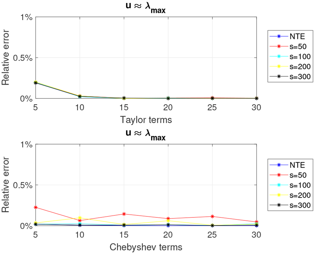
Consider a 5, 000 × 5, 000 random density matrix and let m (the number of terms retained in the Taylor series approximation or the degree of the polynomial used in the Chebyshev polynomial approximation) range between five and 30 in increments of five. Let s, the number of random Gaussian vectors used to estimate the trace, be set to {50,100,200, 300}. Recall that our error bounds for Algorithms 1 and 2 depend on u, an estimate for the largest eigenvalue of the density matrix. We used the power method to estimate the largest eigenvalue (let ${\tilde{\lambda }}_{\max }$ be the estimate) and we set u to ${\tilde{\lambda }}_{\max }$ and $6{\tilde{\lambda }}_{\max }$. Figures 1 and 2 show the relative error (out of 100%) for all combinations of m, s, and u for the Taylor and Chebyshev approximation algorithms. It is worth noting that we also report the error when no trace estimation (NTE) is used in order to highlight that most of the accuracy loss is due to the Taylor/Chebyshev approximation and not the trace estimation.

Fig. 1.

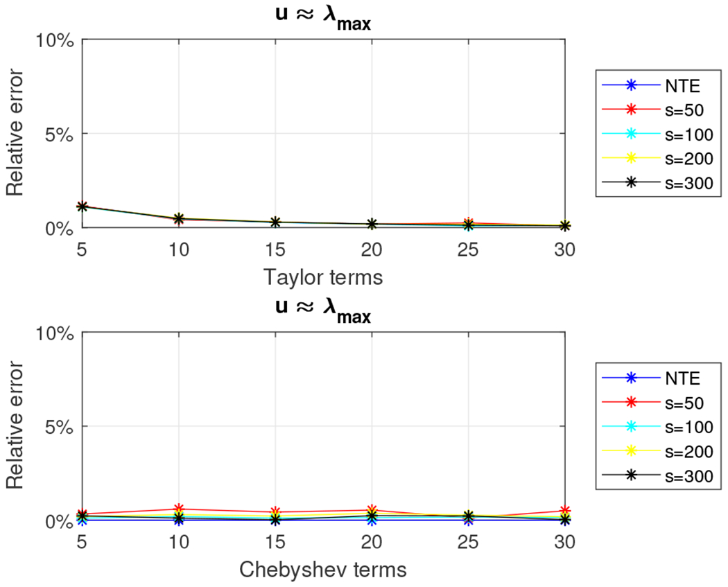
Relative error for 5, 000 × 5, 000 density matrix using the Taylor and the Chebyshev approximation algorithms with $u={\tilde{\lambda }}_{\max }$.

Fig. 2.

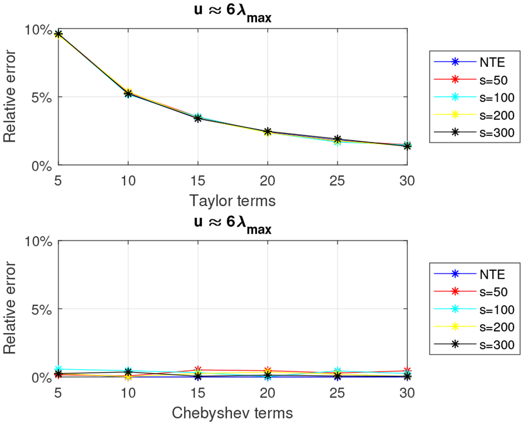
Relative error for 5, 000 × 5, 000 density matrix using the Taylor and the Chebyshev approximation algorithms with $u={\tilde{\lambda }}_{\max }$.

We observe that the relative error is always small, typically close to 1-2%, for any choice of the parameters s, m, and u. The Chebyshev algorithm returns better approximations when u is an overestimate for λ_max while the two algorithms are comparable (in terms of accuracy) where u is very close to λ_max, which agrees with our theoretical results. We also note that estimating the largest eigenvalue incurs minimal computational cost (less than one second). The NTE line (no trace estimation) in the plots serves as a lower bound for the relative error. Finally, we note that computing the exact Von-Neumann entropy took approximately 1.5 minutes for matrices of this size.

The second dataset that we experimented with was a much larger density matrix of size 30, 000 × 30, 000. This matrix was the largest matrix for which the memory was sufficient to perform operations like the full SVD. Notice that since the increase in the matrix size is six-fold compared to the previous one and SVD’s running time grows cubically with the input size, we expect the running time to compute the exact SVD to be roughly 6³ · 90 seconds, which is approximately 5.4 hours; indeed, the exact computation of the Von-Neumann entropy took approximately 5.6 hours. We evaluated both the Taylor and the Chebyshev approximation schemes by setting the parameters m and s to take values in the sets {5, 10, 15, 20} and {50, 100, 200}, respectively. The parameter u was set to ${\tilde{\lambda }}_{\max }$, where the latter value was computed using the power method, which took approximately 3.6 minutes. We report the wall-clock running times and relative error (out of 100%) in Figures 5 and 4.

Fig. 5.

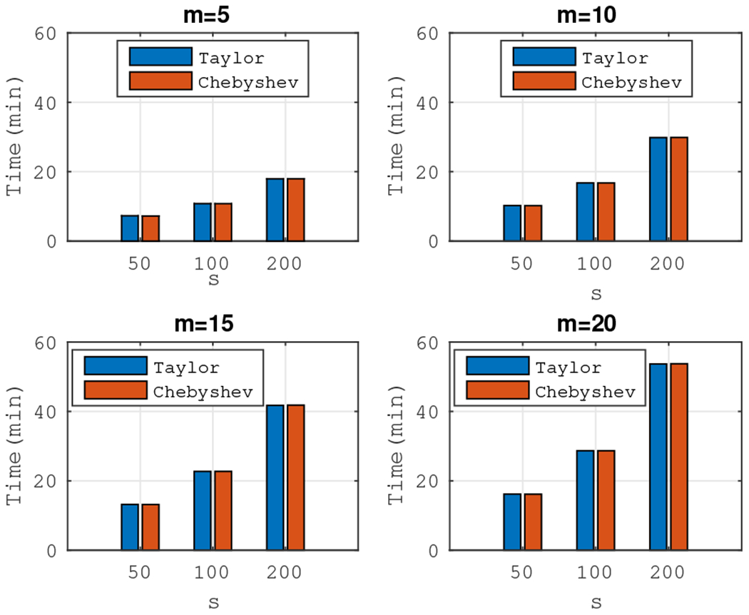
Wall-clock times: Taylor approximation (blue) and Chebyshev approximation (red) for $u={\tilde{\lambda }}_{\max }$. Exact computation needed approximately 5.6 hours.

Fig. 4.

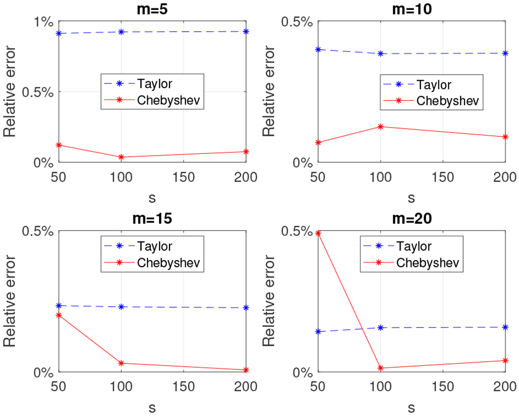
Relative error for 30, 000 × 30, 000 density matrix using the Taylor and the Chebyshev approximation algorithms with $u={\tilde{\lambda }}_{\max }$.

We observe that the relative error is always less than 1% for both methods, with the Chebyshev approximation yielding almost always slightly better results. Note that our Chebyshev-polynomial-based approximation algorithm significantly outperformed the exact computation: e.g., for m = 5 and s = 50, our estimate was computed in less than ten minutes and achieved less than .2% relative error.

The third dataset we experimented with was the tridiagonal matrix from [12, Section 5.1]:

$$\mathbf{A}=\left[\begin{array}{ccccc}2& -1& 0& \dots & 0\\ -1& 2& -1& \ddots & ⋮\\ 0& \ddots & \ddots & \ddots & 0\\ ⋮& \ddots & -1& 2& -1\\ 0& \dots & 0& -1& 2\end{array}\right]$$ (21)

This matrix is the coefficient matrix of the discretized onedimensional Poisson equation:

$$f\left(x\right)=-\frac{d^2{v}_x}{dx}$$

defined in the interval [0, 1] with Dirichlet boundary conditions v(0) = v(1) = 0. We normalize A by dividing it with its trace in order to make it a density matrix. Consider the 5, 000 × 5, 000 normalized matrix A and let m (the number of terms retained in the Taylor series approximation or the degree of the polynomial used in the Chebyshev polynomial approximation) range between five and 30 in increments of five. Let s, the number of random Gaussian vectors used for estimating the trace be set to 50, 100, 200, or 300. We used the formula

$${\lambda }_i=\frac{4}{2n}{\sin }^2\left(\frac{i\pi }{2n+2}\right),i=1,\dots ,n$$ (22)

to compute the eigenvalues of A (after normalization) and we set u to λ_max and 6λ_max. Figures 6 and 7 show the relative error (out of 100%) for all combinations of m, s, and u for the Taylor and Chebyshev approximation algorithms. We also report the error when no trace estimation (NTE) is used.

Fig. 6.

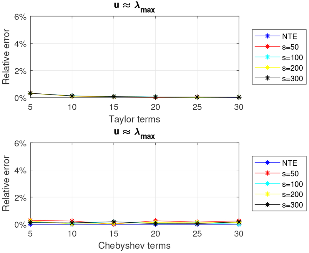
Relative error for 5, 000 × 5, 000 tridiagonal density matrix using the Taylor and the Chebyshev approximation algorithms with u = λ_max.

Fig. 7.

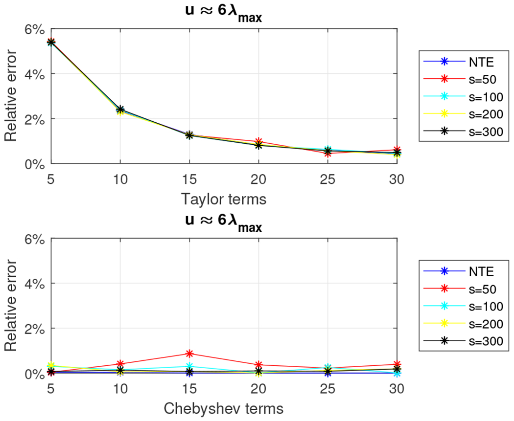
Relative error for 5, 000 × 5, 000 tridiagonal density matrix using the Taylor and the Chebyshev approximation algorithms with u = 6λ_max.

We observe that the relative error is higher than the one observed for the 5, 000 × 5, 000 random density matrix. We report wall-clock running times in Figure 8. The Chebyshev-polynomial-based algorithm returns better approximations for all choices of the parameters and, in most cases, is faster than the Taylor-polynomial-based algorithm, e.g. for m = 5, s = 50 and u = λ_max, our estimate was computed in about two seconds and achieved less than .5% relative error.

Fig. 8.

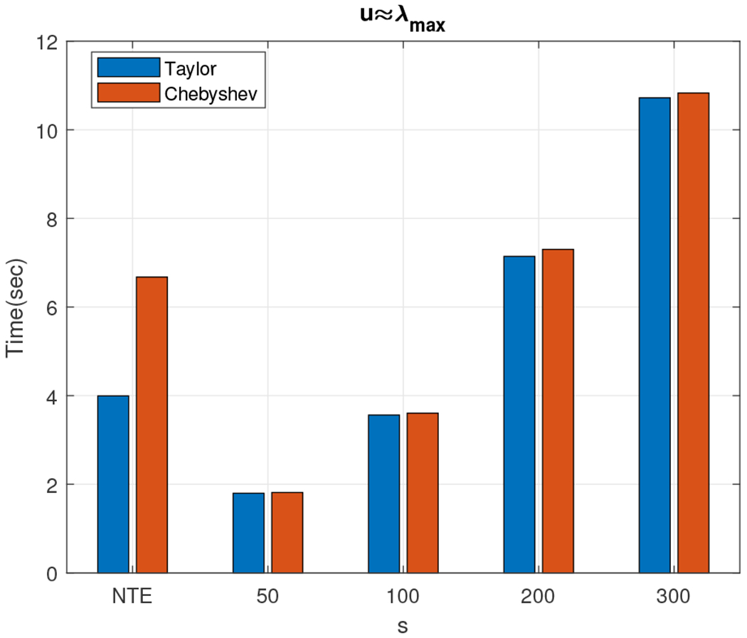
Wall-clock times: Taylor approximation (blue) and Chebyshev approximation (red) for m = 5. Exact computation needed approximately 30 seconds.

We further considered a 10⁸ × 10⁸ tridiagonal matrix of the form of eqn. (21). Although an exact computation of the singular values of A is not feasible (at least with our computational resources), such a computation is not necessary since eqn. (22) provides a closed formula for its eigenvalues and, thus, its entropy. Let m (the number of terms retained in the Taylor series approximation or the degree of the polynomial used in the Chebyshev polynomial approximation) be equal to five or ten and let s, the number of random Gaussian vectors used to estimate the trace be equal to 50 or 100. Figures 9 and 10 show the relative error (out of 100%) and the runtime, respectively, for all combinations of m and s for both the Taylor and Chebyshev approximation algorithms. We observe that in both cases we estimated the entropy in less than ten minutes with a relative error below 0.15%.

Fig. 9.

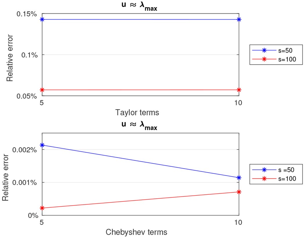
Relative error for the 10⁸ × 10⁸ tridiagonal density matrix using the Taylor and the Chebyshev approximation algorithms with u = λ_max.

Fig. 10.

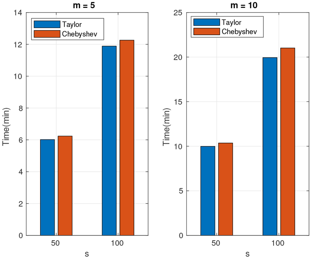
Wall-clock times: Taylor approximation (blue) and Chebyshev approximation (red) for the 10⁸ × 10⁸ triadiagonal density matrix. Exact computation using the Singular Value Decomposition was infeasible using our computational resources.

The fourth dataset we experimented with includes 5, 000 × 5, 000 density matrices whose first top-k eigenvalues follow a linear decay and the remaining 5, 000 – k a uniform distribution. Let k, the number of eigenvalues that follow the linear decay, take values in the set {50, 1000, 3500, 5000}. Let m, the number of terms retained in the Taylor series approximation or the degree of the polynomial used in the Chebyshev polynomial approximation, range between five and 30 in increments of five. Let s, the number of random Gaussian vectors used to estimate the trace, be set to {50, 100, 200, 300}. The estimate of the largest eigenvalue u is set to ${\tilde{\lambda }}_{\max }$. Figures 11 to 14 show the relative error (out of 100%) for all combinations of k, m, s, and u for the Taylor and Chebyshev approximation algorithms.

Fig. 11.

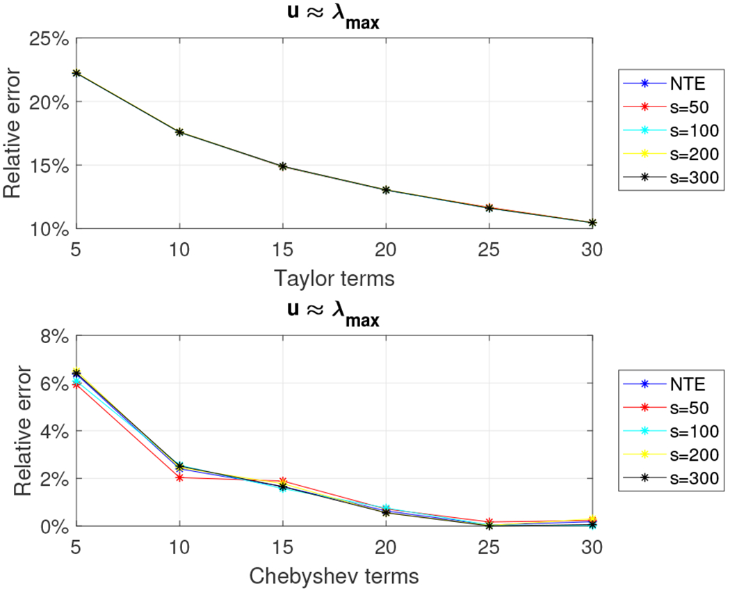
Relative error for 5, 000 × 5, 000 density matrix with the top-50 eigenvalues decaying linearly using the Taylor and the Chebyshev approximation algorithms with u = λ_max.

Fig. 14.

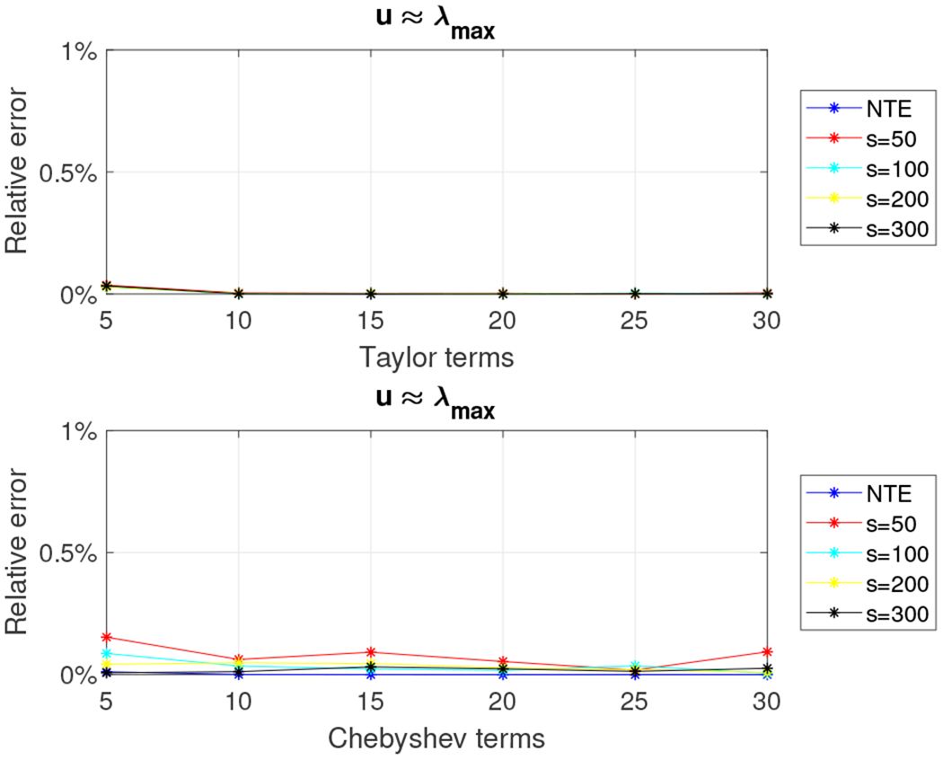
Relative error for 5, 000 × 5, 000 density matrix with the top-5000 eigenvalues decaying linearly using the Taylor and the Chebyshev approximation algorithms with u = λ_max.

We observe that the relative error is decreasing as k increases. It is worth noting that when k = 3,500 and k = 5, 000 the Taylor-polynomial-based algorithm returns better relative error approximation than the Chebyshev-polynomial-based algorithm. In the latter case we observe that the relative error of the Taylor-based algorithm is almost zero. This observation has a simple explanation. Figure 15 shows the distribution of the eigenvalues in the four cases we examine. We observe that for k = 50 the eigenvalues are spread in the interval (10^—2, 10⁻⁴); for k = 1, 000 the eigenvalues are spread in the interval (10⁻³, 10⁻⁴); while for k = 3, 500 or k = 5, 000 the eigenvalues are of order 10⁻⁴. It is well known that the Taylor polynomial returns highly accurate approximations when it is computed on values lying inside the open disc centered at a specific value u, which, in our case, is the approximation to the dominant eigenvalue. The radius of the disk is roughly r = λ_m+1/λ_m, where m is the degree of the Taylor polynomial. If r ≤ 1 then the Taylor polynomial converges; otherwise it diverges. Figure 16 shows the convergence rate for various values of k. We observe that for k = 50 the polynomial diverges, which leads to increased errors for the Taylor-based approximation algorithm (reported error close to 23%). In all other cases, the convergence rate is close to one, resulting in negligible impact to the overall error.

Fig. 15.

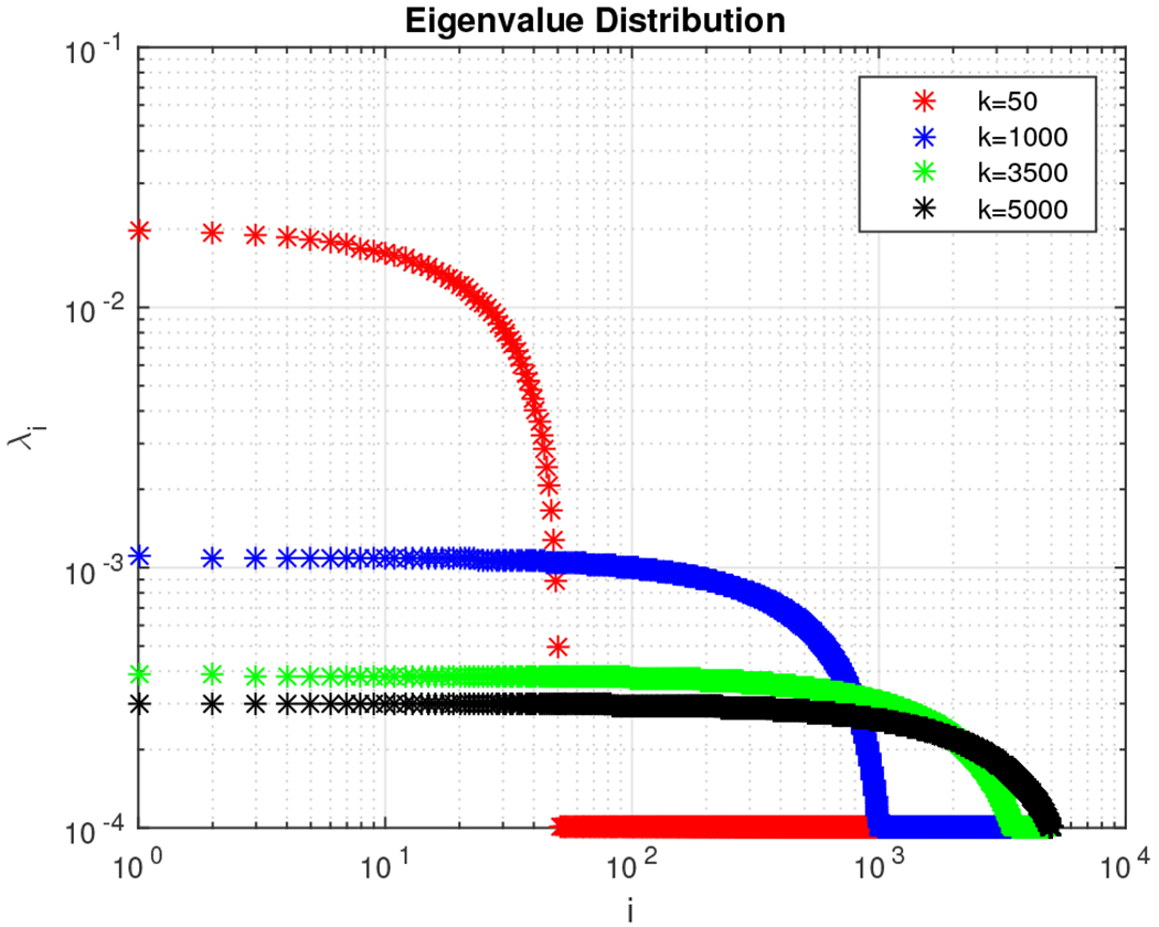
Eigenvalue distribution of 5, 000 × 5, 000 density matrices with the top-k = {50, 1000, 3500, 5000} eigenvalues decaying linearly and the remaining ones (5, 000 – k) following a uniform distribution.

Fig. 16.

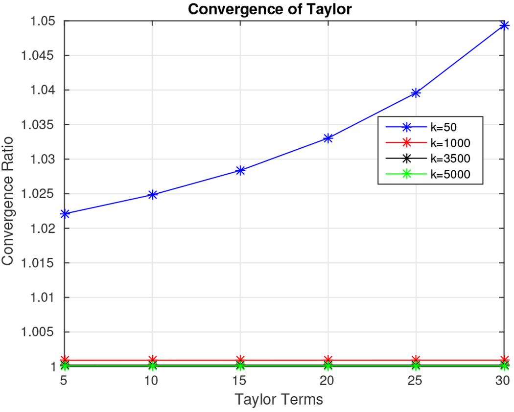
Convergence radius of the Taylor polynomial for the 5, 000 × 5, 000 density matrices with the top-k = {50, 1000, 3500, 5000} eigenvalues decaying linearly and the remaining ones (5, 000 – k) following a uniform distribution.

In all four cases, the Chebyshev-polynomial based algorithm behaves better or similar to the Taylor-polynomial based algorithm. It is worth noting that when the majority of the eigenvalues are clustered around the smallest eigenvalue, then to achieve relative error similar to the one observed for the QETLAB random density matrices, more than 30 polynomial terms need to be retained, which increases the computational time of our algorithms. The increase of the computational time as well as the increased relative error can be justified by the large condition number that these matrices have (remember that for both approximation algorithms the running time depends on the approximate condition number u/l). As an example, for k = 50, the condition number is in the order of hundreds which is significant larger than the roughly constant condition number when k = 5, 000.

B. Empirical Results for the Hermitian Case

Our last dataset is a random 5, 000 × 5, 000 complex density matrix generated using the QETLAB Matlab toolbox. We used the function RandomDensityMatrix of QETLAB and the Haar measure. Let m (the number of terms retained in the Taylor series approximation or the degree of the polynomial used in the Chebyshev polynomial approximation) range between five and 30 in increments of five. Let s, the number of random Gaussian vectors used to estimate the trace, be set to {50, 100, 200, 300}. Figures 17 and 18 show the relative error (out of 100%) for all combinations of m, s, and u for the Taylor-based and Chebyshev-based approximation algorithms respectively.

Fig. 17.

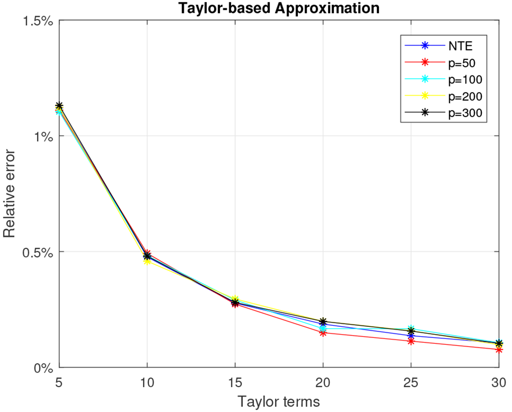
Relative error for 5, 000 × 5, 000 density matrix using the approximation algorithm.

Fig. 18.

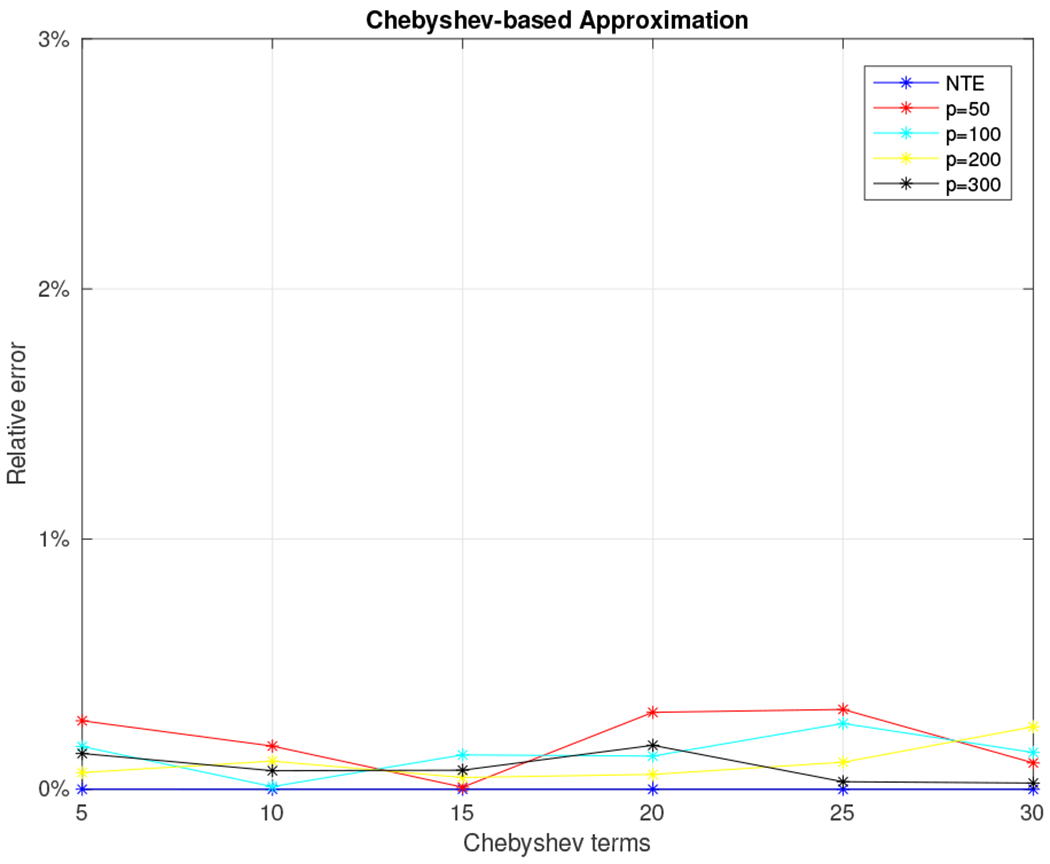
Relative error for 5, 000 × 5, 000 density matrix using the Chebyshev approximation algorithm.

We observe that the relative error is always small, typically below 1%, for any choice of the parameters s and m. The NTE line (no trace estimation) in the plots serves as a lower bound for the relative error. We note that computing the exact Von-Neumann entropy took approximately 52 seconds for matrices of this size. Finally, our algorithm seems to outperform exact computation of the von-Neumann entropy by approximating it in about ten seconds (for the Taylor-based approach) with a relative error of 0.5% using 100 random Gaussian vectors and retaining ten Taylor terms (see Fig. 19) or in about 18 seconds (for the Chebyshev-based approach) with a relative error of 0.2% using 50 random Gaussian vectors and five Chebyshev polynomials (see Fig. 20) .

Fig. 19.

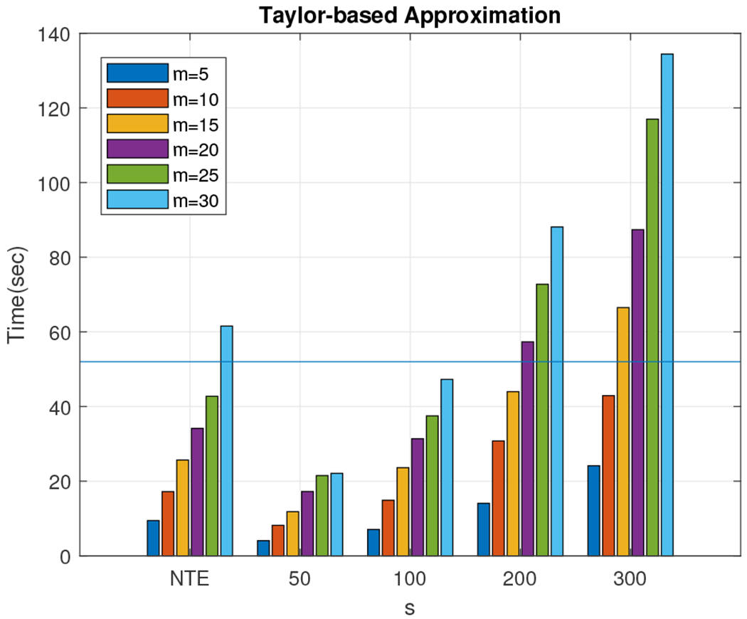
Time (in seconds) to run the Taylor-based algorithm for the 5, 000 × 5, 000 density matrix for all combinations of m and s. Exactly computing the Von-Neumann entropy took approximately 52 seconds, designated by the straight horizontal line in the figure.

Fig. 20.

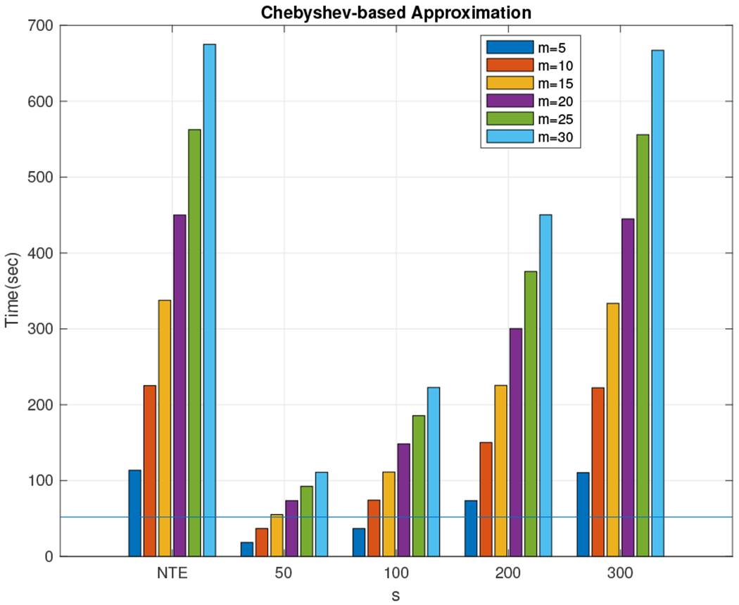
Time (in seconds) to run the Chebyshev-based algorithm for the 5, 000 × 5, 000 density matrix for all combinations of m and s. Exactly computing the Von-Neumann entropy took approximately 52 seconds, designated by the straight horizontal line in the figure.

C. Empirical results for the random projection approximation algorithms

In order to evaluate our third algorithm, we generated low-rank random density matrices (recall that the algorithm of Section V works only for random density matrices of rank k with k ⪡ n). Additionally, in order to evaluate the subsampled randomized Hadamard transform and avoid padding with allzero rows, we focused on values of n (the number of rows and columns of the density matrix) that are powers of two. Finally, we also evaluated a simpler random projection matrix, namely the Gaussian random matrix, whose entries are all Gaussian random variables with zero mean and unit variance.

We generated low rank random density matrices with exponentially (using the QETLAB Matlab toolbox) and linearly decaying eigenvalues. The sizes of the density matrices we tested were 4, 096 × 4, 096 and 16, 384 × 16, 384. We also generated much larger 30, 000 × 30, 000 random matrices on which we only experimented with the Gaussian random projection matrix.

We computed all the non-zero singular values of a matrix using the svds function of Matlab in order to take advantage of the fact that the target density matrix has low rank. The accuracy of our proposed approximation algorithms was evaluated by measuring the relative error; wall-clock times were reported in order to quantify the speedup that our approximation algorithms were able to achieve.

We start by reporting results for Algorithm 5 using the Gaussian, the subsampled randomized Hadamard transform (Algorithm 6), and the input-sparsity transform (Algorithm 7) random projection matrices. Consider the 4, 096 × 4, 096 low rank density matrices and let k, the rank of the matrix, be 10, 50, 100, and 300. Let s, the number of columns of the random projection matrix, range from 50 to 1,000 in increments of 50. Figures 21 and 22 depict the relative error (out of 100%) for all combinations of k and s. We also report the wall-clock running times for values of s between 300 and 450 at Figure 23.

Fig. 21.

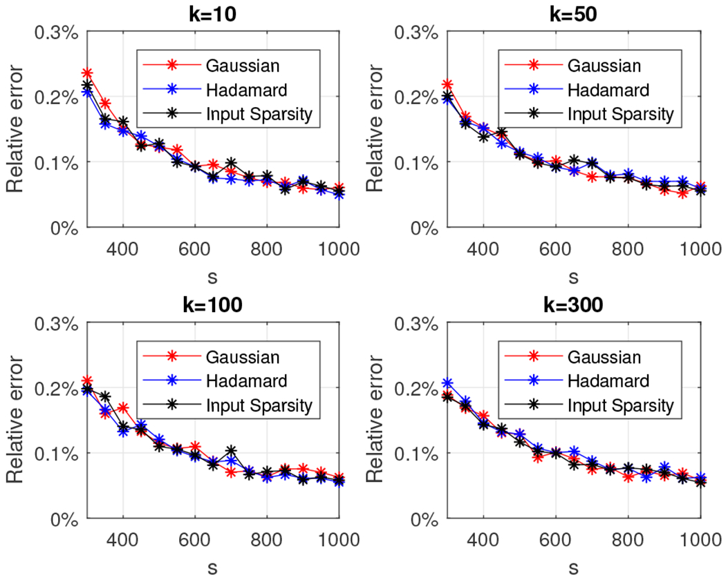
Relative error for the 4, 096 × 4, 096 rank-k density matrix with exponentially decaying eigenvalues using Algorithm 5 with the Gaussian (red), the subsampled randomized Hadamard transform (blue), and the input sparsity transform (black) random projection matrices.

Fig. 22.

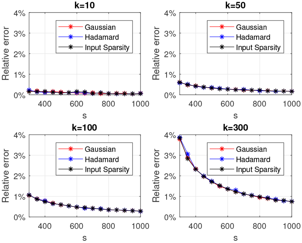
Relative error for the 4, 096 × 4, 096 rank-k density matrix with linearly decaying eigenvalues using Algorithm 5 with the Gaussian (red), the subsampled randomized Hadamard transform (blue), and the input sparsity transform (black) random projection matrices.

Fig. 23.

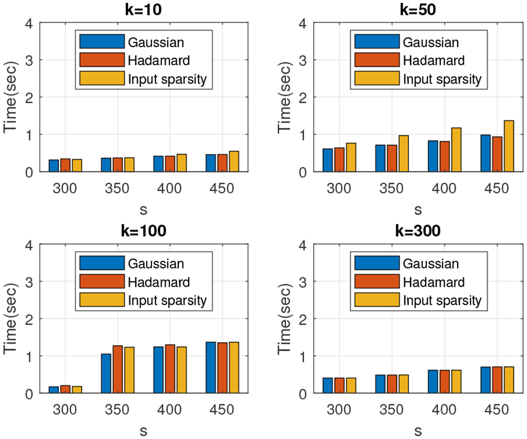
Wall-clock times: Algorithm 5 on 4, 096 × 4, 096 random matrices, with the Gaussian (blue), the subsampled randomized Hadamard transform (red) and the input sparsity transform (orange) projection matrices. The exact entropy was computed in 1.5 seconds for the rank-10 approximation, in eight seconds for the rank-50 approximation, in 15 seconds for the rank-100 approximation, and in one minute for the rank-300 approximation.

We observe that in the case of the random matrix with exponentially decaying eigenvalues and for all algorithms the relative error is under 0.3% for any choice of the parameters k and s and, as expected, decreases as the dimension of the projection space s grows larger. Interestingly, all three random projection matrices returned essentially identical accuracies and very comparable wall-clock running time results. This observation is due to the fact that for all choices of k, after scaling the matrix to unit trace, the only eigenvalues that were numerically non-zero were the 10 dominant ones.

In the case of the random matrix with linearly decaying eigenvalues (and for all algorithms) the relative error increases as the rank of the matrix increases and decreases as the size of the random projection matrix increases. This is expected: as the rank of the matrix increases, a larger random projection space is needed to capture the “energy” of the matrix. Indeed, we observe that for all values of k, setting s = 1, 000 guarantees a relative error under 1%. Similarly, for k = 10, the relative error is under 0.3% for any choice of s.

The running time depends not only on the size of the matrix, but also on its rank, e.g. for k = 100 and s = 450, our approximation was computed in about 2.5 seconds, whereas for k = 300 and s = 450, it was computed in less than one second. Considering, for example, the case of k = 300 exponentially decaying eigenvalues, we observe that for s = 400 we achieve relative error below 0.15% and a speedup of over 60 times compared to the exact computation. Finally, it is observed that all three algorithms returned very comparable wall-clock running time results. This observation could be due to the fact that matrix multiplication is heavily optimized in Matlab and therefore the theoretical advantages of the Hadamard transform did not manifest themselves in practice.

The second dataset we experimented with was a 16,384 × 16,384 low rank density matrix. We set k = 50 and k = 500 and we let s take values in the set {500, 1000, 1500, …, 3000, 3500}. We report the relative error (out of 100%) for all combinations of k and s in Figure 24 for the matrix with exponentially decaying eigenvalues and in Figure 25 for the matrix with linearly decaying eigenvalues. We also report the wall-clock running times for s between 500 and 2,000 in Figure 26. We observe that the relative error is typically around 1% for both types of matrices, with running times ranging between ten seconds and four minutes, significantly outperforming the exact entropy computation which took approximately 3.6 minutes for the rank 50 approximation and 20 minutes for the rank 500 approximation.

Fig. 24.

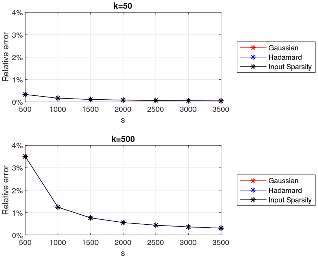
Relative error for the 16, 384 × 16, 384 rank-k density matrix with exponentially decaying eigenvalues using Algorithm 5 with the Gaussian (red), the subsampled randomized Hadamard transform (blue), and the input sparsity transform (black) random projection matrices.

Fig. 25.

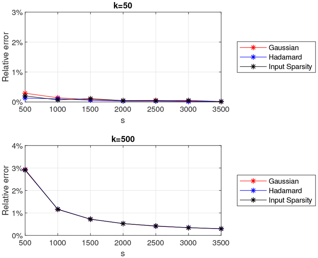
Relative error for the 16, 384 × 16, 384 rank-k density matrix with linearly decaying eigenvalues using Algorithm 5 with the Gaussian (red), the subsampled randomized Hadamard transform (blue), and the input sparsity transform (black) random projection matrices.

Fig. 26.

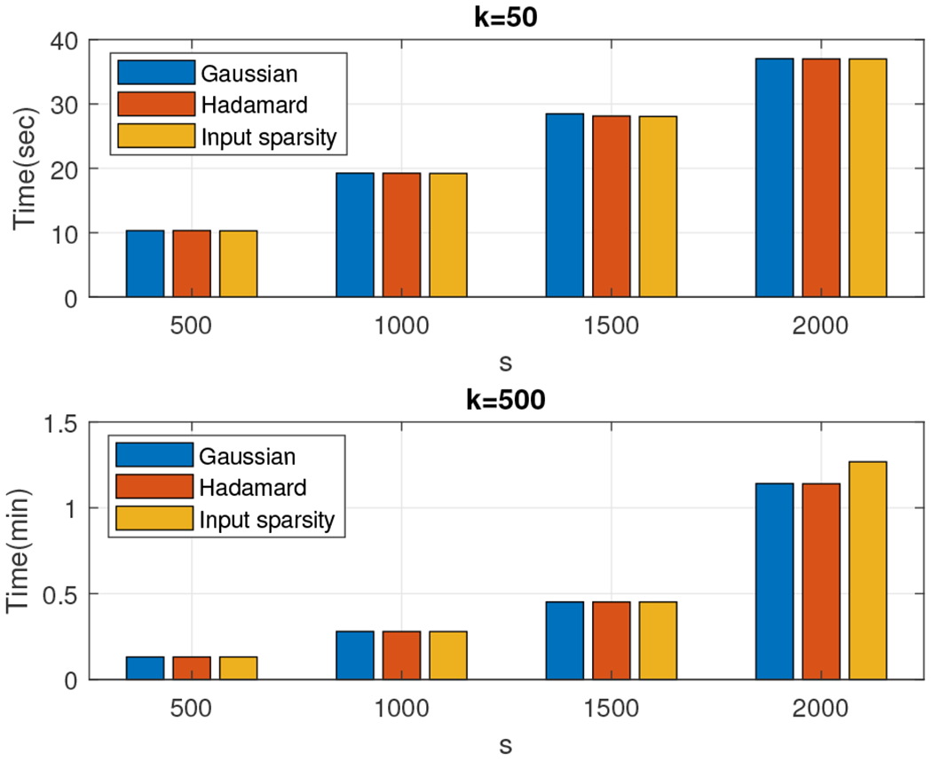
Wall-clock times: Algorithm 5 with the Gaussian (blue), the subsampled randomized Hadamard transform (red) and the input sparsity transform (orange) projection matrices. The exact entropy was computed in 1.6 minutes for the rank 50 approximation and in 20 minutes for the rank 500 approximation.

The last dataset we experimented with was a 30, 000 × 30, 000 low rank density matrix on which we ran Algorithm 5 using a Gaussian random projection matrix. We set k = 50 and k = 500 and we let s take values in the set {500, 1000, 1500, …, 3000, 3500}. We report the relative error (out of 100%) for all combinations of k and s in Figure 27 for the matrix with exponentially decaying eigenvalues and in Figure 28 for the matrix with the linearly decaying eigenvalues. We also report the wall-clock running times for s ranging between 500 and 2, 000 in Figure 29. We observe that the relative error is typically around 1% for both types of matrices, with the running times ranging between 30 seconds and two minutes, outperforming the exact entropy which was computed in six minutes for the rank 50 approximation and in one hour for the rank 500 approximation.

Fig. 27.

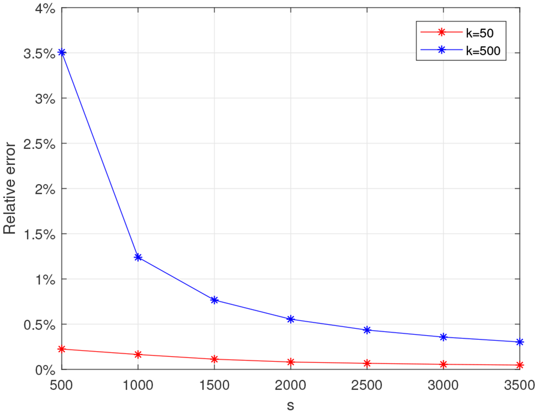
Relative error for the 30, 000 × 30, 000 rank-k density matrix with exponentially decaying eigenvalues using Algorithm 5 with the Gaussian random projection matrix for k = 50 (red) and for k = 500 (blue).

Fig. 28.

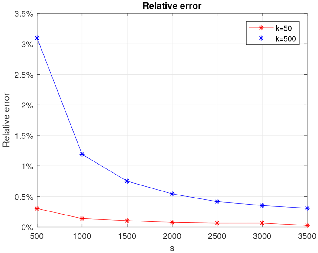
Relative error for the 30, 000 × 30, 000 rank-k density matrix with linearly decaying eigenvalues using Algorithm 5 with the Gaussian random projection matrix for k = 50 (red) and for k = 500 (blue).

Fig. 29.

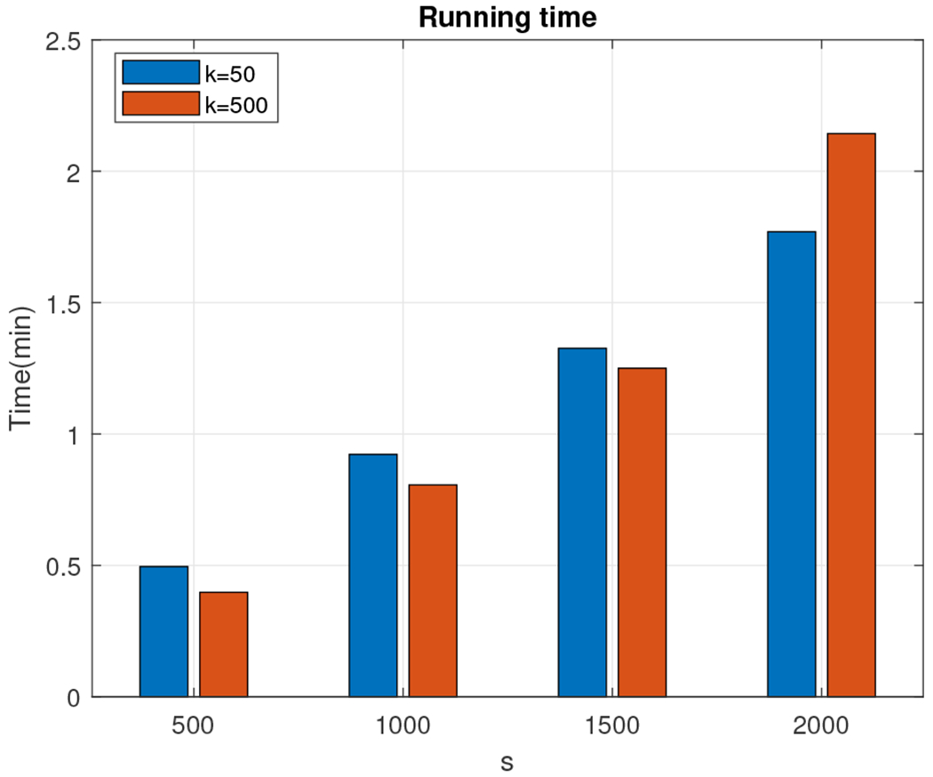
Wall-clock times: rank-50 approximation (blue) and rank-500 approximation (red). Exact computation needed about six minutes and one hour respectively.

VII. Conclusions and open problems

We presented and analyzed three randomized algorithms to approximate the von Neumann entropy of density matrices. Our algorithms leverage recent developments in the RandNLA literature: randomized trace estimators, provable bounds for the power method, the use of random projections to approximate the singular values of a matrix, etc. All three algorithms come with provable accuracy guarantees under assumptions on the spectrum of the density matrix. Empirical evaluations on 30, 000 × 30, 000 synthetic density matrices support our theoretical findings and demonstrate that we can efficiently approximate the von Neumann entropy in a few minutes with minimal loss in accuracy, whereas an the exact computation takes over 5.5 hours.

An interesting open problem would be to consider the estimation of the cross entropy. The cross entropy is a measure between two probability distributions and is particularly important in information theory. Algebraically, it can be defined as $\mathcal{H}(\mathbf{S},\mathbf{R})=-\mathbf{tr}(\mathbf{S}\log \mathbf{R})$, where $\mathbf{S}\in {\mathbb{C}}^{n\times n}$ and $\mathbf{R}\in {\mathbb{C}}^{n\times n}$ are density matrices with a full set of pure states. One can further extend our polynomial-based approaches using the Taylor expansion or the Chebyshev polynomials to approximate the matrix Γ = S log R. The case where both or one of the density matrices have an incomplete set of pure states is an open problem: if R is low-rank, then our first two approaches would not work for the reasons discussed in Section V. However, if the only low rank matrix is S, then our first two approaches would still work: S is only appearing in the trace estimation part, and having eigenvalues equal to zero does not affect the positive semi-definiteness of Γ. When R is of low rank then one might be able to use our random projection approaches to reduce its dimensionality and/or the dimensionality of S.

The most important open problem is to relax (or eliminate) the assumptions associated with our three key technical results without sacrificing our running time guarantees. It would be critical to understand whether our assumptions are, for example, necessary to achieve relative error approximations and either provide algorithmic results that relax or eliminate our assumptions or provide matching lower bounds and counterexamples.

Fig. 3.

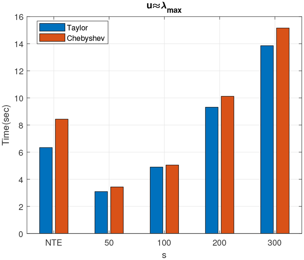
Time (in seconds) to run the approximate algorithms for the 5, 000 × 5, 000 density matrix for m = 5. Exactly computing the Von-Neumann entropy took approximately 90 seconds.

Fig. 12.

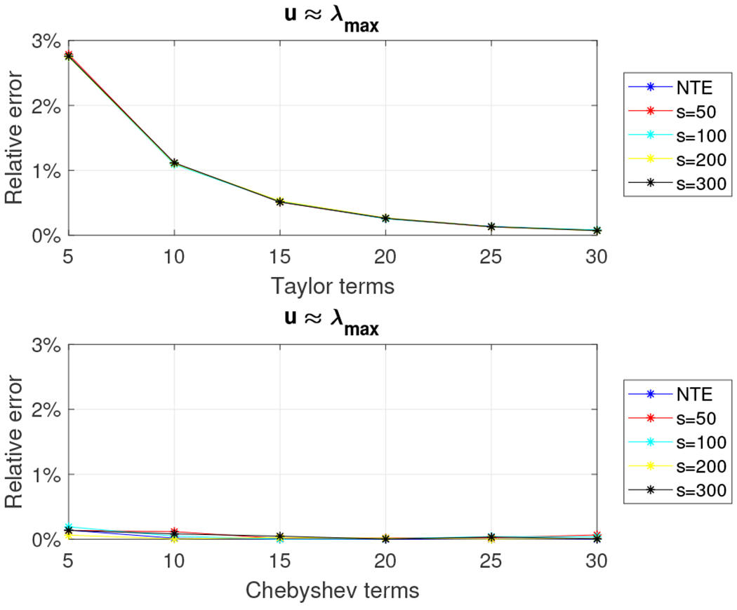
Relative error for 5, 000 × 5, 000 density matrix with the top-1000 eigenvalues decaying linearly using the Taylor and the Chebyshev approximation algorithms with u = λ_max.

Fig. 13.

Relative error for 5, 000 × 5, 000 density matrix with the top-3500 eigenvalues decaying linearly using the Taylor and the Chebyshev approximation algorithms with u = λ_max.

Biographies

Eugenia-Maria Kontopoulou is a Ph.D. candidate with the Computer Science Department at Purdue University. She earned her B. Eng. and M. Eng. from the Computer Science and Informatics Department of University of Patras Greece in 2012. Her current interests lie in the areas of (Randomized) Numerical Linear Algebra with a focus on designing and implementing randomized algorithms for the solution of linear algebraic problems in large-scale data applications.

Gregory Dexter is a current senior at Purdue University majoring in honors statistics and mathematics. He is broadly interested in artificial intelligence and hopes to pursue a PhD focused in this area.

Wojciech Szpankowski is Saul Rosen Distinguished Professor of Computer Science at Purdue University where he teaches and conducts research in analysis of algorithms, information theory, analytic combinatorics, data science, random structures, and stability problems of distributed systems. He held several Visiting Professor/Scholar positions, including McGill University, INRIA, France, Stanford, Hewlett-Packard Labs, Universite de Versailles, University of Canterbury, New Zealand, Ecole Polytechnique, France, the Newton Institute, Cambridge, UK, ETH, Zurich, and Gdansk University of Technology, Poland. He is a Fellow of IEEE, and the Erskine Fellow. In 2010 he received the Humboldt Research Award, in 2015 the Inaugural Arden L. Bement Jr. Award, and in 2020 he was the recipient of the Flajolet Lecture Prize. He published two books: “Average Case Analysis of Algorithms on Sequences”, John Wiley & Sons, 2001, and “Analytic Pattern Matching: From DNA to Twitter”, Cambridge, 2015. In 2008 he launched the interdisciplinary Institute for Science of Information, and in 2010 he became the Director of the newly established NSF Science and Technology Center for Science of Information.

Ananth Grama is the Samuel Conte Professor of Computer Science at Purdue University. His research interests include parallel and distributed computing, large-scale data analytics, and applications in life sciences. Grama received a Ph.D. in computer science from the University of Minnesota. He is a recipient of the National Science Foundation CAREER award and the Purdue University Faculty Scholar Award. Grama is a Fellow of the American Association for the Advancement of Sciences and a Distinguished Alumnus of the University of Minnesota. He chaired the Bio-data Management and Analysis (BDMA) Study Section of the National Institutes of Health from 2012 to 2014. Contact him at ayg@purdue.edu.

Petros Drineas is a Professor at the Computer Science Department of Purdue University. He earned a PhD in Computer Science from Yale University in 2003 and a BS in Computer Engineering and Informatics from the University of Patras, Greece, in 1997. From 2003 until 2016, Prof. Drineas was an Assistant (until 2009) and then an Associate Professor at Rensselaer Polytechnic Institute. His research interests lie in the design and analysis of randomized algorithms for linear algebraic problems, as well as their applications to the analysis of modern, massive datasets, with a particular emphasis on the analysis of population genetics data.

Appendix A. The power method

We consider the well-known power method to estimate the largest eigenvalue of a matrix. In our context, we will use the power method to estimate the largest probability p_i for a density matrix R.

Algorithm 8 requires $\mathcal{O}(\mathit{qt}(n+\mathrm{nnz}(\mathbf{A})))$ arithmetic operations to compute ${\tilde{p}}_1$. The following lemma appeared in [4], building upon [13].

Lemma 14. Let ${\tilde{p}}_1$ be the output of Algorithm 8 with q = ⌈4.82 log(1/δ)⌉ and $t=\lceil \log \sqrt{4n}\rceil$. Then, with probability at least 1 − δ,

$$\frac{1}{6}{p}_1\le {\tilde{p}}_1\le p_1.$$

Algorithm 8.

Power method repeated q times.

• INPUT: SPD matrix $\mathbf{A}\in {\mathbb{R}}^{n\times n}$, integers q, t > 0.

• For j = 1, …, q

1) Pick uniformly at random a vector ${\mathbf{x}}_0^j\{+1,-1{\}}^n$.

2) For i = 1, …, t

– ${\mathbf{x}}_i^j=\mathbf{A}·{\mathbf{x}}_{i-1}^j$.

3) Compute: ${\tilde{p}}_1^j=\frac{{{\mathbf{x}}_t^j}^T\mathbf{A}{\mathbf{x}}_t^j}{{{\mathbf{x}}_t^j}^T{\mathbf{x}}_t^j}$.

• OUTPUT: ${\tilde{p}}_1={\max }_{j=1\dots q}{\tilde{p}}_1^j$.

The running time of Algorithm 8 is $\mathcal{O}((n+\mathrm{nnz}(\mathbf{A}))\log (n)\log (\frac{1}{\delta }))$.

Appendix B. The Clenshaw Algorithm

We briefly sketch Clenshaw’s algorithm to evaluate Chebyshev polynomials with matrix inputs. Clenshaw’s algorithm is a recursive approach with base cases b_m+2(x) = b_m+1(x) = 0 and the recursive step (for k = m, m − 1, …, 0):

$$b_k\left(x\right)={\alpha }_k+2x{b}_{k+1}\left(x\right)-b_{k+2}\left(x\right).$$ (23)

(See Section III for the definition of α_k.) Then,

$$f_m\left(x\right)=\frac{1}{2}\left({\alpha }_0+b_0\left(x\right)-b_2\left(x\right)\right)$$ (24)

Using the mapping x → 2(x/u) − 1, eqn. (23) becomes

$$b_k\left(x\right)={\alpha }_k+2\left(\frac{2}{u}x-1\right)b_{k+1}\left(x\right)-b_{k+2}\left(x\right).$$ (25)

In the matrix case, we substitute x by a matrix. Therefore, the base cases are B_m+2(R) = B_m+1(R) = 0 and the recursive step is

$${\mathbf{B}}_k\left(\mathbf{R}\right)={\alpha }_k{\mathbf{I}}_n+2\left(\frac{2}{u}\mathbf{R}-{\mathbf{I}}_n\right){\mathbf{B}}_{k+1}\left(\mathbf{R}\right)-{\mathbf{B}}_{k+2}\left(\mathbf{R}\right)$$ (26)

for k = m, m − 1, …, 0. The final sum is

$$f_m\left(\mathbf{R}\right)=\frac{1}{2}\left({\alpha }_0{\mathbf{I}}_n+{\mathbf{B}}_0\left(\mathbf{R}\right)-{\mathbf{B}}_2\left(\mathbf{R}\right)\right).$$ (27)

Using the matrix version of Clenshaw’s algorithm, we can now rewrite the trace estimation g^T f_m(R)g as follows. First, we right multiply eqn. (26) by g,

$$\begin{gathered} {\mathbf{B}}_k\left(\mathbf{R}\right)\mathbf{g}={\alpha }_k{\mathbf{I}}_n\mathbf{g}+2\left(\frac{2}{u}\mathbf{R}-{\mathbf{I}}_n\right){\mathbf{B}}_{k+1}\left(\mathbf{R}\right)\mathbf{g}-{\mathbf{B}}_{k+2}\left(\mathbf{R}\right)\mathbf{g}, \\ {\mathbf{y}}_k={\alpha }_k\mathbf{g}+2\left(\frac{2}{u}\mathbf{R}-{\mathbf{I}}_n\right){\mathbf{y}}_{k+1}-{\mathbf{y}}_{k+2}. \end{gathered}$$ (28)

Eqn. (28) follows by substituting y_i = B_i(R)g. Multiplying the base cases by g, we get y_m+2 = y_m+1 = 0 and the final sum becomes

$${\mathbf{g}}^T{f}_m\left(\mathbf{R}\right)\mathbf{g}=\frac{1}{2}\left({\alpha }_0\left({\mathbf{g}}^{\text{T}}\mathbf{g}\right)+{\mathbf{g}}^{\text{T}}\left({\mathbf{y}}_0-{\mathbf{y}}_2\right)\right).$$ (29)

Algorithm 9 summarizes all the above.

Algorithm 9.

Clenshaw’s algorithm to compute g^T f_m(R)g.

1:	INPUT: αi, i = 0, …, m, $\mathbf{R}\in {\mathbb{R}}^{n\times n}$, $\mathbf{g}\in {\mathbb{R}}^n$
2:	Set ym+2 = ym+1 = 0
3:	for k = m, m − 1, …, 0 do
4:	${\mathbf{y}}_k={\alpha }_k\mathbf{g}+\frac{4}{u}{\mathbf{Ry}}_{k+1}-2{\mathbf{y}}_{k+1}-{\mathbf{y}}_{k+2}$
5:	end for
6:	OUTPUT: ${\mathbf{g}}^{\text{T}}{f}_m(\mathbf{R})\mathbf{g}=\frac{1}{2}({\alpha }_0({\mathbf{g}}^{\text{T}}\mathbf{g})+{\mathbf{g}}^{\text{T}}({\mathbf{y}}_0-{\mathbf{y}}_2))$

References

- [1].Golub GH and Van Loan CF, Matrix Computations (3rd Ed.). Baltimore, MD, USA: Johns Hopkins University Press, 1996. [Google Scholar]
- [2].Wihler TP, Bessire B, and Stefanov A, “Computing the Entropy of a Large Matrix,” Journal of Physics A: Mathematical and Theoretical, vol. 47, no. 24, p. 245201, 2014. [Google Scholar]
- [3].Higham NJ, Functions of Matrices: Theory and Computation. Philadelphia, PA, USA: Society for Industrial and Applied Mathematics, 2008. [Google Scholar]
- [4].Boutsidis C, Drineas P, Kambadur P, Kontopoulou E-M, and Zouzias A, “A Randomized Algorithm for Approximating the Log Determinant of a Symmetric Positive Definite Matrix,” Linear Algebra and its Applications, vol. 533, pp. 95–117, 2017. [Google Scholar]
- [5].Avron H and Toledo S, “Randomized Algorithms for Estimating the Trace of an Implicit Symmetric Positive Semi-definite Matrix,” Journal of the ACM, vol. 58, no. 2, p. 8, 2011. [Google Scholar]
- [6].Drineas P and Mahoney MW, “RandNLA: Randomized Numerical Linear Algebra,” Communications of the ACM, vol. 59, no. 6, pp. 80–90, 2016. [Google Scholar]
- [7].Woodruff DP, “Sketching as a Tool for Numerical Linear Algebra,” Foundations and Trends in Theoretical Computer Science, vol. 10, no. 1-2, pp. 1–157, 2014. [Google Scholar]
- [8].Demmel J and Veselic K, “Jacobi’s Method is more Accurate than QR,” SIAM Journal on Matrix Analysis and Applications, vol. 13, no. 4, pp. 1204–1245, 1992. [Google Scholar]
- [9].Johnston N, “QETLAB: A Matlab toolbox for quantum entanglement, version 0.9,” http://qetlab.com, 2016.
- [10].Musco C, Netrapalli P, Sidford A, Ubaru S, and Woodruff DP, “Spectrum Approximation Beyond Fast Matrix Multiplication: Algorithms and Hardness,” 2018. [Online]. Available: http://arxiv.org/abs/1704.04163
- [11].Harvey NJ, Nelson J, and Onak K, “Sketching and streaming entropy via approximation theory,” in IEEE Annual Symposium on Foundations of Computer Science, 2008, pp. 489–498. [Google Scholar]
- [12].Han I, Malioutov D, and Shin J, “Large-scale Log-determinant Computation through Stochastic Chebyshev Expansions,” Proceedings of the 32nd International Conference on Machine Learning, vol. 37, pp. 908–917, 2015. [Google Scholar]
- [13].Trevisan L, “Graph Partitioning and Expanders,” 2011, handout 7.
- [14].Ailon N and Chazelle B, “The Fast Johnson–Lindenstrauss Transform and Approximate Nearest Neighbors,” SIAM Journal on Computing, vol. 39, no. 1, pp. 302–322, 2009. [Google Scholar]
- [15].Drineas P, Mahoney MW, Muthukrishnan S, and Sarlós T, “Faster Least Squares Approximation,” Numerische Mathematik, vol. 117, pp. 219–249, 2011. [Google Scholar]
- [16].Tropp JA, “Improved Analysis of the Subsampled Randomized Hadamard Transform,” Advances in Adaptive Data Analysis, vol. 03, no. 01, p. 8, 2010. [Google Scholar]
- [17].Paul S, Boutsidis C, Magdon-Ismail M, and Drineas P, “Random projections and support vector machines,” in Proceeding of the 16th International Conference on Artificial Intelligence and Statistics, 2013. [Google Scholar]
- [18].Clarkson KL and Woodruff DP, “Low Rank Approximation and Regression in Input Sparsity Time,” in Proceedings of the 45th annual ACM Symposium on Theory of Computing. ACM Press, 2013, pp. 81–90. [Google Scholar]
- [19].Meng X and Mahoney MW, “Low-distortion Subspace Embeddings in Input-sparsity Time and Applications to Robust Linear Regression,” in Proceedings of the 45th annual ACM Symposium on Theory of Computing, 2013, pp. 91–100. [Google Scholar]
- [20].Nelson J and Nguyn HL, “OSNAP: Faster Numerical Linear Algebra Algorithms via Sparser Subspace Embeddings,” in Proceedings of the 46th annual IEEE Symposium on Foundations of Computer Science, 2013. [Google Scholar]