Assessment of the Reproducibility of Postprocessing Dynamic CT Perfusion Data

Abstract

BACKGROUND AND PURPOSE: Commercially available software programs for the conversion of dynamic CT perfusion (CTP) source data into cerebral blood volume (CBV), cerebral blood flow (CBF), and mean transit time (MTT) maps require operators to subjectively define parameters that are used in subsequent postprocessing calculations. Our purpose was to define the variability of CBV, CBF, and MTT values derived from CTP maps generated from the same source data postprocessed by three different CT technologists (CTTs).

METHODS: Raw data derived from dynamic CTP examinations performed in 20 subjects were postprocessed seven times by three experienced CTTs. Parenchymal regions of interest derived from each map (CBV, CBF, and MTT) were compared. The CBF maps generated by each technologist were also qualitatively assessed. Decisions made by each analyzer during postprocessing were assessed.

RESULTS: The intraclass correlation coefficients were 0.73 (95% CI, 0.64–0.81), 0.87 (0.83–0.91) and 0.89 (0.85–0.93), for the CBV, CBF, and MTT parenchymal regions of interest, respectively. All individual correlation coefficients between data sets were significant to a P value <.05. Measurement error, made solely on the basis of different technologists postprocessing the same source data and expressed as the coefficients of variation, were 31%, 30%, and 14% for CBV, CBF, and MTT, respectively. The selection of the arterial input function (AIF) region of interest, venous function region of interest, and preenhancement interval were very reproducible. The technologists differed significantly with respect to the selection of the postenhancement image (PoEI) (P < .01). A retrospective review of the individual CBF maps indicated that variance in the PoEI selection accounted for much of the variation in the qualitative appearance of the CBF maps generated by different technologists. The PoEI was selected to demarcate the baseline of the AIF time-attenuation curve. It is likely that this method of PoEI selection significantly contributed to intra- and interanalyzer variability.

CONCLUSION: There is a high degree of correlation between parenchymal regions of interest derived from CBV, CBF, and MTT maps generated from the same dynamic CTP source data postprocessed by different operators. The level of agreement, however, may not be sufficient to incorporate quantitative values into clinical decision making. Quantitative differences between parenchymal regions of interest were not infrequently manifest as significant differences in the qualitative appearance of the CBF maps. It is likely that, with optimization of postprocessing parameter selection, the degree of variability may be substantially reduced.

The vascular neuroimaging modalities currently in widespread use are almost universally designed to define the macroscopic anatomy of the cerebral vasculature. Clinical decisions are subsequently based on inferences about the underlying physiology at the level of the cerebral microvasculature. Dynamic CT perfusion (CTP) represents an inexpensive, noninvasive, and widely available tool that can be applied to quantitatively measure cerebral blood flow (CBF) (1, 2). Previously, these data were only accessible with oxygen-15 (O-15)–labeled water positron emission tomography (PET) (3). Unfortunately, quantitative O-15 water PET CBF studies are expensive, invasive (requiring an arterial line), and not widely accessible. The growing accessibility of CTP has resulted in its increasing application as a clinical tool for the assessment and management of cerebrovascular disease in individual patients, as well as a research tool for the study of cerebrovascular disease (4).

If quantitative CTP data are to be applied to the study of cerebral perfusion, the technique must be demonstrated to be both precise and accurate. To the best of our knowledge, no study to date has adequately addressed the issue of perfusion in humans. Maps depicting cerebral blood volume (CBV), CBF, and mean transit time (MTT) represent the end result of the postprocessing of source data derived from sequential CT images generated during a dynamic CTP study (5). The precision of CTP data is directly linked to the reproducibility of this postprocessing procedure. Most of the commercially available CTP postprocessing software programs require the operator to subjectively define parameters that are subsequently applied in the calculations, which generate CBV, CBF and MTT maps. The current study was designed to assess the reproducibility of CTP postprocessing performed using one such commercially available software program.

Methods

Patients

Source data from dynamic CTP examinations performed in 20 patients were used in the current study. The population included both inpatients and outpatients who underwent imaging at our institution over a 3-month period. The application of patient data for the current study was approved by the internal review board at our institution (IRB number 02-RA-065).

CTP Technique

CTP source data were derived from sequential scans acquired at the level of the basal ganglia (80 kVp, 200 mA, 4 × 5 mm collimation, 4i cine mode, 45-second scan, data reconstructed at 0.5-second intervals) after the IV administration of 40 mL of Visipaque-320 at 4 mL/s (5-s delay). Source data were reconstructed into two 10-mm-thick contiguous axial images. Data were transferred to a GE Advantage Windows Workstation (GE Medical Systems, Milwaukee, WI). Postprocessing was performed by using CT Perfusion software (GE Medical Systems) with application of the “accurate” CBV, CBF, and MTT algorithms (Fig 1). The commercially available CT Perfusion software used in the current study is based on a deconvolution algorithm (6).

Fig 1.

Example of the selection of postprocessing parameters (15). Dynamic CTP data are derived from 89 sequential contrast-enhanced CT images. A and B are magnified images selected from a series of sequential enhanced CT images performed during a dynamic CTP examination. An AIF is selected by placing a small circular region of interest (1–4 mm²) within the earliest appearing and most densely enhancing artery (usually one of the anterior or middle cerebral arteries). A depicts a small circular region of interest (circle, labeled “1”) placed within the A2 branch of the right anterior cerebral artery. A venous function is selected by placing a circular region of interest (2–8 mm²) within one of the dural venous sinuses. B depicts a small circular region of interest (circle labeled “2”) placed within the posterior third of the superior sagittal sinus/torcula region. The AIF and VF regions of interest define time (image number)–attenuation curves, which depict the time course of the dynamic enhancement of the artery and vein, respectively (C; ordinate: Hounsfield units; abscissa: image number). The AIF curve (labeled “1”) is of smaller amplitude and appears earlier than the VF curve (labeled “2”). The PrEI is defined as the interval from the first image to the image just preceding the upslope of the AIF curve. The vertical dashed line depicts the demarcation for the last image of the PrEI—images 1–13. The PoEI is defined as the first image after the AIF returns to baseline. The vertical dot-dashed line depicts the demarcation for the PoEI—image 58. The selection of the AIF, VF, PrEI, and PoEI represent the four decisions made by the analyst during the postprocessing of CTP data.

Study Design

Three different CT technologists (CTTs), each with more than 2 years of experience postprocessing CTP data for clinical application, participated in the current study. All technologists were originally trained to postprocess CTP data by a single neuroradiologist (S.P.). Technologists were trained to select postprocessing parameters by using the criteria recommended by the software vendor (7).

A neuroradiologist (D.F.) placed three standardized circular region of interest on the gray-scale source images (frontal lobe white matter, basal ganglia, parietal-occipital mixed cortical-subcortical white matter) from each of the 20 patients’ examinations. The central coordinates of each region of interest were recorded in millimeters (anterior-posterior, superior-inferior, and right-left). All circular regions of interest were activated with the images set to a displayed field of view (DFOV) of 12.5 cm. This technique of region of interest activation yielded identical circular regions of interest of standardized diameters. The source images with the neuroradiologist-placed parenchymal regions of interest were saved as a reference for the CTTs to use during postprocessing.

The three participating CTTs independently postprocessed the data sets derived from the 20 dynamic CTP examinations (Table 1). During the first and second postprocessing trials, each of the three technologists processed all 20 examinations, yielding the first six data sets. During a third trial, one technologist processed the 20 examinations a third time, yielding the seventh data set.

TABLE 1:

Experimental Design

	CT Technologist 1	CT Technologist 2	CT Technologist 3
Trial 1	ROI Data Set 1	ROI Data Set 2	ROI Data Set 3
Trial 2	ROI Data Set 4	ROI Data Set 5	ROI Data Set 6
Trial 3	ROI Data Set 7	N/A	N/A

Note—The experiment was composed of three trials of postprocessing. All three technologists participated in the first two trials. Each technologist generated a data set derived from the placement of three predetermined identical circular ROIs on the CBV, CBF, and MTT maps generated by postprocessing the raw dynamic CTP data from the examinations of the same 20 patients (60 points per ROI data set). During the third trial, CT technologist 1 postprocessed the 20 patient data set a third time.

At the outset of postprocessing a given examination, the technologists were instructed to set the DFOV to 12.5 cm and then activate three standardized circular parenchymal regions of interest. These regions of interest were then centered on the predetermined coordinates prospectively designated for the corresponding patient. The central coordinates of each region of interest were recorded to verify concordance with the predetermined values for each patient. Technologists then defined and recorded all parameters used in postprocessing, including arterial input function (AIF) region of interest location, venous function (VF) region of interest location, preenhancement interval (PrEI), and postenhancement image (PoEI) (Fig 1). CBV, CBF, and MTT maps were then generated by using the “accurate” algorithm included in CT Perfusion software. For each session of postprocessing, the values of all parenchymal regions of interest derived from each of the three maps (CBV, CBF, and MTT) were recorded (Table 1). This method yielded a “data set” composed of 60 parenchymal region of interest values (three regions of interest derived from each of 20 patient data sets) for each type of map (CBV, CBF, or MTT). For one trial of processing, each technologist also saved the CBV, CBF, and MTT maps generated for each patient.

Data Analysis

Parenchymal Region of Interest Values: Correlation Analysis

The 60 parenchymal region of interest values derived from CBV, CBF, and MTT maps generated by each technologist during each session of postprocessing were assessed for correlation. Consistency between measurements was estimated by means of a mixed-effects model intraclass correlation analysis using mean square estimates from an analysis of variance. Intraclass correlation analyses were performed after each of the three technologists had postprocessed the 20 patient data sets twice. Data from the final trial (data set 7) were not included in the intraclass correlation analysis. Individual Pearson correlation coefficients were also generated for every possible data set pairing. In addition, data reflecting intra- and interanalyzer variability were grouped and fit to a simple regression line.

Parenchymal Region of Interest Values: Within-Subject Standard Deviation

First, the standard deviations for each parenchymal region of interest were graphed as a function of their corresponding mean region of interest to determine whether measurement error was related to the magnitude of the mean parenchymal region of interest value. All CBV, CBF, and MTT measurement errors were related to the mean values for interanalyzer, intraanalyzer, and pooled data sets, with increasing measurement errors observed with increasing mean region of interest values. For this reason, the data were converted by using a logarithmic transformation (8). After the logarithmic transformation, the measurement errors demonstrated no relationship to the mean values.

The log-transformed data were then analyzed by using a one-way analysis of variance (ANOVA) method to determine the within-subject standard deviation for each parenchymal region of interest (9). This value was squared to yield a within-subject variance for each parenchymal region of interest. The mean of the variances was calculated. The antilog of the square root of the mean variance—the geometric standard deviation (GEOSTD)—was then squared. The GEOSTD² value provides a means to calculate the expected range of measurements distributed about any “true value” of CBV, CBF, or MTT in 95% of cases (see Results below). The coefficient of variation, the ratio of the standard deviation to the mean, was calculated and expressed as a percentage to provide an additional estimate of reliability (10).

CBF Maps: Qualitative Evaluation

All CBF maps were displayed identically by using a graded color scale to depict CBF values ranging from 0 to 100 mL/100 g/min. The CBF values within each of the three major vascular territories (anterior cerebral artery [ACA], middle cerebral artery [MCA], and posterior cerebral artery [PCA]) were graded by a single neuroradiologist (D.F.) by using a scale from 1 to 4: 1) critically decreased (predominantly blue), 2) decreased (green > blue, minimal yellow-red), 3) normal (10%–50% yellow-red), or 4) supranormal CBF (>50% red). Although data from 20 patients were collected, all CBF maps for one patient (n = 3) and one CBF map for another patient (n = 1) were unintentionally deleted from the workstation; thus qualitative analysis was possible for only 56 of 60 CBF maps.

Evaluation of Technologist Decision Making

AIF and VF region of interest locations were recorded and reported for each round of analysis. PrEI and PoEI were assessed for agreement by using a single-variable ANOVA with significance determined by a P value <.05. Differences between the groups were assessed by using a least significant difference method with significance determined by a P value <.01.

Results

Parenchymal Region of Interest Values: Correlation Analysis

The intraclass correlation coefficients were 0.73 (95% confidence intervals, 0.64–0.81), 0.87 (0.83–0.91), and 0.89 (0.85–0.93), for the CBV, CBF, and MTT regions of interest, respectively. Individual Pearson correlation coefficients were calculated for all possible between- and within-analyzer pairings (Table 2). All calculated correlation coefficients were significant to a P value <.001. Simple regression analyses performed on combined intra- and same-trial interanalyzer variability data (Figs 2 and 3) indicated a strong linear relationship in both cases for the CBV, CBF, and MTT measurements.

TABLE 2:

Pearson Product-Moment Correlation Coefficients for CBV, CBF and MTT Maps

A: Cerebral Blood Volume ROIs
	ROI Data Set 1	ROI Data Set 2	ROI Data Set 3	ROI Data Set 4	ROI Data Set 5	ROI Data Set 6	ROI Data Set 7
ROI Data Set 1	1	–	–	–	–	–	–
ROI Data Set 2	0.80	1	–	–	–	–	–
ROI Data Set 3	0.77	0.80	1	–	–	–	–
ROI Data Set 4	0.68	0.79	0.78	1	–	–	–
ROI Data Set 5	0.78	0.87	0.88	0.88	1	–	–
ROI Data Set 6	0.76	0.85	0.86	0.87	0.96	1	–
ROI Data Set 7	0.68	0.71	0.67	0.84	0.76	0.79	1

B: Cerebral Blood Flow ROIs
	ROI Data Set 1	ROI Data Set 2	ROI Data Set 3	ROI Data Set 4	ROI Data Set 5	ROI Data Set 6	ROI Data Set 7
ROI Data Set 1	1	–	–	–	–	–	–
ROI Data Set 2	0.89	1	–	–	–	–	–
ROI Data Set 3	0.85	0.88	1	–	–	–	–
ROI Data Set 4	0.83	0.86	0.86	1	–	–	–
ROI Data Set 5	0.83	0.92	0.92	0.91	1	–	–
ROI Data Set 6	0.91	0.93	0.92	0.89	0.91	1	–
ROI Data Set 7	0.91	0.87	0.84	0.89	0.86	0.93	1

C: Mean Transit Time ROIs
	ROI Data Set 1	ROI Data Set 2	ROI Data Set 3	ROI Data Set 4	ROI Data Set 5	ROI Data Set 6	ROI Data Set 7
ROI Data Set 1	1	–	–	–	–	–	–
ROI Data Set 2	0.86	1	–	–	–	–	–
ROI Data Set 3	0.82	0.92	1	–	–	–	–
ROI Data Set 4	0.90	0.93	0.90	1	–	–	–
ROI Data Set 5	0.85	0.92	0.89	0.93	1	–	–
ROI Data Set 6	0.90	0.97	0.89	0.95	0.92	1	–
ROI Data Set 7	0.88	0.95	0.91	0.97	0.93	0.95	1

Fig 2.

Intraobserver variability. Points composing the region of interest data sets generated by the same observers during different postprocessing trials were paired as ordinate and abscissa values (region of interest data sets 1 versus 4, 4 versus 7, 1 versus 7, 2 versus 5, and 3 versus 6) and graphed as a scatter plot. A simple regression analysis was then performed to fit the data points for (A) CBV (r = 0.77), (B) CBF (r = 0.89), and (C) MTT (r = 0.91). The best fit linear regression line (single short-dash line), 95% confidence intervals for the regression line (paired solid lines), and 95% confidence intervals for the data points (paired long-dash lines) are superimposed on the scatter plot.

Fig 3.

Interobserver variability. Points composing the region of interest data sets generated by the different observers during the same trials were paired as ordinate and abscissa values (region of interest data sets 1 versus 2, 1 versus 3, 2 versus 3, 4 versus 5, 4 versus 6, 5 versus 6) and graphed as a scatter plot. A simple regression analysis was then performed to fit the data points for (A) CBV (r = 0.78), (B) CBF (r = 0.86), and (C) MTT (r = 0.88). The best fit linear regression line (single short-dash line), 95% confidence intervals for the regression line (solid lines), and 95% confidence intervals for the data points (paired long-dash lines) are superimposed on the scatter plot.

Parenchymal Region of Interest Values: Within-Subject Standard Deviations and Coefficients of Variation

The geometric within-subject standard deviations (ie, the logarithmic transformation of the standard deviation) for the CBV, CBF, and MTT measurements were calculated for interanalyzer, intraanalyzer, and pooled data. The squares of these standard deviation values (GEOSTD²) are presented in Table 3A. These values provide a means to quantitatively estimate the error derived from the postprocessing of CTP data. For any given CBF value X, the measured values will lie between X divided by GEOSTD² and X multiplied by GEOSTD² 95% of the time. For example, for CBF value of 20 mL/100 g/min, the measured values would be expected to lie between 11.9 and 33.6 (by using the “pooled” GEOSTD² value of 1.68, which takes into account all observations made by the three technologists). The variation would be slightly greater if interobserver variability were considered in isolation and slightly smaller if only intraobserver variability is considered. These results are depicted graphically in Figure 4.

TABLE 3:

A. GEOSTD2 from Interobserver, Intraobserver, and Pooled Data Sets.
	CBV	CBF	MTT
Interobserver
Trial 1 (DS1 v 2 v 3)	1.66	1.68	1.35
Trial 2 (DS4 v 5 v 6)	1.84	1.80	1.31
Average	1.75	1.75	1.34
Intraobserver
CTT1 (DS1 v 4 v 7)	1.56	1.46	1.30
CTT2 (DS2 v 5)	1.29	1.34	1.30
CTT3 (DS3 v 6)	1.47	1.48	1.30
Average	1.58	1.43	1.30
Pooled (DS1–7)	1.72	1.68	1.31

B. GEOSTD2 derived from inter-observer, intra-observer and pooled data sets for CTT2 and CTT3.
	CBV	CBF	MTT
Interobserver
Trial 1 (DS2 v 3)	1.46	1.52	1.26
Trial 2 (DS5 v 6)	1.22	1.48	1.36
Average	1.35	1.50	1.31
Intraobserver
Average	1.39	1.41	1.30
Pooled (DS2,3,5,6)	1.38	1.46	1.30

Note.—The “average” GEOSTD² values for inter- and intra-observer data sets were calculated from the mean of the variances of the transformed data. The squares of the geometric standard deviations can be used to calculate the range of measurements which may be expected about any given “true value”. This range can be calculated by dividing and multiplying any given “true value” by the GEOSTD² (see Results section for example).

Fig 4.

Distribution of the individual parenchymal region of interest values derived from (A) CBV, (B) CBF, and (C) MTT maps as a function of the average value for each corresponding parenchymal region of interest. Ninety-five percent confidence intervals (solid lines) are defined by the squares of the geometric standard deviations for the data sets. The confidence intervals define the range of measurements that would be expected for a given “true value.” If the data generated by CTT 1 are excluded from the analysis (see Results), the 95% confidence intervals are improved substantially for the (D) CBV and (E) CBF data, with little change in the variability of (F) MTT.

Our data analysis indicated that one analyzer (CTT 1) chose PoEI values that were significantly less than those of the other two analyzers (see below). If this technologist’s data are eliminated from the analysis, the variability attributable to postprocessing improved (Table 3B). In this scenario, for a CBF value of 20 mL/100 g/min, measured values would be expected to lie between 13.7 and 29.2 (by using the “pooled” GEOSTD² value of 1.46, which takes into account all observations made by the remaining two technologists).

The coefficient of variation (CV) (ie, the standard deviation over the mean × 100), provides an additional estimate of the percent error in a given measurement. The CVs for the pooled data (DS1–7) were 30%, 31%, and 14% for CBV, CBF, and MTT, respectively. If the data derived from CTT 1 are discarded, the CVs are 17.5%, 20.8%, and 14% for CBV, CBF, and MTT, respectively.

CBF Maps: Qualitative Evaluation

Although the overall patterns and degree of symmetry of CBF were the same in all cases, the absolute levels of CBF differed. Of 336 vascular distributions (six distributions in 56 maps) assessed, one was critically decreased, 57 were decreased, 209 were normal, and 69 were supranormal. In 33 of 336 vascular distributions, at least one technologist’s map demonstrated “decreased” CBF, whereas one or both of the corresponding CBF maps for the same patient processed by the other two technologists indicated “normal” (n = 29) or “supranormal” (n = 4) flow within the same vascular distribution (Fig 5).

Fig 5.

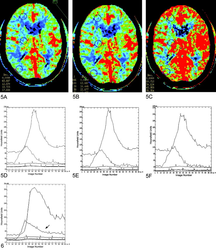
CBF maps generated from a single dynamic CTP data set by three different CTTs (A–C). Dynamic enhancement curves for the AIF (arrowheads) and VF generated by each technologist are depicted (D–F) below the corresponding CBF maps. The three larger circular regions of interest placed in identical locations on each map (frontal lobe white matter, deep gray matter, and temporal lobe mixed cortical-subcortical white matter) represent the prospectively designated parenchymal CBF region of interest measurements made by each technologist. Although these CBF maps were all generated from the same dynamic CTP data set, the results are qualitatively very different. All three maps demonstrate asymmetric CBF within the cerebral hemispheres, left greater than right. A, Map depicts focal regions of decreased CBF within the right posterior temporal lobe and right frontal lobe. B, Map demonstrates a similar region of decreased flow within the right frontal lobe, while the posterior temporal lobe CBF appears more normal (green > blue with some scattered foci or yellow-red). C, Map demonstrates normal (right hemisphere) and supranormal (left hemisphere) CBF without any foci of decreased CBF. The AIF and VF regions of interest were placed within the ACA and posterior third of the superior sagittal sinuses, respectively, by each of the technologists. The corresponding AIF curves (labeled “1”) generated by each technologist are essentially identical. The VF curve (labeled “2”) generated by the third observer (F) does not reach the amplitude of those of the other two observers (D, E). The PrEI chosen by the three technologists were 12, 14, and 11 for A, B, and C, respectively. The PoEI selections chosen by the three technologists were 57, 51, and 42, respectively for A, B, and C, respectively. Thus, while the selections of AIF region of interest, VIF region of interest, and PrEI were very homogeneous between technologists, the selection of the PoEI differed markedly. These data indicate that ambiguity with respect to the selection of the most appropriate PoEI represents a significant source of variability in the calculation of CBF maps.

Fig 6.

Ambiguity of postenhancement image selection. This dynamic enhancement curve (ordinate: Hounsfield units; abscissa: image number (1–89) provides an example of the ambiguity that is frequently involved in the selection of the most appropriate postenhancement image. The downslope of the AIF curve (arrow) is gradual and never completely returns to a baseline over the sequential 89 images. A large range of PoEI selections would be expected if this curve were submitted to multiple different technologists for postprocessing. It is also evident that different selections of the PoEI would result in the exclusion of a variable segment of the downslope of the VF time-attenuation curve from the analysis. The exclusion of segments of the VF time-attenuation curve will result in significant variation in the measured values of CBV and CBF, with larger values calculated when larger segments of the VF curve are excluded from the analysis.

Evaluation of Technologist Decision Making

The selection of both the AIF and VF regions of interest were very reproducible both between and within technologists. Complete concordance in AIF and VF region of interest placement was observed across all seven data sets in 14/20 and 18/20 patients, respectively. The selection of the PrEI also was very reproducible, with no significant differences observed either between or within technologists (P = .52). The technologists differed significantly with respect to the selection of the PoEI (P < .001). A retrospective review of the individual CBF maps indicated that variance in the PoEI selection accounted for much of the variation in the qualitative appearance of the CBF maps generated by different technologists (Fig 5).

Discussion

Cerebral perfusion imaging represents an important extension of the current modalities available for the assessment of the status of the cerebral vasculature (4). Dynamic CTP has significant advantages over the other existing techniques that have been applied to the study of cerebral perfusion. CTP is relatively inexpensive, noninvasive, rapid, and widely accessible (11). CTP also provides quantitative measures of several parameters of cerebral perfusion simultaneously—CBV, CBF, and MTT.

The accepted criterion standard for the measurement of CBF is quantitative O-15 water PET (3); however, the routine application of this technique is limited by inaccessibility, significant cost, and the invasive nature of the examination, which requires the placement of an arterial line and continuous sampling of the arterial concentration of radiotracer. In contrast, the acquisition of CTP data is no more complex than the performance of a standard contrast-enhanced CT scan of the brain. The collected raw data can be rapidly (5–10 minutes) postprocessed either by a CTT or radiologist to produce CBV, CBF, and MTT maps by using commercially available software. Thus, CTP technology is currently accessible to any clinician practicing in a hospital with a helical CT scanner and the appropriate software. This evolution could potentially have a rapid and widespread impact on the management of common vascular problems of the central nervous system (such as carotid stenosis, intracranial atheromatous disease, cerebral vasospasm, and acute stroke). In addition, if validated as both accurate and precise, CTP would likewise represent a highly accessible research tool for the investigation of the pathophysiology and management of cerebrovascular disease.

To accept a new technique for application in the clinical or research setting, the technique must be demonstrated to be reliable with a high degree of precision and accuracy. The precision or reproducibility of CTP data can be considered on multiple levels. Reproducibility must be present at the level of neuroradiologist image interpretation, data postprocessing, and data acquisition. With the exception of neuroradiologist image interpretation, which has been addressed by Eastwood et al (12), no study has assessed the other components of CTP reproducibility. After reproducibility is verified, accuracy can be established by comparing CTP data to the available criterion standard, O-15-labeled water PET imaging. The current study was designed to assess the reproducibility of the postprocessing of dynamic CTP data into CBV, CBF, and MTT maps.

The present data indicate a high level of correlation both between and within technologists postprocessing the same raw CTP data into CBV, CBF, and MTT maps. Regression analyses for intra- and interanalyzer comparisons demonstrate a strong linear relationship with a high level of significance. It is important, however, to note that correlation analyses reflect only the strength of the association between data points and, correspondingly, a correlation coefficient does not represent a measure of reproducibility or agreement (13). The within-subject standard deviation represents a more appropriate method for the analysis of agreement between measurements (8). For cases in which the error in a measurement is related to the mean, a logarithmic transformation of the data is required before calculating the within-subject standard deviation (9). This method of analysis produces a dimensionless ratio (the geometric within-subject standard deviation) from which the range of measured values expected for a given “true value” can be estimated.

The calculated geometric within-subject standard deviations for CBV, CBF, and MTT regions of interest values indicate a clinically significant level of variability. Clinical significance is best defined for CBF. O-15 water PET studies in humans have indicated that CBF levels below 15 mL/100 g/min are inadequate to preserve tissue viability, and levels above 19 mL/100 g/min represent the lowest CBF adequate to maintain normal cerebral function (3). Changes in EEG activity have been documented to occur when CBF levels fall below 17 mL/100 g/min (14). Studies in primates have produced similar results with CBF less than 10 mL/100 g/min producing infarction, whereas CBF ranging between 10 and 20 mL/100 g/min produced reversible ischemia (15). The current data indicate that, on the basis of postprocessing variability alone, if the true CBF value is 20 mL/100 g/min, measurements of CBF can be reasonably expected to vary by approximately ±7–10 mL/100 g/min about this value.

This variability was also reflected when the CBF maps generated by different observers were qualitatively evaluated. While the general patterns of CBF were the same, significant differences in the absolute level of CBF were observed in some cases (Fig 5). In some cases, these differences were potentially clinically significant, with one technologist generating maps demonstrating areas of decreased perfusion and another technologist postprocessing the same data generating maps that demonstrate normal perfusion to the same areas.

Reproducibility rests on establishing homogeneity with respect to the manner in which technologists define variables during postprocessing. The commercially available software used in the current study required four decisions to be made by the analyzer (Fig 1): AIF region of interest, VF region of interest, PrEI, and PoEI. All participating CTTs were trained by a single neuroradiologist (S.P.) to analyze dynamic CTP data, in an attempt to achieve the highest degree of uniformity with respect to postprocessing. The guidelines established for the postprocessing of the CTP data were those recommended by the software vendor (7).

Technologists were instructed to choose the earliest appearing and most dense arterial vessel for the AIF region of interest and to place a small circular region of interest (1–4 mm²) within the central portion of the vessel. AIF region of interest placement was to be performed by using the smallest possible field of view to reduce the potential for volume averaging with adjacent brain. In our retrospective review of AIF selection, AIF location was very homogeneous both between and within technologists with 100% agreement across all seven data sets in 14 of 20 subjects. Variations in the qualitative appearance of CBF maps appeared to be attributable primarily to differences in AIF selection (eg, MCA versus ACA placement) in only three cases however, although the current experiment was designed to identify cases is which technologists chose different vessels for AIF region of interest placement, variations in the position of the regions of interest within the same vessels could not be determined. Because of the phenomenon of volume averaging, it is possible that such differences could significantly contribute to map variability in cases in which the same AIF vessel was selected.

Technologists were instructed to choose the posterior third of the superior sagittal sinus or torcula whenever possible for the VF. The region of interest placement was performed on the smallest possible field of view with windows adjusted to clearly demonstrate a demarcation between the contrast material-containing venous sinus and the adjacent calvaria and brain in an attempt to decrease the potential for volume averaging. Technologists defined small circular regions of interest (2–8 mm²) to be placed within the central portion of the sinus. VF selection appeared to be very straightforward with complete agreement across all seven data sets in 18 of 20 subjects. In those cases in which there was incomplete agreement, one or more of the technologists had placed the VF region of interest within a portion of the distal transverse sinus adjacent to the torcula. In no case did a technologist choose the straight sinus or one of the deep cerebral veins. In no case was variation in the qualitative appearance of the CBF maps attributed to differences in the vessel selected for VF region of interest placement. As with the AIF region of interest placement, however, differences attributable to minor variations in VF region of interest placement would not be detectable by the current experimental design.

Technologists were instructed to choose the PrEI to span from image one of the acquisition to the image preceding the onset of the upslope of the AIF. This selection of the most appropriate PrEI also appeared to be straightforward, because a high degree of reproducibility was observed both between and within technologists. A qualitative review of the configuration of the AIF curves demonstrated an abrupt onset of the upslope against a background of little baseline variability in most cases. The morphology of the upslope of the AIF dynamic enhancement curve functioned to make the selection of the most appropriate PrEI relatively unambiguous. In only one case did a difference in the selection of the PrEI appear to affect the qualitative appearance of the CBF maps.

Technologists were instructed to choose the PoEI as the image defining the point at which the AIF dynamic enhancement curve returned to baseline. The selection of the most appropriate PoEI represented the most important source of variability in our study with significant differences in PoEI selection observed between technologists. One technologist chose significantly earlier images for the PoEI in comparison to the other two technologists. When the data sets generated by this technologist (CTT 1) were excluded from the analysis, the variability in the CBV and CBF data improved. A retrospective review of those CBF maps with the greatest degree of variation frequently demonstrated that PoEI selection was the only variable that differed significantly between technologists. This variation can be attributed to the ambiguity inherent in choosing the most appropriate PoEI in many cases. In contrast to the AIF upslope, the downslope of the AIF curve is frequently gradual (rather than abrupt) and approaches a baseline with a considerable level of noise (Fig 6). As a result, the exact terminis of the downslope is frequently difficult to define. The quantitative CBV and CBF values are normalized to the integrated area under the VF time-attenuation curve. Therefore, the calculated CBV and CBF values are inversely proportional to the area under the VF time-attenuation curve. Because data collected at time points beyond the PoEI are excluded from the deconvolution calculations, the selection of the PoEI after the terminus on the AIF curve frequently excludes from the analysis a significant portion of the tail of the VF curve. Correspondingly, as earlier PoEIs are selected, greater areas under the VF curve are excluded from the analysis and the calculated CBV and CBF values are greater. This phenomenon accounts for the marked variability observed with even small changes in the selection of the PoEI.

To improve the reproducibility in CTP, CTTs and physicians analyzing data must achieve a high degree of uniformity with respect to the selection of the four variables that must be defined during postprocessing. Although this uniformity can be easily achieved for AIF region of interest, VF region of interest, and PrEI selections, the PoEI selection appears to be more problematic because of the configuration of the downslope of the AIF. This problem may be reduced in two ways. First, the PoEI should be chosen after the terminus of the VF time-attenuation curve rather than the AIF time-attenuation curve. PoEI selections that are close to, or incorporate, a portion of the downslope of the VF curve generate the highest degree of variability in subsequent CBF values. Choosing the PoEI after the terminus of the VF time-attenuation curve will prevent the exclusion of data points along the downslope of the VF curve. For examinations in which the time-attenuation curve has not returned to baseline during the 45-s scanning time period, the last image should be chosen for the PoEI. In general, the selection of a later image for the PoEI is preferable to an early image, excluding those cases in which a defined recirculation peak is observed. The incorporation of a recirculation peak into the analyzed data set can lead to erroneous results. Second, the contrast material bolus characteristics should be optimized by placing an 18-gauge antecubital IV and injecting the contrast material bolus at a high rate (4 mL/s). We are currently investigating the utility of a dual injector (with a saline bolus injected as a chaser to follow the initial contrast bolus) as means of improving bolus continuity by increasing the rate of transit of the terminis of the contrast material bolus through the venous system. We expect that optimization of the contrast material bolus characteristics will be manifest as an improvement in reproducibility by reducing noise in the baseline after the bolus and reducing the number of examinations in which the venous curve does not return to baseline over the 45-s acquisition.

There are several significant limitations of the current study. First, all data analysis was performed by using a single commercially available software program (CT Perfusion, GE Medical Systems) that uses a deconvolution algorithm to calculate CTP maps. It is possible that other software programs and/or other mathematical algorithms designed for the analysis of dynamic CTP data may yield different degrees of variability. This is particularly true of software programs in which the selection of the postprocessing parameters is either partially or completely automated. Second, although the location of the parenchymal regions of interest was strictly controlled in the current study by requiring documentation of the central position of each parenchymal region of interest by the technologists, minor variations in the positions of the parenchymal regions of interest were identified. As a result, some fraction of the observed variability may be attributable to small differences in parenchymal region of interest location. In light of the comparatively large area (>175 mm²) of the parenchymal regions of interest, however, the minimal differences in the documented parenchymal region of interest positions are unlikely to have accounted for significant variance in the data. Third, our assessment of the AIF and VF region of interest selection was based on documentation of the vessel chosen. Region of interest size and region of interest position within the target vessel were not tracked. It is possible that small variations in region of interest position within a vessel or region of interest size could potentially result in differences in the characteristics of the dynamic enhancement curves that could subsequently affect not only the selection of the PrEI and PoEI, but ultimately the calculated CBV, CBF and MTT values. Thus, although AIF and VF selection appeared relatively homogeneous in our study, both between and within technologists, these variables cannot be completely discounted as potential sources of variability.

The current data indicate that there are important limitations with respect to the interpretation and application of CTP data. Although CTP data are adequate to define asymmetry in perfusion between vascular distributions, there are significant limitations with respect to the ability to quantitate CBF with a level of reproducibility sufficient to guide clinical decisions. This limitation is particularly important in those cases in which a cerebrovascular disease process is bilateral or diffuse and, subsequently, there is no “normal” region of brain to use as a reference. Such examples would include patients with diffuse intracranial atheromatous disease and patients with diffuse cerebral vasospasm.

Conclusion

There is a high degree of correlation both between and within technologists postprocessing dynamic CTP source data into CBV, CBF, and MTT maps; however, the level of agreement at our institution is currently not sufficient to allow quantitative data derived from CTP maps to be used for clinical decision making. By optimizing the uniformity of decision making in postprocessing (particularly the selection of the PoEI) and improving the characteristics of the contrast bolus, it is likely that substantial improvements in reproducibility can be achieved.

References

- 1.Cenic A, Nabavi DG, Craen RA, et al. Dynamic CT measurement of cerebral blood flow: a validation study. AJNR Am J Neuroradiol 1999;20:63–73 [PubMed] [Google Scholar]
- 2.Nabavi DG, Cenic A, Craen RA, et al. CT assessment of cerebral perfusion: experimental validation and initial clinical experience. Radiology 1999;213:141–149 [DOI] [PubMed] [Google Scholar]
- 3.Powers WJ, Grubb RL, Darriet D, Raichle ME. Cerebral blood flow and cerebral metabolic rate of oxygen requirements for cerebral function and viability in humans. J Cereb Blood Flow Metab 1985;5:600–608 [DOI] [PubMed] [Google Scholar]
- 4.Walker MT, Deshmukh S, Harbison DL, Partovi S. CT perfusion imaging. BNI Quarterly 2001;17:15–27 [Google Scholar]
- 5.Eastwood JD, Lev MH, Provenzale JM. Perfusion CT with iodinated contrast material. Am J Radiol 2003;180:3–15 [DOI] [PubMed] [Google Scholar]
- 6.Wintermark M, Maeder P, Thiran JP, et al. Quantitative assessment of regional cerebral blood flows by perfusion CT studies at low injection rates: a critical review of the underlying theoretical models. Eur Radiol 2001;11:1220–1230 [DOI] [PubMed] [Google Scholar]
- 7.Technical Publication Direction 22897250–100. CT Perfusion 3 Quick Step Guide. Revision 4. GE Medical Systems, November2002
- 8.Bland JM, Altman DG. Transformations, means and confidence intervals. BMJ 1996;312:1079. [DOI] [PMC free article] [PubMed] [Google Scholar]
- 9.Bland JM, Altman DG. Measurement error. BMJ 1996;313:744. [DOI] [PMC free article] [PubMed] [Google Scholar]
- 10.Bland JM, Altman DG. Measurement error proportional to the mean. BMJ 1996;313:106. [DOI] [PMC free article] [PubMed] [Google Scholar]
- 11.Eastwood JD, Provenzale JM, Hurwitz LM, Lee TY. Practical injection rate CT perfusion imaging: deconvolution derived hemodynamics in a case of stroke. Neuroradiology 2001;43:223–226 [DOI] [PubMed] [Google Scholar]
- 12.Eastwood JD, Lev MH, Azhari T, et al. CT Perfusion scanning with deconvolution analysis: pilot study in patients with acute middle cerebral artery stroke. Radiology 2002;222:227–236 [DOI] [PubMed] [Google Scholar]
- 13.Bartko JJ, Carpenter WT. On the methods and theory of reliability. J Nerv Mental Dis 1976;163:307–317 [DOI] [PubMed] [Google Scholar]
- 14.Sundt TM, Sharbrough FS, Anderson RE, Michenfelder JD. Cerebral blood flow measurements and electroencephalograms during carotid endarterectomy. J Neurosurg 1974;41:310–320 [DOI] [PubMed] [Google Scholar]
- 15.Jones TH, Morawetz RB, Crowell RM, et al. Thresholds of focal cerebral ischemia in awake monkeys. J Neurosurg 1981;54:773–782 [DOI] [PubMed] [Google Scholar]