Radiomics for Distinguishing Myocardial Infarction from Myocarditis at Late Gadolinium Enhancement at MRI: Comparison with Subjective Visual Analysis

Abstract

Purpose

To evaluate whether radiomics features of late gadolinium enhancement (LGE) regions at cardiac MRI enable distinction between myocardial infarction (MI) and myocarditis and to compare radiomics with subjective visual analyses by readers with different experience levels.

Materials and Methods

In this retrospective, institutional review board–approved study, consecutive MRI examinations of 111 patients with MI and 62 patients with myocarditis showing LGE were included. By using open-source software, classification performances attained from two-dimensional (2D) and three-dimensional (3D) texture analysis, shape, and first-order descriptors were compared, applying five different machine learning algorithms. A nested, stratified 10-fold cross-validation was performed. Classification performances were compared through Wilcoxon signed-rank tests. Supervised and unsupervised feature selection techniques were tested; the effect of resampling MR images was analyzed. Subjective image analysis was performed on 2D and 3D image sets by two independent, blinded readers with different experience levels.

Results

When trained with recursive feature elimination (RFE), a support vector machine achieved the best results (accuracy: 88%) for 2D features, whereas linear discriminant analysis (LDA) showed the highest accuracy (85%) for 3D features (P <.05). When trained with principal component analysis (PCA), LDA attained the highest accuracy with both 2D (86%) and 3D (89%; P =.4) features. Results found for classifiers trained with spline resampling were less accurate than those achieved with one-dimensional (1D) nearest-neighbor interpolation (P <.05), whereas results for classifiers trained with 1D nearest-neighbor interpolation and without resampling were similar (P =.1). As compared with the radiomics approach, subjective visual analysis performance was lower for the less experienced and higher for the experienced reader for both 2D and 3D data.

Conclusion

Radiomics features of LGE permit the distinction between MI and myocarditis with high accuracy by using either 2D features and RFE or 3D features and PCA.

© RSNA, 2019

Supplemental material is available for this article.

Summary

Radiomics features, identified through machine learning, help distinguish myocardial infarction from myocarditis on the basis of late gadolinium enhancement at MRI with high accuracy.

Key Points

• ■ A radiomics approach with machine learning trained with regions of late gadolinium enhancement on cardiac MR images enables the distinction between myocardial infarction and myocarditis with high accuracy.

• ■ Two-dimensional radiomics features proved to be more discriminating than three-dimensional features for making the distinction when using recursive feature elimination.

• ■ The radiomics approach is more accurate than a human reader performing subjective visual analysis with less experience and slightly less accurate than a reader with advanced experience in cardiovascular imaging.

Introduction

Cardiac MRI is the reference imaging modality for assessing myocardial anatomy and function by providing accurate and reproducible measures of both left and right ventricles in a noninvasive way (1,2). Late gadolinium enhancement (LGE) at cardiac MRI has become the standard for detecting and characterizing myocardial scar as the result of myocardial infarction (MI). LGE also occurs in other myocardial diseases such as inflammation of the myocardium (ie, myocarditis), where regions of contrast enhancement in the myocardium can be found (3).

MI typically results in subendocardial or transmural LGE, which is located in a region consistent with the perfusion territory of an epicardial coronary artery. In contrast, myocarditis shows a predominant subepicardial or intramural location of LGE, although transmural patterns of enhancement might occur. In clinical routine, LGE regions are analyzed in a visual, qualitative way, which may suffer from intra- and interobserver variability. In cases with a transmural pattern, the differentiation between MI and myocarditis on the basis of LGE alone may be difficult. Under certain circumstances, the differentiation of patients with MI and those with myocarditis can be further complicated when clinical information and patient history are limited (4), or patients with both diseases present in a similar way (5). Thus, quantitative measures helping to make this distinction might be beneficial.

Thus far, only a few studies have evaluated the potential of texture analysis and machine learning in cardiac imaging (6–10) when excluding automatic segmentation techniques. Some of these studies performed texture analysis on cardiac MR or CT images for detecting normal and nonviable myocardial segments (6,7), whereas others focused on MI and aimed to identify left ventricular myocardial scar on nonenhanced cine MR images (8). Only one of these studies (6) went beyond two-dimensional (2D) features, adding time information in the feature extraction step, and, to our knowledge, none assessed the potential of three-dimensional (3D) descriptors in cardiac imaging.

Thus, the purpose of this study was to evaluate whether radiomics features of LGE regions at cardiac MRI enable distinguishing between MI and myocarditis and to compare radiomics with subjective visual analyses by readers with different experience levels. For this, we used different classifiers, feature selection, and resampling techniques and included both 2D and 3D descriptors.

Materials and Methods

Patient Population

The institutional review board and ethics board committee approved this retrospective study, and written informed consent requirement was waived.

We included 173 consecutive patients who underwent clinically indicated cardiac MRI between May 2012 and March 2018 in our department. Descriptive patient information is provided in Table 1. Inclusion criteria were clinically confirmed subacute MI or myocarditis and presence of LGE, independent of the extent and severity. The diagnosis of MI was based on clinical presentation, electrocardiographic findings, and laboratory findings; the diagnosis of myocarditis relied on clinical parameters (chest pain, elevated troponin level, and pathologic findings at electrocardiography and/or echocardiography), including two of three Lake Louise Consensus Criteria (11).

Table 1:

Patient Demographics

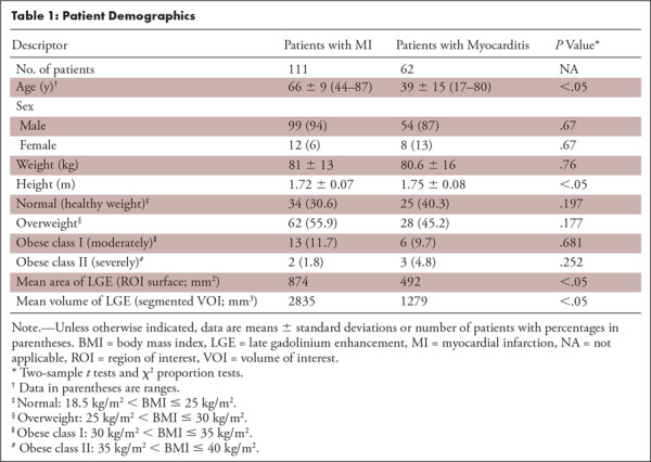
Among these 173 patients, 111 (64%) patients (12 women; mean age, 66 years ± 9 [standard deviation]) had MI, whereas the myocarditis group included 62 (36%, 62 of 173) patients (eight women; mean age, 39 years ± 15; see Table 1).

MRI Examinations

Of the 173 examinations, 162 were performed with a 1.5-T scanner (Achieva; Philips Healthcare, Best, the Netherlands) and 11 were performed with a 3-T scanner (MAGNETOM Skyra; Siemens Healthcare, Erlangen, Germany). For signal reception, five-element and 18-element phased-array receiver coils were used, respectively. First, cine images of the heart were acquired in four standard geometries (ie, short-axis, two-chamber, three-chamber, and four-chamber views) by using a balanced steady-state free precession sequence with breath-hold technique and retrospective electrocardiographic triggering. T2-weighted images were acquired by using a double-inversion black-blood spin-echo sequence in three short-axis slices. For the depiction of myocardial scar or fibrosis, LGE images in three short-axis slices were acquired 10–15 minutes after administration of a bolus of 0.2 mmol of gadobutrol per kilogram of body weight (Gadovist; Bayer Schering, Berlin, Germany). A 3D inversion recovery gradient-echo MRI sequence (at 1.5 T) and 2D phase-sensitive inversion recovery sequence (at 3 T) were used.

As texture features can be affected by image resolution (12), all 512 × 512 matrix images were resampled through a one-dimensional (1D) nearest-neighbor interpolation to achieve a uniform pixel size of 0.65 × 0.65 mm² (1.54 pixels per millimeter). We resampled on the XY plane and not in the z-axis to preserve in-plane information. This was done because the XY plane was considered richer in information and was easier to assess, whereas the information out-of-plane is intrinsically poorer owing to strongly anisotropic MRI acquisition.

Subjective Visual Analysis

LGE images were subjectively analyzed for the differentiation between MI and myocarditis by two blinded and independent readers (reader 1 [E.G.], in the 1st year of experience in cardiovascular imaging, and reader 2 [M.M.], having 5 years of experience). For the 2D subjective visual analysis, reader 1 and reader 2 were presented one short-axis LGE image per patient showing the largest extent of LGE. For the 3D subjective visual analysis, the same two readers were presented all short-axis images showing LGE in each patient. To avoid recall bias, the readout on 3D images was performed 3 months after the 2D readout.

Images were presented at fixed window settings, but readers were allowed to change the settings according to individual preferences. All readers were blinded to patient information, results from the other readers and all other imaging tests, and final diagnosis.

Machine Learning–based Radiomics Analysis

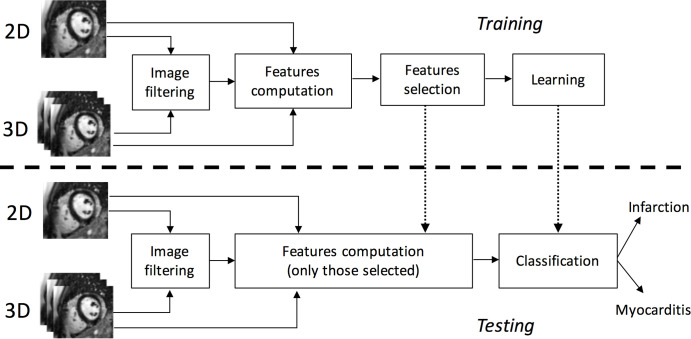
The analysis aimed to yield a set of 2D or 3D features, either from the original or from filtered images. Feature evaluation and feature selection on a disjoint validation set permits the build of the learning model, which is finally trained. To perform the classification on a new set of MR images (test patients), the system exploits both the best feature set and the trained model defined in the previous stage (Fig 1).

Figure 1:

Schematic illustration of the radiomics and machine learning approach. 3D = three dimensional, 2D = two dimensional.

Filtering and Feature Computation

In the 2D analysis, a region of interest (ROI) was selected for segmentation and feature extraction. The slice showing the largest extent of LGE used for subjective visual analysis was chosen (described previously in this article). To compute the 3D descriptors, all MR image slices enclosing the LGE lesion were segmented, creating a 3D volume of interest (VOI). The selection of the slices and the manual segmentation of ROIs and VOIs were performed by one expert reader (reader 3 [J.v.S.], with 5 years of experience in cardiovascular imaging). For slice selection, a proprietary viewing station (Impax; Agfa HealthCare, Mortsel, Belgium) and a clinically used viewer (Syngo.Via; Siemens Healthineers, Forchheim, Germany) were used, while the manual segmentation of ROIs and VOIs was performed with open-source software (3DSlicer; Brigham and Women’s Hospital, Boston, Mass). Figures 2 and 3 provide representative examples.

Figure 2a:

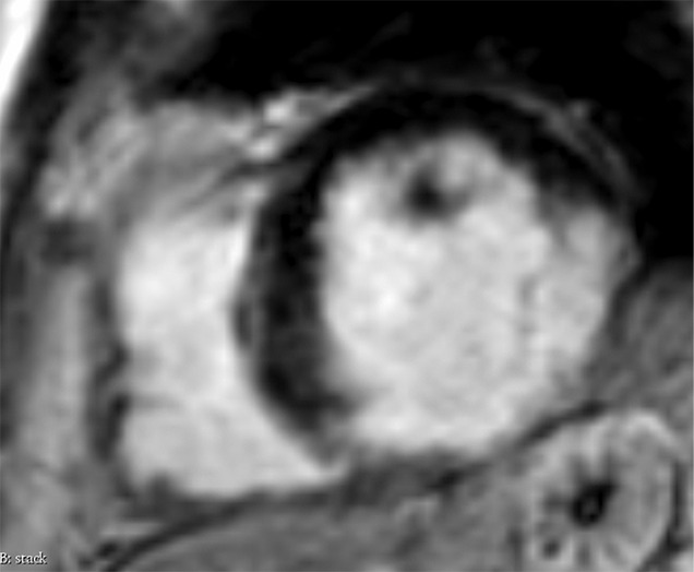
Images in a 74-year-old male patient with subacute myocardial infarction. (a) Late gadolinium enhancement cardiac MR image in the short-axis view. (b) Two-dimensional region-of-interest segmentation of the infarcted area. (c) Three-dimensional volume-of-interest segmentation of the infarcted area.

Figure 3a:

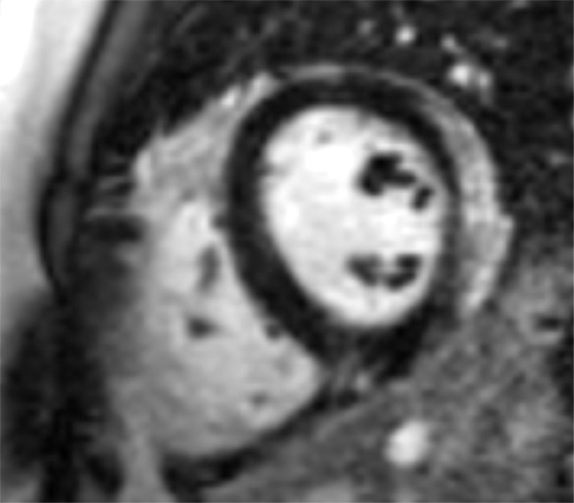
Images in a 24-year-old male patient with acute myocarditis. (a) Late gadolinium enhancement (LGE) cardiac MR image in the short-axis view. (b) Two-dimensional region-of-interest segmentation of the LGE area. (c) Three-dimensional volume-of-interest segmentation of the LGE area.

Figure 2b:

Images in a 74-year-old male patient with subacute myocardial infarction. (a) Late gadolinium enhancement cardiac MR image in the short-axis view. (b) Two-dimensional region-of-interest segmentation of the infarcted area. (c) Three-dimensional volume-of-interest segmentation of the infarcted area.

Figure 2c:

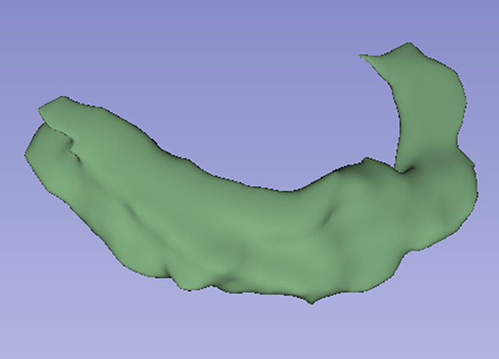
Images in a 74-year-old male patient with subacute myocardial infarction. (a) Late gadolinium enhancement cardiac MR image in the short-axis view. (b) Two-dimensional region-of-interest segmentation of the infarcted area. (c) Three-dimensional volume-of-interest segmentation of the infarcted area.

Figure 3b:

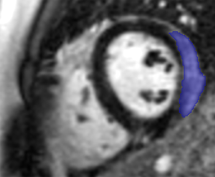
Images in a 24-year-old male patient with acute myocarditis. (a) Late gadolinium enhancement (LGE) cardiac MR image in the short-axis view. (b) Two-dimensional region-of-interest segmentation of the LGE area. (c) Three-dimensional volume-of-interest segmentation of the LGE area.

Figure 3c:

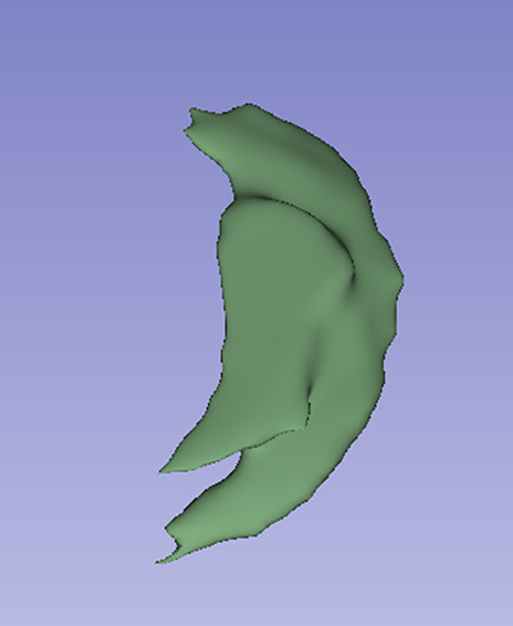
Images in a 24-year-old male patient with acute myocarditis. (a) Late gadolinium enhancement (LGE) cardiac MR image in the short-axis view. (b) Two-dimensional region-of-interest segmentation of the LGE area. (c) Three-dimensional volume-of-interest segmentation of the LGE area.

We computed features from original images, wavelet-filtered subband images, and exponential-filtered images, as image preprocessing through various filters has proven to be effective in pattern recognition applications (13). It is worth noting that preprocessing the images through a filter bank is not a mandatory step and, to the best of our knowledge, there exists no standard of reference yet that clearly demonstrates how compulsory and/or advantageous the use of a filter bank is: Indeed, some authors perform it (14,15) and others do not (16). Computation of features from both the original and filtered images provides a larger and possibly richer set of descriptors processed by the feature selection algorithm.

In case of the first filter, for original images we applied the stationary wavelet transform filter, which aims at removing noise, highlighting the edges, and enhancing image resolution (17). As filtering parameters, we set a “coif1” wavelet and one level of wavelet decomposition. This provided four and eight wavelet subband images for 2D and 3D images, denoted as LL (low-low), LH (low-high), HL (high-low), HH (high-high) and LLL, LLH, LHL, LHH, HLL, HLH, HHL, HHH, respectively. For example, in the 2D case, the LL image obtained was the original image filtered by a low-pass filter along the rows and then along the corresponding columns. This image represents an approximation of the original one. Conversely, HL and LH were obtained by sequentially applying low- and high-pass decomposition filters along image rows and then along image columns. These two images mostly contain horizontal and vertical edges, respectively. Finally, the HH image can be considered as a block holding information about the edges of the original image along diagonal directions. The extension to the 3D case considers the third dimension as the “depth” of the image stack.

The exponential filter was selected as second filter for smoothing the original image while preserving edges (18). The filtering function applied was as follows:

where 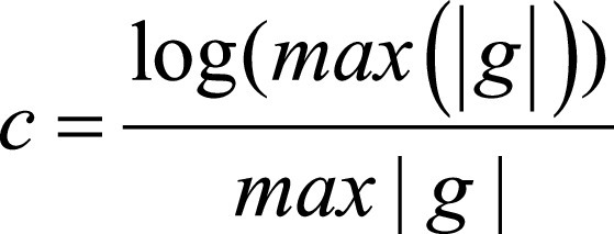and g is the original gray-level pixel intensity at coordinates (x, y). The use of an exponential filter rescales the gray-level values on the range of the initial image.

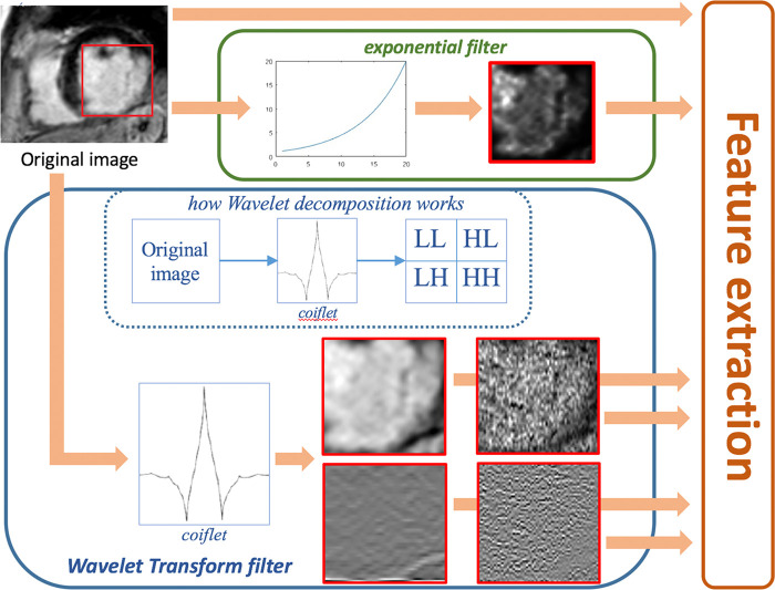
A visual example of the 2D filtering process is illustrated in Figure 4: First, the ROI is cropped from the original image; then the cropped image is filtered into the wavelet subbands (LL, LH, HL, HH) and with the exponential operator. The wavelet subband images can be thought of as images obtained through sequential high- and low-pass filters along the original image rows and columns, alternatively. The features are then computed from every cropped image (original and filtered ones).

Figure 4:

Graphical representation of the two-dimensional filtering process (preferred to three-dimensional filtering for simplicity of visualization). Features were computed from original images, from four wavelet-filtered sub-band images and from exponential-filtered images. In the red boxes within each filter, the results of the filters applied to the red box in the original image are shown. The dotted blue box summarizes how wavelet filtering decomposes the original image.

The selected features were divided into groups and were computed by using PyRadiomics, an open-source software platform (19), which enables following and comparing results (20). For each of the seven groups computed, we subsequently provide a short description. More detailed definitions can be found in the PyRadiomics documentation (https://pyradiomics.readthedocs.io/en/latest/index.html) and in Appendix E1 (supplement).

First-order statistics describe the distribution of gray-level intensities within the ROI or VOI by common metrics such as entropy, energy, and statistical moments up to the fourth order of the first-order image histogram.

Shape-based measures represent the size or shape of the ROI or VOI, such as the volume, surface area, sphericity, and maximum diameter either in 2D or 3D.

Gray-level co-occurrence matrix represents the distribution of co-occurring values between neighboring pixels according to different displacements (21).

Gray-level run length matrix (22) measures gray-level runs that are defined as the length in the number of consecutive pixels that have the same gray-level value.

Gray-level size zone matrix (23) quantifies the gray-level zones in an image.

Neighboring gray tone difference matrix (24) quantifies the differences between a gray value and the average gray value of its neighbors within a certain distance.

Gray-level dependence matrix (25) describes the gray-level dependencies in an image.

Except from the shape-based features, which are independent of intensity values, all other descriptors were computed both for the original 2D image and for the five filtered images, yielding a total of 563 and 933 features for 2D and 3D analyses, respectively.

In addition, we assessed the influence of the resampling step on the results. Therefore, besides the 1D nearest-neighbor interpolation, we extracted the same 2D and 3D features both from spline-interpolated images and from the original MR images without resampling.

Feature Selection

As reported previously, a feature vector “x” composed of hundreds of elements was available for each patient. However, it is known that a limited yet salient feature set simplifies both the pattern representation and the classifiers that are built on the selected representation, as it alleviates the curse of dimensionality. In addition, feature selection is essential in every machine learning pipeline to simplify the model (make it easier to interpret), speed up training time, and enhance generalization by reducing overfitting. This usually happens because data contain many features that are either redundant, irrelevant, or noisy and can thus be removed without incurring much loss of information.

To this aim, the recursive feature elimination (RFE) method was used. RFE is a supervised feature-ranking criterion that sorts the input features from the most to the least discriminating ones, retains only a relevant subset of descriptors, and has proven to be effective to avoid overfitting (26). The feature selection step was performed in the internal cross-validation (CV) loop, as detailed in the next section when presenting the experimental evaluation. With reference to the total number of features to be retained, we followed the approach proposed by Hua et al (27), who suggested that when feature correlation is high, the optimal feature size is proportional to , where N is the sample size: accordingly, we retained the 13 () most discriminating features. This procedure was applied for each fold in the training phase of the nested CV (see Fig 1). In the test phase, we computed the retained descriptors that were then given as input to the trained classifier.

A further test aimed at evaluating the impact of the feature selection step within the pipeline. Hence, besides RFE, all experiments were run by using principal component analysis (PCA), which is an unsupervised and nonparametric method for extracting relevant information from data sets. This was applied in the internal CV loop, and the number of retained components was set considering their explained variance, making use of the scree plot (28). Using this plot, and also according to common practice in machine learning (28), we retained the PCA components mapping 99% of data variability, which correspond to 60 and 80 PCA components for 2D and 3D features, respectively.

Classifiers

Fernández-Delgado et al (29) suggested that it would be preferable to adopt classifiers belonging to different classifier families. Accordingly, we included linear discriminant analysis (LDA) as a statistical classifier, k-nearest neighbor (k-NN) as a distance-based classifier, multilayer perceptron as a neural network, support vector machine (SVM) as a kernel machine, and TreeBagger (TB) as an ensemble of trees. Apart from LDA, which has no hyperparameters to tune, the following hyperparameters were validated in the internal CV loop as follows: for k-NN, the number of neighbors was searched within the set {1,3,5}; for multilayer perceptron, one hidden layer was set, and the number of neurons in that hidden layer was tuned as a hyperparameter in the internal CV. The rule of thumb proposed by Heaton (30) was adopted for selecting the maximum number of hidden neurons: namely, the number of hidden neurons should be two-third the size of the input layer plus the size of the output layer. Thus, the number of hidden neurons was varied from 86 (almost half the size of the input layer) to 117, with unitary step. For SVM, we explored different kernel functions, namely linear, radial basis, and polynomial, which were the hyperparameters to be tuned (while using default values of specific kernel hyperparameters). Finally, for TB, the number of trees in the ensemble was varied within the interval [5, 30], with a step of 5. All other parameters were set to their default values.

We tuned one hyperparameter per classifier for two main reasons: first, the no free lunch theorems for optimization (31) indicate that it is impossible to tune an algorithm such that it will have optimal settings for any possible problem and second, in many cases, the tuning of many parameters cannot significantly outperform the default values of a classifier suggested in the literature (32). Therefore, the default parameters suggested by the machine learning libraries, which correspond to those in the literature, should not be considered inappropriate; and it is reasonable that the classifier that wins on average in all experiments would also outperform the others if a better setting was considered (33).

Experimental Evaluation

All experiments were carried out by applying nested CV, which implies that external and internal CVs were performed. In a “standard” CV, the test set is used to both select the values of the hyperparameters and evaluate the model risks to optimistically bias model performances (34). Nested CV overcomes this issue: first, an outer CV splits the patients into external training and test sets. Second, an inner CV resplits the external training patients into internal training and validation sets where the latter is used to tune the hyperparameters of the classifiers (select the best model) and to select the features. Finally, the tuned model was evaluated with the left-out test fold. To avoid bias in performance evaluation, nested CV was run in stratified mode, that is, preserving the a priori class distribution among CV folds. We set the number of folds to 10 both for the internal and external CVs. This implies that the 173 patients were first divided into 10 equal-sized groups: nine constitute the external training set (corresponding to 156 patients) and one composed of 17 patients makes up the external test set. Subsequently, in the inner CV, the 156 patients belonging to the external training set were further divided into 10 equal-sized groups, so that nine groups composed of 140 patients made up the internal training set and one containing 16 patients served as the validation set. First, the validation set changed for each of the internal folds, and the classifier tuned its hyperparameters. Then, the trained classifier was evaluated on the 17 test patients. Third, the test set fold changed and the tuning started all over again. This routine went on iteratively until all the 10 test folds were changed. Finally, results of the test folds were averaged. Furthermore, to reduce the bias introduced by the random choice of patients at each CV split, the whole procedure was run 10 times (10 random realizations), and the results were averaged out. Given the size of our data set, the nested CV was explicitly applied to assess how the results of each classifier would generalize to an independent data set, also having the advantage of finding an optimal tradeoff between bias and variance of the model (35).

Statistical Analysis

In this study, sensitivity represents the proportion of patients with MI who were correctly identified, specificity represents the fraction of patients with myocarditis who were correctly identified, and precision (or positive predictive value) represents the fraction of patients with MI with regard to all subjects classified as patients with MI by the classifier. Accuracy corresponds to the total number of patients correctly classified, regardless of the class. The subjective visual analysis was calculated by using the same descriptors mentioned above for both readers separately.

To statistically compare the classification results of the five classifiers, several nonparametric Wilcoxon signed-rank tests were performed (36). More specifically, over the 10 random realizations, we decided to maintain the same patient order split (inner and outer CV) such that, for every realization, every classifier was validated and tested with the same patients. By doing this, the per-patient proportion of correctly/incorrectly classified patients was preserved among the five algorithms. For simplicity, the Wilcoxon signed-rank tests that we performed only accounted for the accuracy of the classifiers. This seems a reasonable hypothesis, as there were no cases where the accuracy untruthfully reflected the other parameters’ trend. In summary, we performed several Wilcoxon signed-rank tests to compare the accuracy values of the five classifiers over the 10 random realizations: the goal of the tests was to verify the null hypothesis that these per-patient samples came from the same distribution. For the Wilcoxon tests, we used a threshold level α =.05 for comparing P values and adjusted α with Bonferroni correction when performing multiple comparisons ().

Results

Subjective Visual Image Analysis

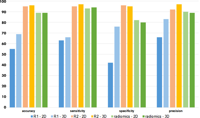
Subjective visual analysis for differentiating MI and myocarditis based on LGE images showed variable performances between 2D and 3D images and between readers. For the 2D readout, higher accuracy (95%), sensitivity (95%), specificity (96%), and precision (92%) were found for the more experienced reader (reader 2) as compared with those found for the less-experienced reader (reader 1; 55%, 63%, 42%, and 66%, respectively). For the 3D readout, the performance values were 96%, 97%, 95%, and 97% for reader 2 and 69%, 66%, 76%, and 83% for reader 1, respectively (Fig 5).

Figure 5:

Bar charts show the accuracy, sensitivity, specificity, and precision (in percentages) of the two readers, reader 1 and reader 2, performing a subjective visual analysis of late gadolinium enhancement images and of the radiomics approach with both two-dimensional (2D) and three-dimensional (3D) image data. For the radiomics approach, 2D-derived support vector machine trained with recursive feature elimination and 3D-derived linear discriminant analysis trained with principal component analysis are shown.

Radiomics Approach

For the 2D features, the RFE feature selector led to the highest performances, whereas for the 3D features, the PCA was the best-performing feature selector. The results obtained using the 2D features and RFE feature selection are reported in Table 2; results obtained using the 3D features and PCA feature selection are listed in Table 3.

Table 2:

Classification Results with Two-dimensional Features Extracted with Recursive Feature Elimination and One-dimensional Nearest-Neighbor Interpolation

Table 3:

Classification Results with Three-dimensional Features Extracted with Principal Component Analysis and One-dimensional Nearest-Neighbor Interpolation

It can be seen that for the 2D analysis, the SVM algorithm reached the highest overall performances (accuracy 88%, sensitivity 92%, specificity 81%, and precision 90%), whereas for the 3D analysis, the LDA was the best classifier (accuracy 89%, sensitivity 94%, specificity 79%, and precision 89%; see Fig 5). Most of the experiments showed low standard deviations, suggesting that the results were not substantially affected by the specific fold under test.

The performance of the radiomics approach was higher than that of the less-experienced reader (reader 1) and slightly lower than that of the experienced reader (reader 2) performing a subjective visual analysis of both 2D and 3D data.

We investigated the performance of the five algorithms on the subset of patients misclassified by the less-experienced reader: The LDA model reached a 93% accuracy, 95% sensitivity, 86% specificity, and 94% precision.

In addition, we created a subset comprising patients with transmural LGE. Here, we included 64 patients (56 with MI and eight with myocarditis). Given this small portion of patients with myocarditis, we ran a fourfold CV yielding that none of the algorithms reached a specificity higher than 60%.

For the 2D-RFE measures, we compared the best classifier SVM with the other four classifiers (SVM vs k-NN, SVM vs LDA, SVM vs multilayer perceptron, and SVM vs TB) through Wilcoxon signed-rank tests. For the 3D PCA-derived descriptors, we compared the LDA with the other four algorithms (LDA vs k-NN, LDA vs multilayer perceptron, LDA vs SVM, and LDA vs TB). The results of the comparisons among the classifiers fed with 2D and 3D descriptors are provided in Table 4. As we tested the same best algorithm against the other four, for Table 4, we adjusted the threshold α with Bonferroni correction (ie, ). Although for the 2D features the null hypothesis could not be rejected, for the 3D features, the LDA yielded significantly higher results than the other four classifiers (all P <.0125).

Table 4:

Results of the Wilcoxon Signed-Rank Tests for Comparison among Classifiers

In addition, we compared predictions of each classifier trained using 2D and 3D features (ie, 2D-SVM vs 3D-SVM and 2D-TB vs 3D-TB) with RFE. Here, we found significant differences for all the five classifiers (P <.05, each). In particular, as classification performances were always higher in the 2D analysis, we can infer that 2D features statistically hold more information than 3D features when training with RFE.

Effect of Image Resampling

We tested the impact of image resampling on classification results. As the same best algorithm obtained with 1D nearest-neighbor resampling was compared with the corresponding best models achieved first with spline resampling and then without resampling, for these two tests, we corrected α to 0.025 (ie, ). Regarding the experiments run with spline interpolation, the 2D-derived LDA was the algorithm that outperformed the others, with accuracy, sensitivity, specificity, and precision equaling 84%, 92%, 69%, and 84%, respectively. These classification performances were inferior to those achieved with the 1D nearest-neighbor resampling (P <.025 when comparing the best classifier trained on spline-interpolated images and the best one trained on 1D nearest-neighbor interpolated images).

Results without image resampling were not significantly different from those obtained with 1D nearest-neighbor resampling: the 2D-derived LDA trained with nonresampled images had an accuracy of 87%, being not significantly different from the 2D-derived SVM trained with 1D nearest-neighbor resampled images (88%; P = .10).

Effect of Feature Selection

When training with PCA, the LDA classifier showed the highest performances for both 2D and 3D features (accuracy, sensitivity, specificity, and precision: 86%, 93%, 75%, and 87% [2D] and 89%, 94%, 79%, and 89% [3D], respectively). To assess the impact of feature resampling in 2D, we compared the best classifier-obtained training with RFE (SVM) and the best classifier-obtained training with PCA (LDA). In the 3D analysis, we compared the best two classifiers obtained with the two feature selection techniques (3D-RFE-LDA and 3D-PCA-LDA): Whereas in 2D, PCA worsened performances, 3D features extracted with PCA led to improved performances (both, P <.05).

Regarding the feature selection of 2D descriptors with RFE, the original and wavelet-filtered images held most information, even if some features coming from the exponential-filtered images were also included. More specifically, the feature groups that contained the most discriminating features were gray-level run length matrix, gray-level dependence matrix, and gray-level size zone matrix.

Similarly, for the feature selection of 3D descriptors with RFE, the original and wavelet-filtered images yielded the majority of relevant features. Only for images resampled with 1D nearest neighbor, the exponential-small area emphasis feature was also included. With 3D images, the groups that contained the most discriminating features were gray-level size zone matrix, gray-level dependence matrix, and shape.

We performed further simulations excluding feature groups: for instance, we trained the classifiers only with the wavelet- and exponential-derived features (without the originals), only with the original- and wavelet-derived features (without the exponentials), or only with the original- and exponential-derived features (without the wavelets). These three configurations led to an average accuracy decrease (among the five classifiers) of 4%, 4%, and 4%, respectively, with 2D descriptors. Similarly, they led to an average accuracy decrease (among the five classifiers) of 4%, 1%, and 3%, respectively, with 3D descriptors. These findings suggest that among the entire subset of features created by the feature selector, there are always features coming from the three groups (original features, wavelet-derived features, and exponential-derived features).

More detailed insight of the feature selection with RFE is shown in Tables E1 and E2 (supplement) where the five most recurrent selected features are shown for each experiment. The descriptors coming from unsupervised feature selection were not reported because the PCA intrinsically modifies the feature space identifying the components that better explain the variability of the data. Hence, the original information of the features is lost, and the obtained descriptors are not comparable with those selected by RFE.

Discussion

This study sought to investigate whether a radiomics approach might enable the differentiation of LGE on cardiac MR images as originating from MI or myocarditis. Our results attained using 2D features and RFE feature selection showed that the SVM classifier yielded the highest accuracy for this differentiation, although no significant differences were found while comparing the SVM performance with those obtained with the other machine learning algorithms. This finding suggests that, as a whole, the five 2D classifiers were equally accurate and robust with regard to this binary task. The robustness is further proven by the low variance of the scoring parameters. When the classifiers were trained with 3D descriptors, instead, the highest performances were attained using PCA feature selection. In particular, the LDA proved to be the most accurate algorithm, thereby outperforming the other four. Interestingly, the radiomics approach showed higher performance on both 2D and 3D data than that of an unexperienced reader performing visual subjective analysis, while the reader with more experience in cardiovascular imaging had a slightly higher overall performance than the radiomics approach.

To our knowledge, no study so far has investigated the accuracy of both 2D and 3D descriptors in cardiac imaging. Our analyses assessing the diagnostic performance of volumetric descriptors compared with the planar ones indicated that, with RFE, 2D held more information than 3D descriptors, leading to higher classification performances. This could be possibly related to the inherent nonisotropic spatial resolution of MRI. We thus suggest that 2D features be preferred for the task at hand, also because they are faster to extract than 3D features.

We also explored how the feature selection step affected classification performances. Thus, the same experiments were performed replacing RFE with PCA. While with 2D features, the use of PCA reduced performances, with 3D features it instead increased classification results. This indicates that, with 2D descriptors, the prior knowledge of the class labels (MI or myocarditis) helps in creating a more discriminating feature set. Conversely, this reasoning does not hold for 3D descriptors where the data set holds enough information that is innately sufficient to separate the relevant sample descriptors and the prior knowledge of the class labels is therefore unnecessary.

To assess the impact of the resampling step, spline resampling was tested in addition to the 1D nearest neighbor. Resampling is usually applied to get a uniform pixel size because texture features might be affected by image resolution (12). In our study, the image resolution varied because two different MR scanners with corresponding protocols were used. Moreover, images generated by the same scanner had different in-plane resolutions. Using the spline resampling, the 2D-derived LDA algorithm attained best performances with an accuracy of 84%, but classification scores were lower than those attained with the 1D nearest-neighbor SVM. When using no resampling, instead, performance results did not vary statistically from those obtained with 1D nearest-neighbor resampled images. As suggested by Larue et al (37), image resampling is usually recommended, especially when working with images acquired from different scanners, to improve consistency and reproducibility of feature sets. In our work, only a small percentage (6%) of the images were from one MR scanner, and conducting the analysis without any resampling led similarly to robust and accurate results. However, we did not conduct a detailed comparison between the different feature sets as in a previous study (37), as this was beyond the scope of this study.

Comparing radiomics with human readers, we found that the performance of radiomics was higher than that from subjective visual analysis of a reader with little experience, whereas the advanced reader performed better, overall. This was true for both 2D and 3D image data. Subanalyses revealed that radiomics performed accurately in patients misclassified by the less-experienced reader, whereas it had limited accuracy when both MI and myocarditis had a transmural pattern of LGE. Certainly, further research is warranted on this topic including larger data sets that might open the way for deep learning with potentially even higher performance levels. Another direction of research could include semiautomatic or automatic segmentation techniques for defining ROIs and VOIs. Moreover, the application of other filters besides wavelet and exponential filters is another interesting topic worth investigating, and their use would yield numerous feature sets and possibly higher classification performances. Similarly, the application of different wavelets beyond “coif1” for the stationary wavelet transform could have yielded a different feature set. A potential clinical application of the radiomics approach, when achieving a sufficiently high diagnostic performance, could be that of a computer-aided diagnosis system supporting radiologists in reading cardiac MRI cases.

The following study limitations have to be acknowledged. First, we included a limited sample size in this study, and the availability of a larger data set could permit not only studying how much the use of different MR scanners affects the results but also investigating methods to harmonize images acquired with various devices. Second, the prior probabilities of the two classes (MI and myocarditis) of our patient population do not accurately reflect the natural prevalence of the diseases (38,39). Third, segmentations were performed by one single reader and not by using semiautomated or automated techniques, the latter being more reproducible than manual segmentations. Fourth, this study did not include T2-weighted, early gadolinium-enhanced T1-weighted, or T1 and T2 mapping information into the analyses. Including those features and image information might have further improved the performance of the machine learning algorithms. Fifth, we did not include patients with other cardiac diseases being associated with LGE, such as hypertrophic obstructive cardiomyopathy. Expanding the list of possible differential diagnoses for LGE could have reduced the accuracy of the proposed algorithm. Sixth, inherent shortcomings of MRI include nonisotropic voxel sizes because of the limited through-plane resolution. Resampling images to be isotropic would have led to a drastic loss of in-plane information. Finally, it is possible that too many easy cases were included in our analyses, and performing an analysis in a subset of patients showing challenging imaging findings only could have affected the performances of both the machine and human readers.

In conclusion, our study indicated that radiomics features, identified through machine learning, enabled distinguishing MI from myocarditis based on LGE at MRI with high accuracy.

References

- 1.Mewton N, Liu CY, Croisille P, Bluemke D, Lima JA. Assessment of myocardial fibrosis with cardiovascular magnetic resonance. J Am Coll Cardiol 2011;57(8):891–903. [DOI] [PMC free article] [PubMed] [Google Scholar]
- 2.van der Wall EE, Vliegen HW, de Roos A, Bruschke AV. Magnetic resonance imaging in coronary artery disease. Circulation 1995;92(9):2723–2739. [DOI] [PubMed] [Google Scholar]
- 3.Berg J, Kottwitz J, Baltensperger N, et al. Cardiac magnetic resonance imaging in myocarditis reveals persistent disease activity despite normalization of cardiac enzymes and inflammatory parameters at 3-month follow-up. Circ Heart Fail 2017;10(11):e004262. [DOI] [PubMed] [Google Scholar]
- 4.Patriki D, Gresser E, Manka R, Emmert MY, Lüscher TF, Heidecker B. Approximation of the incidence of myocarditis by systematic screening with cardiac magnetic resonance imaging. JACC Heart Fail 2018;6(7):573–579. [DOI] [PubMed] [Google Scholar]
- 5.Baessler B, Luecke C, Lurz J, et al. Cardiac MRI texture analysis of T1 and T2 maps in patients with infarctlike acute myocarditis. Radiology 2018;289(2):357–365. [DOI] [PubMed] [Google Scholar]
- 6.Larroza A, López-Lereu MP, Monmeneu JV, et al. Texture analysis of cardiac cine magnetic resonance imaging to detect nonviable segments in patients with chronic myocardial infarction. Med Phys 2018;45(4):1471–1480. [DOI] [PubMed] [Google Scholar]
- 7.Antunes S, Esposito A, Palmisanov A, Colantoni C, de Cobelli F, Del Maschio A. Characterization of normal and scarred myocardium based on texture analysis of cardiac computed tomography images. Engineering in Medicine and Biology Society (EMBC), 2016 IEEE 38th Annual International Conference, 2016; 4161–4164. [DOI] [PubMed]
- 8.Baessler B, Mannil M, Oebel S, Maintz D, Alkadhi H, Manka R. Subacute and chronic left ventricular myocardial scar: accuracy of texture analysis on nonenhanced cine MR images. Radiology 2018;286(1):103–112. [DOI] [PubMed] [Google Scholar]
- 9.Kotu LP, Engan K, Borhani R, et al. Cardiac magnetic resonance image-based classification of the risk of arrhythmias in post-myocardial infarction patients. Artif Intell Med 2015;64(3):205–215. [DOI] [PubMed] [Google Scholar]
- 10.Ambale-Venkatesh B, Yang X, Wu CO, et al. Cardiovascular event prediction by machine learning: the Multi-Ethnic Study of Atherosclerosis. Circ Res 2017;121(9):1092–1101. [DOI] [PMC free article] [PubMed] [Google Scholar]
- 11.Friedrich MG, Sechtem U, Schulz-Menger J, et al. Cardiovascular magnetic resonance in myocarditis: a JACC white paper. J Am Coll Cardiol 2009;53(17):1475–1487. [DOI] [PMC free article] [PubMed] [Google Scholar]
- 12.Leijenaar RT, Nalbantov G, Carvalho S, et al. The effect of SUV discretization in quantitative FDG-PET Radiomics: the need for standardized methodology in tumor texture analysis. Sci Rep 2015;5(1):11075. [DOI] [PMC free article] [PubMed] [Google Scholar]
- 13.Sopharak A, Dailey MN, Uyyanonvara B, et al. Machine learning approach to automatic exudate detection in retinal images from diabetic patients. J Mod Opt 2010;57(2):124–135. [Google Scholar]
- 14.Nazeri A, Crandall J, Laforest R, Wahl R. The impact of volume of interest size on 18F-FDG PET radiomic feature robustness: a phantom study. J Nucl Med 2018;59(supplement 1):1752. [Google Scholar]
- 15.Depeursinge A, Fageot J, Andrearczyk V, Ward JP, Unser M. Rotation invariance and directional sensitivity: spherical harmonics versus radiomics features. International Workshop on Machine Learning in Medical Imaging. Cham, Switzerland: Springer, 2018. [Google Scholar]
- 16.Bai W, Shi W, Ledig C, Rueckert D. Multi-atlas segmentation with augmented features for cardiac MR images. Med Image Anal 2015;19(1):98–109. [DOI] [PubMed] [Google Scholar]
- 17.Demirel H, Anbarjafari G. IMAGE resolution enhancement by using discrete and stationary wavelet decomposition. IEEE Trans Image Process 2011;20(5):1458–1460. [DOI] [PubMed] [Google Scholar]
- 18.Basu M, Su M. Image smoothing with exponential functions. Intern J Pattern Recognit Artif Intell 2001;15(4):735–752. [Google Scholar]
- 19.van Griethuysen JJM, Fedorov A, Parmar C, et al. Computational radiomics system to decode the radiographic phenotype. Cancer Res 2017;77(21):e104–e107. [DOI] [PMC free article] [PubMed] [Google Scholar]
- 20.Yip SS, Aerts HJ. Applications and limitations of radiomics. Phys Med Biol 2016;61(13):R150–R166. [DOI] [PMC free article] [PubMed] [Google Scholar]
- 21.Haralick RM, Shanmugam K, Dinstein IH. Textural features for image classification. IEEE Trans Syst Man Cybern 1973;SMC-3(6):610–621. [Google Scholar]
- 22.Galloway MM. Texture analysis using grey level run lengths. NASA STI/Recon Technical Report N. 75. July 1974.
- 23.Thibault G, Fertil B, Navarro C, et al. Shape and texture indexes application to cell nuclei classification. Intern J Pattern Recognit Artif Intell 2013;27(1):1357002. [Google Scholar]
- 24.Amadasun M, King R. Textural features corresponding to textural properties. IEEE Trans Syst Man Cybern 1989;19(5):1264–1274. [Google Scholar]
- 25.Zwanenburg A, Leger S, Vallières M, Löck S. Image biomarker standardisation initiative. arXiv:1612.07003. [preprint] https://arxiv.org/abs/1612.07003. Posted December 21, 2016. Accessed July 2018.
- 26.Guyon I, Weston J, Barnhill S, Vapnik V. Gene selection for cancer classification using support vector machines. Mach Learn 2002;46(1-3):389–422. [Google Scholar]
- 27.Hua J, Xiong Z, Lowey J, Suh E, Dougherty ER. Optimal number of features as a function of sample size for various classification rules. Bioinformatics 2005;21(8):1509–1515. [DOI] [PubMed] [Google Scholar]
- 28.Cattell RB. The scree test for the number of factors. Multivariate Behav Res 1966;1(2):245–276. [DOI] [PubMed] [Google Scholar]
- 29.Fernández-Delgado M, Cernadas E, Barro S, Amorim D. Do we need hundreds of classifiers to solve real world classification problems? J Mach Learn Res 2014;15(1):3133–3181. [Google Scholar]
- 30.Heaton J. Introduction to neural networks with Java. Washington University, St Louis, Mo: Heaton Research, 2008. [Google Scholar]
- 31.Wolpert DH, Macready WG. No free lunch theorems for optimization. IEEE Trans Evol Comput 1997;1(1):67–82. [Google Scholar]
- 32.Arcuri A, Fraser G. Parameter tuning or default values? An empirical investigation in search-based software engineering. Empir Softw Eng 2013;18(3):594–623. [Google Scholar]
- 33.Fernández A, López V, Galar M, del Jesus MJ, Herrera F. Analysing the classification of imbalanced data-sets with multiple classes: binarization techniques and ad-hoc approaches. Knowl Base Syst 2013;42:97–110. [Google Scholar]
- 34.Cawley GC, Talbot NL. On over-fitting in model selection and subsequent selection bias in performance evaluation. J Mach Learn Res 2010;11:2079–2107. [Google Scholar]
- 35.Kohavi R. A study of cross-validation and bootstrap for accuracy estimation and model selection. IJCAI’95 Proceedings of the 14th International Joint Conference on Artificial Intelligence–Vol 2, Montreal, Quebec, Canada, August 20–25, 1995. San Francisco, Calif: Morgan Kaufmann, 1995; 1137–1143.
- 36.Wilcoxon F. Individual comparisons by ranking methods. Biom Bull 1945;1(6):80–83. [Google Scholar]
- 37.Larue RTHM, van Timmeren JE, de Jong EEC, et al. Influence of gray level discretization on radiomic feature stability for different CT scanners, tube currents and slice thicknesses: a comprehensive phantom study. Acta Oncol 2017;56(11):1544–1553. [DOI] [PubMed] [Google Scholar]
- 38.Fung G, Luo H, Qiu Y, Yang D, McManus B. Myocarditis. Circ Res 2016;118(3):496–514. [DOI] [PubMed] [Google Scholar]
- 39.Roger VL. Epidemiology of myocardial infarction. Med Clin North Am 2007;91(4):537–552, ix. [DOI] [PMC free article] [PubMed] [Google Scholar]
Associated Data
This section collects any data citations, data availability statements, or supplementary materials included in this article.