Investigation of Low-Dose CT Image Denoising Using Unpaired Deep Learning Methods

Abstract

Low-dose computed tomography (LDCT) is desired due to prevalence and ionizing radiation of CT, but suffers elevated noise. To improve LDCT image quality, an image-domain denoising method based on cycle-consistent generative adversarial network (“CycleGAN”) is developed and compared with two other variants, IdentityGAN and GAN-CIRCLE. Different from supervised deep learning methods, these unpaired methods can effectively learn image translation from the low-dose domain to the full-dose (FD) domain without the need of aligning FDCT and LDCT images. The results on real and synthetic patient CT data show that these methods can achieve peak signal-to-noise ratio (PSNR) and structural similarity index (SSIM) comparable to, if not better than, the other state-of-the-art denoising methods. Among CycleGAN, IdentityGAN, and GAN-CIRCLE, the later achieves the best denoising performance with the shortest computation time. Subsequently, GAN-CIRCLE is used to demonstrate that the increasing number of training patches and of training patients can improve denoising performance. Finally, two non-overlapping experiments, i.e. no counterparts of FDCT and LDCT images in the training data, further demonstrate the effectiveness of unpaired learning methods. This work paves the way for applying unpaired deep learning methods to enhance LDCT images without requiring aligned full-dose and low-dose images from the same patient.

I. Introduction

Computed tomography (CT) is a common technique to produce cross-sectional images of the human body to find abnormalities through X-ray scanning around the patient in modern medicine. However, ionizing radiation in X-ray CT can potentially introduce adverse effects on patients [1, 2]. To alleviate this problem, low-dose CT is pursued to scan the patient with the radiation dose lower than the regular dose without compromising the diagnostical accuracy of CT images [3, 4]. The different techniques to the lower radiation dose of a CT scan include lowering X-ray tube current, lowering tube voltage, shortening exposure time, using sparse sampling or combining aforementioned techniques. In order to maintain the image quality, special image reconstruction and processing algorithms are needed to address the elevated noise and artifacts arisen in low-dose CT. In this work, we are particularly interested in addressing the high noise problem for low-dose CT using low tube current.

There are three major categories of low-dose CT denoising methods: 1) pre-processing of projection data [5]; 2) post-reconstruction image processing [6–12]; and 3) statistical iterative reconstruction [13–25]. All three categories of methods were under active research. For the pre-processing methods, the noise or artifacts in the projection data are either smoothed out or removed first. Then the clean projection data can be used in a common reconstruction method, such as filtered backprojection (FBP). For the statistical iterative reconstruction methods, the statistical nature of the projection data and the desired image properties (using priors or regularizations) are modeled in the CT imaging process and solved iteratively. The methods in both categories have achieved much improved image quality for low-dose CT. However, these methods require projection data, which is usually difficult to access due to the protection of the intellectual properties of the CT manufacturers. In addition, the iterative reconstruction methods usually suffer long computation time if no special computational tools are used, such as parallel computing. To avoid these issues, the post-reconstruction image processing methods directly work on the reconstructed images and provide an efficient tool for low-dose CT denoising. Thus, we focus on post-reconstruction image domain denoising in this work.

There are mainly two kinds of methods to suppress the noise in low-dose CT images: conventional methods and deep learning-based methods. The conventional methods usually first construct a simple relationship between useful information and noise in images, then apply optimization algorithms to obtain denoised images. Toward this end, this type of method needs some prior knowledge or assumptions of noisy data. For example, a dictionary learning method, KSVD, was proposed to effectively reduce noise and artifacts in images using sparse representations of an overcomplete dictionary [26]. Both the atoms in the dictionary and the sparse representation of the dictionary are updated alternatively until the optimal denoising performance is achieved. Another popular and effective technique is the non-local means (NLM) filtering [9, 27–29], where the denoised pixel is computed as a weighted average of all the pixels in a search window, not like the conventional local filtering methods. NLM filtering can not only suppress noise in low-dose images, but also preserve their details and texture. A patch-based NLM method (Block-Matching 3D filter (BM3D) [30]) further improves denoising performance by block-matching and empirical Wiener filtering.

Although the conventional denoising methods can effectively suppress noise in low-dose CT images, some important and detailed local information may be suppressed too due to the generic principle of removing high-frequency components as noise. Besides, these hand-crafted algorithms are usually only effective to a certain type of noise, but may perform badly if the prior knowledge is not accurate or the assumptions do not hold.

Recently, the deep learning-based methods are emerging as a promising alternative for CT image denoising. Without strong assumptions and manual feature engineering, these methods can automatically extract useful features in image data, which makes it easier to evolve the trained model by accommodating new data. In [31, 32], convolutional neural networks (CNNs) were applied for CT denoising. CNNs have been shown to be effective on learning features in full-dose high-quality CT images in a supervised manner. A follow-up development, RED-CNN [33], adopts encoder and decoder strategies to extract detailed structures in residual images. A wavelet-based deep learning method also demonstrated superior denoising performance for low-dose CT [34]. CNN was also used to denoise CT perfusion maps instead of raw data [35]. In addition to the CNN-based methods, generative adversarial neural networks (GANs) [36, 37] are also playing an increasingly significant role in CT denoising. In GANs, by conducting a min-max learning between the discriminator and the generator, the “fake” images generated by the generator can be indistinguishable from real images even for a well-trained discriminator. This characteristic enables GAN to effectively denoise CT image by learning data distribution of full-dose images from low-dose images to generate indistinguishable full-dose images. Inspired by this powerful model, a GAN-based denoising method was proposed for cardiac CT images [38]. Another GAN-based CT denoising method adapted the Wasserstein distance instead of the Jensen-Shannon divergence for the adversarial loss [39]. However, these deep-learning methods require paired images for supervised training. Not only does the creation of paired images demand a huge amount of effort, but also a large amount of unpaired data cannot be utilized for training.

To overcome this limitation, we propose a novel low-dose CT denoising method by learning unpaired image-to-image translation based on Cycle consistent GAN (CycleGAN) [40, 41]. The essence of CycleGAN is to enforce a cycle-consistency loss to learn image translation between two different domains (e.g. low-dose CT images and full-dose CT images) without requiring paired images. In the meantime, we noticed that a similar algorithm, GAN-CIRCLE [42], has been developed for super-resolution and denoising of CT images. Another variant, IdentityGAN, was also proposed for low-dose CT angiography [43]. The unique contributions of our work are as follows: 1) we propose a different network structure for low-dose CT denoising and compare it with two other variants, GAN-CIRCLE and IdentityGAN; 2) we compare these unpaired deep learning denoising methods with the conventional KSVD and BM3D methods and a paired deep learning method, RED-CNN; and 3) we thoroughly investigate the influence of the number of patches, the number of patients, and totally non-overlapping domain images in training data on denoising performance using GAN-CIRCLE because it provides the best performance and the shortest training time for the data used in this work. This work will provide important information on further development of unpaired deep learning methods for image enhancement of low-dose CT images using unpaired data.

II. Methods

We first review the CT image noise model and the generative adversarial network (GAN). Then, we introduce CycleGAN and GAN-CIRCLE [42] for low-dose CT denoising with focus on their differences. We leave the details of IdentityGAN to Ref. [43] for conciseness.

A. CT image noise model

For a regular dose of high tube current with high minimum noise equivalent quanta, the projection data after logarithm operation can be well approximated by an additive Gaussian noise [18]. On the other hand, at a low dose of low tube current, the compound Poisson model is the most accurate to date, which can be approximated by a shifted Poisson distribution [44]. In addition, the noise properties in the CT images also depend on the reconstruction algorithms. The noise model in the image domain can be generalized as follows,

$$X=T(Y)+N,$$ (1)

where $X\in {ℝ}^{m\times n}$ denotes the distorted and noise corrupted image (i.e. the low-dose image), $Y\in {ℝ}^{m\times n}$ is the original image to be recovered (i.e. the high-dose image), T is a transform function that distorts the original image or creates content-related artifacts, $N\in {ℝ}^{m\times n}$ is the additive noise. Note that N does not necessarily follow the normal distribution even for the regular dose CT images.

The basic filtering methods usually have a couple of parameters to enforce the smoothness in a trial-and-error fashion. With increased computing power, more elaborate filters, such as NLM, can be optimized iteratively based on the certain optimal criterion. Generally, a denoising operator G can be obtained by minimizing the following loss function,

$$\widehat{G}=\underset{G}{\text{min}}\mathit{\text{ Loss}}(G(X)-X,G(X)).$$ (2)

This loss function often balances the data fidelity, i.e. G(X)-X, and the desired properties in the denoised image G(X). G usually takes a fixed formula and its parameters will be determined through the iterative process. Afterward, the denoised image is obtained by applying G on X. Since there is no knowledge of T and Y, the success of these methods heavily relies on the assumption of the randomness of the noise.

When the images in both domains are available and ample, a better-determined problem can be formulated as

$$\widehat{G}=\underset{G}{\text{min}}\mathit{\text{ Loss}}(G(X)-Y).$$ (3)

It is easy to see that a good operator of G will first suppress the noise, then do an inverse transform of T to recover Y. The advance of deep learning provides a powerful tool to solve (3) since any non-linear operation can be achieved by a deep network with sufficient capacity. However, the paired data is needed in this case, which can be circumvented by a cycle-consistency strategy deliberated in II.C.

B. Generative Adversarial Network (GAN)

The Generative Adversarial Network (GAN) is originally proposed to generate fake data samples that are alike to the real data. GAN is composed of one generator G and one discriminator D. G is to generate fake images, while D is designed to discriminate fake images from real samples. The min-max learning of GAN, i.e. minimizing the classification error for G and maximizing it for D, will lead to a point where G generates images indistinguishable by D. Mathematically, the basic GAN objective function is defined as follows,

$$\underset{G}{\text{min }}\underset{D}{\text{max }}{L}_{GAN}(D,G)=E_{y~p_{\mathit{\text{data}}}(y)}[\text{log }D(y)]+E_{z~p_z(z)}[\text{log }(1-D(G(z)))],$$ (4)

where y is a real sample, z is a random seed or data from another domain, E is the expectation operator, p_data(y) is the real data distribution and p_z(z) is the random distribution. The Adam optimizer [45] can be used to solve (4). In addition, other constraints for generated data can be added and CNNs [46] are incorporated in G and D to effectively learn image features.

Essentially, GAN can map the distribution of the source data (z in (4)) to that of the target data (y in (4)). Given a low-dose CT image x as the source, GAN can be trained to obtain the corresponding full-dose image y.

Although GAN holds a great potential to low-dose CT denoising, its training demands a lot of training data. Furthermore, in its original form of GAN, the paired images are needed to establish the relation between the low-dose domain and the full-dose domain. The collection of a large number of paired images not only requires a lot of effort, but also may not be possible due to ethics and patient safety issues. To solve this problem, we introduce CycleGAN that enables unpaired image translation between two domains.

C. CycleGAN

CycleGAN [41] is designed to effectively translate images from one domain X to another domain Y without requiring paired images. In the following context, we denote X as the low-dose CT (LDCT) domain and Y as the full-dose CT (FDCT) domain. CycleGAN consists of two generators (G and F), as well as two discriminators (D_X and D_Y). The goal is to build two mappings between X and Y. Specifically, the generator G is trained to map images from the domain X into the domain Y (G: x → y), and the generator F is trained to map images from the domain Y to the domain X (F: y → x). Two discriminators are used to differentiate images from different domains: D_X aims to discriminate images in the domain X from generated images from the domain Y, while D_Y distinguishes images in the domain Y from generated images from the domain X. The basic structure of CycleGAN is shown in Fig. 1, where the upper GAN is to learn the forward mapping from X to Y (blue arrows) and the bottom GAN is to learn the backward mapping from Y to X (red arrows). If there are no paired images for training and two GANs are trained separately, both of them will not converge to a good mapping between two domains.

Fig. 1.

The illustration of CycleGAN

In order to learn two mappings (G: x → y and F: y → x) without paired samples, the cycle consistency loss is added to the CycleGAN structure as shown on the red and blue dashed arrows in Fig. 1. Specifically, a sample in the domain X (a real LDCT image) first goes through G to generate a sample G(x) in the domain Y (a fake FDCT image). Then G(x) is fed into F (red dashed arrow in Fig. 1) to map it back to the domain X, i.e. F(G(x)). Finally, F(G(x)) will be discriminated with x in the domain X. A similar consistency loss is also applied to discriminate G(F(y)) with y in the domain Y (blue dashed arrow in Fig. 1).

1). Loss functions:

In summary, the cycle consistency loss based on the forward consistency assumption, x → G(x) → F(G(x)) ≈ x, and the backward consistency assumption, y → F(y) → G(F(y)) ≈ y, can be defined as:

$$L_{CYC}(G,F)=E_{x~P_{\mathit{\text{data}}}(x)}\left[\Vert F(G(x))-x{\Vert }_1\right]+E_{y~P_{\mathit{\text{data}}}(y)}\left[\Vert G(F(y))-y{\Vert }_1\right],$$ (5)

where ∥·∥₁ denotes the L1 norm, which can also be replaced by other metrics.

In addition, adding an identity loss was shown to significantly improve the quality of translated images. The function of the identity loss is to learn and keep important structures and features in the image itself. The identity loss can be expressed as follows:

$$L_{IDT}(G,F)=E_{y~p_{\text{data}}(y)}\left[\Vert G(y)-y{\Vert }_1\right]+E_{x~p_{\text{data}}(x)}\left[\Vert F(x)-x{\Vert }_1\right].$$ (6)

Finally, the objective function for CycleGAN can be written as:

$$L_{\mathit{\text{CycleGAN}}}\left(G,F,D_X,D_Y\right)=L_{GAN}\left(G,D_Y\right)+L_{GAN}\left(F,D_X\right)+\lambda L_{CYC}(G,F)+\mu L_{IDT}(G,F),$$ (7)

where the hyperparameter λ and μ controls the relative importance of the original GAN losses, the cycle consistency loss and the identity loss. In our work, we investigate the impact of λ on learning performance, while keeping μ as 0.5λ (which can provide good results as long as it is not too small).

To avoid vanishing gradients when updating the generator G and F, we used the least squares loss for L_GAN in (7) [47] with the label “1” for the true data and the label “0” for the generated data, instead of the original negative log-likelihood loss function.

2). Network structures:

Different networks for the generators and discriminators in CycleGAN can lead to different performances. In this work, the generators (G and F) are built using residual blocks [48], while lightweight VGG-like networks are used for the discriminators (D_X and D_Y). Batch normalization is also used for stable learning for both generators and discriminators. To effectively discriminate the large size images, the discriminator takes the following process: first, the full image is broken down into 70 × 70 overlapping patches. Then, the patches are fed into the discriminator in a batch fashion. Instead of discriminating the full image directly, the discriminator first makes a decision on every single patch, then synthesizes all patch results to get the final decision. The advantages of this process are that it greatly simplifies the discriminator structure, whose parameters are in a manageable order even for large images, and can be used for images with different sizes.

The detailed structures of the generator and the discriminator of CycleGAN used in this work are shown in Fig. 2 and Fig. 3. For the generator in Fig. 2, the yellow blocks represent convolutional layers, the blue ones are batch normalization, the red ones are rectified linear unit (ReLU) activation, and the shaded black-white ones are de-convolutional layers. The first three convolutional layers are used to downsample original images, followed by a nine-layer residual network (Resnet) to further extract and synthesize features. The generators end with two deconvolutional layers for upsampling and one convolutional layer for output. For the discriminator in Fig. 3, the first four convolutional layers are used to extract features, then ending with a convolutional layer and a loss function (7) (greed block) for classification. Note that the red blocks represent leaky ReLU in the discriminator. The kernel sizes and stride sizes are noted in figures.

Fig. 2.

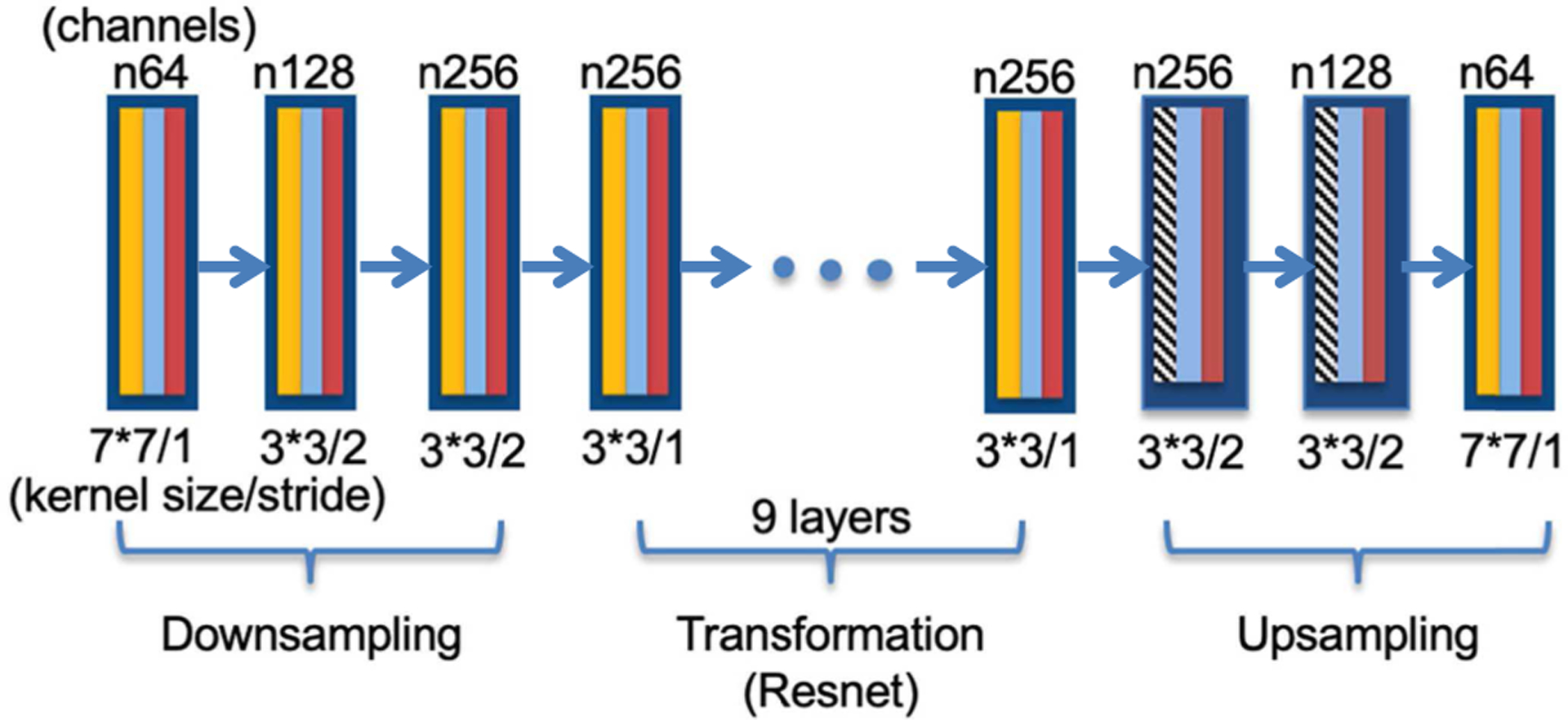
Generator structure of CycleGAN

Fig. 3.

Discriminator structure of CycleGAN

D. GAN-CIRCLE

In a recent work for CT super-resolution and denoising, GAN-CIRCLE [42] was proposed based on the CycleGAN principle. Here is a brief introduction and the details and the default hyperparameters can be found in [42].

1). Loss functions

GAN-CIRCLE uses an additional loss function, Joint Sparsity Transform (JST) loss, as shown below:

$$L_{JST}(G)=\tau \Vert G(x){\Vert }_{TV}+\left(1-\tau \right)\Vert y-G(x){\Vert }_{TV},$$ (8)

where τ is a weighting factor and ∥·∥_TV denotes the total variation (TV) norm. The two terms of this loss function serve two purposes: 1) the first term enforces sparsity on the generated images to remove artifacts; and 2) the second term is to preserve anatomic details by minimizing the difference between y and G (x). Thus, the overall objective function for GAN-CIRCLE becomes:

$$L_{GAN-\mathit{\text{CIRCLE}}}=L_{\mathit{\text{WGAN}}}\left(D_Y,G\right)+L_{\mathit{\text{wGAN}}}\left(D_X,F\right)+\lambda L_{cyc}(G,F)+\mu L_{IDT}(G,F)+v{L}_{JST}(G),$$ (9)

where the GAN losses adopt the Wasserstein distance (for the forward mapping),

$$L_{\mathit{\text{WGAN}}}\left(D_Y,G\right)=E_x\left[D_y(G(x))\right]-E_y\left[D_y(y)\right]+\alpha E_{\widehat{y}}\left[{\left({\Vert {\nabla }_{\widehat{y}}{D}_y(\widehat{y})\Vert }_2-1\right)}^2\right].$$ (10)

The first two terms in the Wasserstein loss function calculate Wasserstein estimation, and the third term penalizes the deviation of the gradient norm of $D_y(\widehat{y})$ from one, $\widehat{y}$ is uniformly sampled along straight lines for pairs of G (x) and y, α is a weighting parameter. A similar Wasserstein GAN loss can be defined for the backward mapping. Note that the JST loss was not used in this work since it did not improve the denoising performance significantly and increases the computation and the number of hyperparameters.

2). Network structures

We summarize the network structures of GAN-CIRCLE based on their shared code at https://github.com/charlesyou999648/GAN-CIRCLE in Fig. 4 and 5. Note that they are slightly different from that described in the paper [42]. GAN-CIRCLE simplifies the generator by shrinking the kernel and channel sizes and adding more bypass connections. It also omits the batch normalization following the convolutional layers in the generator. As shown in Fig. 4, each output feature is garnered at the end of the feature extraction stage, which can preserve information in previous convolutional layers. During upsampling, two-way convolutional layers are first used, then followed by a convolution layer and a deconvolution layer. The discriminator follows the same structure as that in CycleGAN, but with eight convolutional layers as shown in Fig. 5. The block color and style represent the same functions as that in CycleGAN, except for the loss function (using (9) instead of (7)) (green block).

Fig. 4.

Generator structure of GAN-CIRCLE

Fig. 5.

Discriminator structure of GAN-CIRCLE

III. Experimental settings

To evaluate the denoising performance of CycleGAN, IdentityGAN, and GAN-CIRCLE, we performed the whole image-based learning, and then picked the best performer for patch-based training using a real clinical dataset from the 2016 NIH-AAPM-Mayo Clinic Low Dose CT Grand Challenge (https://www.aapm.org/GrandChallenge/LowDoseCT/). Single-image iterative denoising methods, KSVD [26] and BM3D [30], and a paired deep learning denoising method, RED-CNN [33], were also implemented for comparison.

A. Training setup

The low-dose CT dataset contains 10 anonymous patients’ full-dose thoracic and abdominal CT data (close to 6,000 2D images for all patients) and corresponding low-dose (1/4 of the full dose) CT data. An NVIDIA Tesla V100 GPU card is used for computing. The GPU-version PyTorch (version greater than 1.4.0) and Tensorflow (version greater than 1.11) are used to run RED-CNN, CycleGAN, IdentityGAN, and GAN-CIRCLE, respectively.

1). Whole image training

The original images are resized from 512×512 to 256×256 to enable fast whole image-based training. We choose images of the 2^nd to 10^th patient as the training set (5,376 images) and that of the 1^st patient as the test data (560 images). Note that the training images are randomly scrambled, so there is no paired correspondence between the full-dose and low-dose images for each training batch.

2). Patch-based training

Since the original training dataset only has less than 6,000 images, it is necessary to augment the training set to investigate the sample size influence on deep learning models for low-dose CT denoising. Specifically, if 64 × 64 overlapping patches were extracted from the original 512 × 512 images with a stride of 32, each image can produce 255 training patches. The whole process can lead to sufficient data (>1.5 million patches in total) to investigate the influence of the sample size on training performance. Since GAN-CIRCLE with simpler generator structures computes much faster (see Table IV) and has the best denoising performance among the three methods based on cycle-consistent GAN, we use GAN-CIRCLE for experiments in this part. Instead of fixing the training and test data sets, the 10-fold cross-validation is used to get the estimate of expected performance on PSNR and SSIM on 512×512 images.

TABLE IV.

Computation time for different methods (training for each epoch and test for each image)

	RED-CNN	Cycle-GAN	IdentityGAN	GAN-Circle
Train	1.20 min	21.12 min	119.78 min	5.95 min
Test	0.01 sec	0.05 sec	0.04 sec	0.02 sec

First, we investigate the influence of the number of patches on the denoising performance of GAN-CIRCLE. One of 10 patients is used as the test set and the other nine patients are used for training. The number of patches randomly selected from each image is 1, 4, 7, 13, 25, and 50, which leads to a total number of patches approximate 5,000, 21,000, 37,000, 69,000, 134,000, and 268,000 from images of nine training patients (where the exact number depends on the particular test patient selected). It repeats 10 times until each of the 10 patients was used as a test set. The quantitative evaluation metrics are averaged over 10 trials for different numbers of training patches.

Secondly, we investigate the influence of the number of patients on the denoising performance of GAN-CIRCLE. We use one patient as the test data and randomly select 1, 2, 4, and 6 patients in the other patients as the training data. The training is repeated 10 times for each of 10 patients as the test set. The last experiment is the 10-fold cross-validation with one patient as the test data and the other 9 as the training data. Twenty-five patches per image are used to form the training data.

Finally, we conduct two additional experiments to demonstrate the effectiveness of denoising methods using unpaired deep learning: (1) Non-overlapping patient training: the training set comprises FDCT images of patient 2–6 and LDCT images of patient 7–10, and the test data is patient 1; and (2) Non-overlapping organ training: the training set is composed of FDCT images for thoracic slices and LDCT images for abdominal slices of patient 2–9 and the test data is patient 1. In both cases, there is no corresponding FDCT image for the LDCT image.

B. Evaluation Metrics

Two metrics are used to quantitatively evaluate different methods: peak signal-to-noise ratio (PSNR) [49] and structural similarity index (SSIM) [50, 51]. PSNR measures denoising performance by calculating the overall difference between the denoised LDCT image and the original FDCT image and is defined as:

$$\mathit{\text{PSNR}}=10\cdot {\text{log}}_{10}\left(\frac{MA{X}_Y^2}{MSE}\right),$$ (11)

where MSE stands for mean squared error and MAX_Y denotes the maximum intensity value, which was set as 4096 for 12-bit CT images in this work. The MSE is calculated as:

$$MSE=\frac{1}{mn}{\sum }_{i=0}^{m-1}{\sum }_{j=0}^{n-1}{[x(i,j)-y(i,j)]}^2,$$ (12)

where x denotes the LDCT image or the corresponding region of interest (ROI), y is the corresponding FDCT image or ROI, and m and n denote the size of the image or ROI.

In addition to PSNR, the structural similarity index (SSIM) is also used to measure the perceptual similarity between the denoised LDCT and FDCT images:

$$\mathit{\text{SSIM}}(x,y)=\frac{\left(2{\mu }_x{\mu }_y+c_1\right)\left(2{\sigma }_{xy}+c_2\right)}{\left({\mu }_x^2+{\mu }_y^2+c_1\right)\left({\sigma }_x^2+{\sigma }_y^2+c_2\right)},$$ (13)

where, μ_x and μ_y are the averages of x and y, ${\sigma }_x^2$, ${\sigma }_y^2$ and σ_xy are the variance and covariance, and c₁ and c₂ are two variables to stabilize the division operation [50, 51]. The higher PSNR and SSIM represent the better performance. Note that the results calculated on the downsampled 256×256 images in IV.A and B are usually better than those calculated on the original 512×512 images in IV.C and D.

IV. Results

A. Hyperparameter tuning

Base on the metrics defined above, we explore influences of hyperparameters including the learning rate and the regularization factor λ (for the cycle consistency loss), as well as the GAN loss functions (least squares loss vs. Wasserstein loss) by evaluating the test dataset (patient 1). We use fixed 150 epochs. The learning rate is fixed for the first 100 epochs, and then linearly decays to a half for the last 50 epochs. Table I and II show how the combinations of learning rates (LR) and the regularization factor λ (for GAN-CIRCLE with the least squares loss) change the PSNR and SSIM performance, respectively. The large learning rate causes the training divergent, while the small learning rate fails to efficiently update model parameters, thus leading to inferior PSNR and SSIM performance. We chose the learning rate of 1×10⁻⁴ and λ = 100 as the hyperparameters for GAN-CIRCLE for the following experiments unless otherwise stated. For μ, we tested the values of [0, 0.1, 0.5, 0.75, 1]λ and found that the good PSNR could be obtained as long as μ ≠ 0. Thus, we used μ = 0.5λ in the following experiments. For the different loss functions of least squares and Wasserstein, we found that the least squares loss worked better than the Wasserstein loss based on PSNR. Therefore, the least squares loss was used in the following experiments. For CycleGAN and IdentityGAN, a similar search was conducted. The corresponding hyperparameters are LR = 2 × 10⁻⁴ and λ = 10 for CycleGAN, and LR = 2 × 10⁻⁴ and λ = 10 for IdentityGAN. Similarly, we tuned the parameters for KSVD (noise sigma = 0.007), BM3D (noise sigma = 0.009) and RED-CNN (LR = 1 × 10⁻⁵) to get their best PSNR values averaged on all images of patient 1.

TABLE I.

Influence of learning rate and λ on PSNR (dB)

LR/ λ	0.1	1	10	100	500
1×10−5	44.07	44.32	45.15	46.28	46.24
1×10−4	43.30	47.80	47.68	47.90	47.80
1×10−3			Divergent

TABLE II.

Influence of learning rate and λ on SSIM

LR/ λ	0.1	1	10	100	500
1×10−5	0.9637	0.9610	0.9649	0.9686	0.9675
1×10−4	0.9583	0.9696	0.9743	0.9753	0.9747
1×10−3			Divergent

The detailed results (averaged on all image slices of Patient 1) for different methods are listed in Table III. All denoising methods lead to better PSNR and SSIM than the original LDCT images (44.89 dB and 0.9372). GAN-CIRCLE achieves the best performance in PSNR and SSIM, followed closely by RED-CNN. CycleGAN and IdentityGAN also yield decent results. KSVD and BM3D work well on PSNR, but suffer lower SSIM values. Note that the PSNR and SSIM values obtained from our implementation of (unsupervised) GAN-CIRCLE are much higher than that in [42], likely due to the resized images and different parameters used in the calculation of these metrics, such as the dynamic range of converted images and MAX_Y in PSNR. Thus, the head-to-head comparison is not meaningful.

TABLE III.

Quantitative Results Averaged over 560 Test Images of 1^st Patient

Method	PSNR(dB)	SSIM
LDCT	44.89(1.01)	0.9372(0.0165)
KSVD	47.34(0.77)	0.9638(0.0085)
BM3D	47.76 (0.73)	0.9662(0.0075)
RED-CNN	47.82 (0.74)	0.9730(0.0070)
CycleGAN	47.09 (0.98)	0.9717(0.0080)
IdentityGAN	47.59(0.72)	0.9674(0.0085)
GAN-CIRCLE	47.90(0.69)	0.9753(0.0074)

B. Denoised Images

To visualize the denoising performance of different methods, we select one thoracic slice containing the lungs and one abdominal slice containing the liver from the test dataset (patient 1) as shown in Fig. 6 and 8, respectively. The zoomed-in ROIs for details in the lung and the liver are shown in Fig. 7 (red rectangle in Fig. 6a) and 9 (red rectangle in Fig. 8a), respectively. As shown in Fig. 6, the LDCT image shows streak noise compared to the FDCT image. All denoising methods alleviate the streak artifacts. Among them, KSVD and BM3D seem to suppress these artifacts more at the expense of oversmoothing. The deep learning methods not only suppress the noise effectively, but also preserve structural details. The PSNR and SSIM for this slice are listed in the caption. RED-CNN achieves the best quantitative accuracy, closely followed by GAN-CIRCLE. This phenomenon is more apparent in zoomed-in views in Fig. 7. KSVD and BM3D oversmooth the region (e.g. the red circle area) and lead to low PSNR and SSIM. The BM3D image shows smoother looking, but suffers a great loss of details. Thus, its PSNR and SSIM are worse than LDCT, because the parameters of BM3D were tuned for all images of a patient, instead of the current slice. The paired deep learning method, RED-CNN, achieves the best noise removal performance and three un-paired deep learning methods with cycle-consistent GAN perform similarly.

Fig. 6.

A thoracic transverse slice for different methods: (a) Full-dose CT; (b) Low-dose CT (PSNR: 44.64 dB and SSIM: 0.9565); (c) KSVD (46.25 dB and 0.9726); (d) BM3D (46.40 dB and 0.9719); (e) RED-CNN (46.57 dB and 0.9776); (f) CycleGAN (44.72 dB and 0.9756); (g) IdentityGAN (45.71 dB and 0.9619) and (h) GAN-CIRCLE (46.31 dB and 0.9772). (Display window [−1350 150]HU).

Fig. 8.

An abdominal transverse slice for different methods: (a) Full-dose CT; (b) Low-dose CT (PSNR: 43.23 dB and SSIM: 0.9149); (c) KSVD (45.82 dB and 0.9534); (d) BM3D (46.31 dB and 0.9572); (e) RED-CNN (46.23 dB and 0.9606); (f) CycleGAN (45.70 dB and 0.9554); (g) IdentityGAN (45.38 dB and 0.9523) and (h) GAN-CIRCLE (46.21 dB and 0.9611). (Display window [−160 240]HU).

Fig. 7.

The zoomed-in lung region for different methods (the red rectangle in Fig. 6a): (a) Full-dose CT; (b) Low-dose CT (PSNR: 46.78 dB and SSIM: 0.9370); (c) KSVD (47.17 dB and 0.9409); (d) BM3D (46.59 dB and 0.9229); (e) RED-CNN (48.01 dB and 0.9515); (f) CycleGAN (47.55 dB and 0.9479); (g) IdentityGAN (47.17 dB and 0.9437) and (h) GAN-CIRCLE (47.01 dB and 0.9435). (Display window [−1350 150]HU).

The abdominal slice in Fig. 8 shows more organs and structural details. Again, all denoising methods effectively remove the grainy and streak noise and lead to improved PSNR and SSIM. Among all methods, BM3D provides the best PSNR and GAN-CIRCLE yields the best SSIM. BM3D gains an advantage in more uniform regions in this slice although the texture of its denoised image is different from the FDCT image. In the zoomed-in view of Fig. 9 for the liver region, BM3D shows the smoothest look, which strongly boosts its PSNR performance. However, the texture inside the liver is largely lost. The deep learning-based denoising methods have done a decent job on removing the noise while maintaining the texture details. The smoothness of this ROI is in the order of RED-CNN, GAN-CIRCLE, CycleGAN, and IdentityGAN. From these images, we can see that (1) the deep learning-based denoising can adapt to different targets in the images with different noise properties and structural details compared to the conventional methods, which are less adaptive; and (2) the unpaired deep learning methods based on cycle-consistent GAN are comparable to, if not better than, the paired deep learning method on LDCT denoising.

Fig. 9.

The zoomed-in liver region for different methods (the red rectangle in Fig. 8a): a) Full-dose CT; (b) Low-dose CT (PSNR: 41.96 dB and SSIM: 0.6354); (c) KSVD (45.80 dB and 0.7404); (d) BM3D (46.60 dB and 0.7177); (e) RED-CNN (45.92 dB and 0.7363); (f) CycleGAN (45.13 dB and 0.7300); (g) IdentityGAN (44.83 dB and 0.7162) and (h) GAN-CIRCLE (46.07 dB and 0.7423). (Display window [−160 240]HU).

C. The influence of the size of training samples

GAN-CIRCLE has lightweight generators (0.168 million parameters for each generator), which is much more computationally efficient than CycleGAN and IdentityGAN (see Table IV). Furthermore, the hyperparameters were thoroughly investigated and optimized in [36] for patch-based learning. Therefore, we use GAN-CIRCLE to evaluate the influence of the size of training samples using image patches. Note that the PSNR and SSIM results in the following sections are calculated based on 512×512 images, which are different from previous sections using downsampled 256×256 images. The baseline PSNR and SSIM of LDCT images averaged over 10 patients are 40.88 dB(1.22) and 0.8710(0.0387), respectively.

1). The influence of the number of training patches

As the patches extracted from each single 512×512 image increase from 1 to 50, the total training patches increase from about 5,000 to about 268,000. The average PSNR and SSIM values for 10 trails are plotted in Fig. 10 with error bars denoting the standard deviation. These values are significantly greater than the original LDCT values and indicate effective denoising. As can be seen, both PSNR and SSIM values increase with the number of training patches, except for from 4 patches/image to 7 patches/image. It implies that the larger the number of training samples, the better the denoising performance. However, the gain from the increased number of patches per image diminishes as it goes beyond 25 patches/image. The use of 25 patches/image seems to have a good balance between the denoising performance and computational burden.

Fig. 10.

Influence of the number of training patches per image on denoising performance. The horizontal axis denotes the number of patches per image that are randomly extracted from each 512×512 image. Each of 10 patients was used as the test data once and the results were averaged over 10 trials for each data point.

2). The influence of the number of patients for training

In this part, the number of patches per image is fixed as 25. As the number of patients for training increases from one to nine, both average PSNR and SSIM values increase as shown in Fig. 11. Note that the data of every patient is served as the test data once for each condition of the number of training patients (1, 2, 4, 6, and 9). The error bar denotes the standard deviation of 10 trials. The largest increase is from one patient to two patients. Afterward, the increase becomes marginal. It demonstrates that the sufficient patient variety can significantly improve deep learning based LDCT denoising. However, this improvement measured by PSNR and SSIM may reach a plateau at a certain number of training patients, e.g. four patients for the current dataset.

Fig. 11.

Influence of the number of patients in training (the horizontal axis) on denoising performance. Twenty-five patches are randomly extracted from each 512 × 512 image. Each of 10 patients was used as the test data once and the results were averaged over 10 trials for each data point.

D. Totally non-overlapping training

For non-overlapping patient training, the PSNR and SSIM are 43.31 dB and 0.9259, respectively. For non-overlapping organ training, the PNSR and SSIM are 43.47 dB and 0.9262, respectively. Even though there are no counterparts of FDCT images and LDCT images in training, GAN-CIRCLE is able to extract useful features to effectively remove noise. These two values are better than the original LDCT values (PSNR: 40.08 dB; SSIM: 0.8541), mixed training with one patient (PSNR: 43.25 dB; SSIM: 0.9236), and comparable to mixed training with four-patients (PSNR: 43.50 dB; SSIM: 0.9268). The mixed training means that the FDCT and LDCT images of the same patient are used in the training although the one-to-one correspondence is scrambled and not utilized. One abdominal slice is shown in Fig. 12. Even without counterparts of FDCT and LDCT images, non-overlapping training of GAN-CIRCLE effectively suppresses noise and achieves similar performance to the mixed training with four patients. This result provides preliminary evidence that large patient data without one-to-one correspondence, i.e. no need of registration or alignment, could be utilized for effective LDCT denoising through the cycle consistent adversarial learning.

Fig. 12.

An abdominal transverse slice for (a) Full-dose CT; (b) Low-dose CT (PSNR: 38.28 dB and SSIM: 0.7960); (c) 1-patient mixed training (41.47 dB and 0.8891); (d) 4-patient mixed training (41.81 dB and 0.8952); (e) Non-overlapping patient training (41.75 dB and 0.8924); and (f) Non-overlapping organ training (41.74 dB and 0.8928). (Display window [−160 240]HU).

E. Network complexity and computation time

Three variants, CycleGAN [41], GAN-CIRCLE [42], and IdentityGAN [43], have been proposed for LDCT denoising or super-resolution. Their network structures are at different complexity levels: 11.378 million parameters for one generator in CycleGAN, 0.168 million in GAN-CIRCLE, and 6.477 million for IdentityGAN. The training of deep learning-based methods for LDCT denoising is time consuming. The training time (min per epoch) and the test time (sec per slice) for the whole 256×256 image training are listed in Table IV using NVIDIA Tesla V100. For patch-based training, GAN-CIRCLE (134,400 64 × 64 patches by extracting 25 patches per image and a total of nine patients) takes about 23.5 hours for 150 epochs with a batch size of 40 on the NVIDIA Tesla V100. The computation time linearly increases with the number of training patches. Once the training is done, the deep learning-based methods are much faster than KSVD and BM3D to denoise images (see Test time in Table IV).

V. Discussion and Conclusions

In this work, we developed a novel image-to-image translation method based on CycleGAN and compared it with two other variants for low-dose CT image denoising. These cycle-consistent based GAN methods do not require aligned image pairs and yet provide the denoising performance comparable to the paired training, RED-CNN, which makes them particularly valuable to utilize abundant unpaired training samples. Among three variants, CycleGAN, IdentityGAN, and GAN-CIRCLE, the latter uses a lightweight network and achieves the best denoising performance for the NIH-AAPM-Mayo Clinic Low Dose CT data. The much more complicated network structures in CycleGAN and IdentityGAN do not improve the denoising performance, but demand much more computational resources. Although the LDCT data used in this study were synthesized using a validated noise insertion method [52], further investigation using real LDCT data would be preferred to verify the findings in this work and to improve unpaired deep learning methods. However, these studies are out of the scope of this work and will be investigated in the future.

Using patch-based training where a large number of training samples become available, we investigated the influence of the size of training samples and the variety of training patients on denoising performance of the unpaired deep learning method. Our results show that increasing the number of training patches and the number of patients can improve the denoising performance as shown in Fig. 10 and 11. The increase of the number of training patches saturates the improvement for 25 random patches per image even though more patches per image are available. This is likely due to the information carried by the training data (of nine patients) is sufficiently represented by these patches. With further increase of the patches, the redundant information has none or little help on better training. The extra information introduced by new patient data can also boost the performance of deep learning based denoising as shown in Fig. 11. However, the benefit of additional patient data diminishes after using more than four patients. It seems that the current network structures can use less than nine patient data to achieve a denoising performance close to the optimum. We attempted to add the layers of GAN-CIRCLE and obtained a similar PSNR performance. Whether the network structures can be further optimized to achieve better denoising performance or the upper bound of denoising for the current dataset has been reached is worth further investigation.

The semi-unsupervised deep learning methods (using unpaired images), such as cycle-consistent GAN, have a unique advantage over the supervised deep learning methods (using paired images) to include more training data since no alignment of images in two domains is needed. (Note that we call this unpaired learning as “semi-unsupervised” learning because it still needs labels to denote which domain the training data belong to, while the unpaired learning was simply called “unsupervised” learning in [42] where “semi-unsupervised” was used for mixed paired and unpaired learning.) Although the LDCT and FDCT data in training were scrambled to void direct use of image pairs, the LDCT and FDCT pairs did exist in the training data, which could provide information leading to spurious good performance. The additional non-overlapping experiment was conducted to demonstrate the effectiveness of cycle-consistent GAN for unpaired training without counterparts in two domains, i.e. LDCT and FDCT, in terms of both patient-wise non-overlapping and organ-wise non-overlapping (Fig. 12). These promising results show that unpaired learning based on cycle-consistent GAN can provide a powerful tool to use a large number of images in two domains without the requirement of alignment.

In future work, we will investigate how to systematically optimize network architectures and hyperparameters since the empirical trial-and-error is not only sub-optimal, but also is unbearably time consuming. The investigation of the upper bound of denoising performance for the supervised deep learning methods (using paired images) and the semi-unsupervised deep learning methods (using unpaired images) based on cycle-consistent GAN for low-dose CT denoising will be another interesting direction. With a sufficiently large number of patient data, we envision that the unpaired learning can approach and go beyond the performance of the supervised learning.

References

- [1].Brenner DJ and Hall EJ, “Computed tomography–an increasing source of radiation exposure,” The New England journal of medicine, vol. 357, no. 22, pp. 2277–84, November 29 2007, doi: 10.1056/NEJMra072149. [DOI] [PubMed] [Google Scholar]
- [2].de Gonzalez AB and Darby S, “Risk of cancer from diagnostic X-rays: estimates for the UK and 14 other countries,” The lancet, vol. 363, no. 9406, pp. 345–351, 2004. [DOI] [PubMed] [Google Scholar]
- [3].La Rivière PJ, Bian J, and Vargas PA, “Penalized-likelihood sinogram restoration for computed tomography,” IEEE transactions on medical imaging, vol. 25, no. 8, pp. 1022–1036, 2006. [DOI] [PubMed] [Google Scholar]
- [4].Wang G, Snyder DL, O’Sullivan JA, and Vannier MW, “Iterative deblurring for CT metal artifact reduction,” IEEE transactions on medical imaging, vol. 15, no. 5, pp. 657–664, 1996. [DOI] [PubMed] [Google Scholar]
- [5].La Riviere PJ, “Penalized-likelihood sinogram smoothing for low-dose CT,” Med Phys, vol. 32, no. 6, pp. 1676–83, June 2005, doi: 10.1118/1.1915015. [DOI] [PubMed] [Google Scholar]
- [6].Chen Y et al. , “Thoracic low-dose CT image processing using an artifact suppressed large-scale nonlocal means,” Physics in Medicine & Biology, vol. 57, no. 9, pp. 2667–88, 2012. [DOI] [PubMed] [Google Scholar]
- [7].Giraldo JCR, Kelm ZS, Guimaraes LS, and Yu L, “Comparative study of two image space noise reduction methods for computed tomography: Bilateral filter and nonlocal means,” vol. 2009, pp. 3529–3532, 2009. [DOI] [PubMed] [Google Scholar]
- [8].Li Z et al. , “Adaptive nonlocal means filtering based on local noise level for CT denoising,” Medical Physics, vol. 41, no. 1, pp. 011908–011908, 2014. [DOI] [PubMed] [Google Scholar]
- [9].Ma J et al. , “Low-dose computed tomography image restoration using previous normal-dose scan,” Medical Physics, vol. 38, no. 10, pp. 5713–31, 2011. [DOI] [PMC free article] [PubMed] [Google Scholar]
- [10].Xu W, Ha S, and Mueller K, “Database-assisted low-dose CT image restoration,” Medical Physics, vol. 40, no. 3, 2013. [DOI] [PubMed] [Google Scholar]
- [11].Geraldo RJ, Cura LM, Cruvinel PE, and Mascarenhas ND, “Low dose CT filtering in the image domain using MAP algorithms,” IEEE Transactions on Radiation and Plasma Medical Sciences, vol. 1, no. 1, pp. 56–67, 2017. [Google Scholar]
- [12].Hasan AM, Melli A, Wahid KA, and Babyn P, “Denoising low-dose CT images using multiframe blind source separation and block matching filter,” IEEE Transactions on Radiation and Plasma Medical Sciences, vol. 2, no. 4, pp. 279–287, 2018. [Google Scholar]
- [13].Chen GH, Tang J, and Leng S, “Prior image constrained compressed sensing (PICCS): a method to accurately reconstruct dynamic CT images from highly undersampled projection data sets,” Med Phys, vol. 35, no. 2, pp. 660–3, February 2008, doi: 10.1118/1.2836423. [DOI] [PMC free article] [PubMed] [Google Scholar]
- [14].Ouyang L, Solberg T, and Wang J, “Noise Reduction in Low-Dose Cone Beam CT by Incorporating Prior Volumetric Image Information,” Medical Physics, vol. 39, no. 5, pp. 2569–77, 2012. [DOI] [PubMed] [Google Scholar]
- [15].Sidky EY and Pan X, “Image reconstruction in circular cone-beam computed tomography by constrained, total-variation minimization,” Phys Med Biol, vol. 53, no. 17, pp. 4777–807, September 7 2008, doi: 10.1088/0031-9155/53/17/021. [DOI] [PMC free article] [PubMed] [Google Scholar]
- [16].Stayman JW, Dang H, Ding Y, and Siewerdsen JH, “PIRPLE: a penalized-likelihood framework for incorporation of prior images in CT reconstruction,” Physics in Medicine & Biology, vol. 58, no. 21, pp. 7563–82, 2013. [DOI] [PMC free article] [PubMed] [Google Scholar]
- [17].Thibault JB, Sauer KD, Bouman CA, and Hsieh J, “A three-dimensional statistical approach to improved image quality for multislice helical CT,” Med Phys, vol. 34, no. 11, pp. 4526–44, November 2007, doi: 10.1118/1.2789499. [DOI] [PubMed] [Google Scholar]
- [18].Wang J, Li T, Lu H, and Liang Z, “Penalized weighted least-squares approach to sinogram noise reduction and image reconstruction for low-dose X-ray computed tomography,” IEEE transactions on medical imaging, vol. 25, no. 10, pp. 1272–83, October 2006, doi: 10.1109/42.896783. [DOI] [PMC free article] [PubMed] [Google Scholar]
- [19].Yu H, Zhao S, Hoffman EA, and Wang G, “Ultra-low dose lung CT perfusion regularized by a previous scan,” Academic radiology, vol. 16, no. 3, pp. 363–73, March 2009, doi: 10.1016/j.acra.2008.09.003. [DOI] [PMC free article] [PubMed] [Google Scholar]
- [20].Zhang H, Huang J, Ma J, and Bian Z, “Iterative Reconstruction for X-Ray Computed Tomography Using Prior-Image Induced Nonlocal Regularization,” Biomedical Engineering IEEE Transactions on, vol. 61, no. 9, pp. 2367–78, 2014. [DOI] [PMC free article] [PubMed] [Google Scholar]
- [21].Tian Z, Jia X, Yuan K, Pan T, and Jiang SB, “Low-dose CT reconstruction via edge-preserving total variation regularization,” Physics in Medicine & Biology, vol. 56, no. 18, p. 5949, 2011. [DOI] [PMC free article] [PubMed] [Google Scholar]
- [22].Zhang Y, Wang Y, Zhang W, Lin F, Pu Y, and Zhou J, “Statistical iterative reconstruction using adaptive fractional order regularization,” Biomedical optics express, vol. 7, no. 3, pp. 1015–1029, 2016. [DOI] [PMC free article] [PubMed] [Google Scholar]
- [23].Zhang Y, Zhang W, Lei Y, and Zhou J, “Few-view image reconstruction with fractional-order total variation,” JOSA A, vol. 31, no. 5, pp. 981–995, 2014. [DOI] [PubMed] [Google Scholar]
- [24].Zhang Y, Zhang WH, Chen H, Yang ML, Li TY, and Zhou JL, “Few-view image reconstruction combining total variation and a high-order norm,” International Journal of Imaging Systems and Technology, vol. 23, no. 3, pp. 249–255, 2013. [Google Scholar]
- [25].Zeng GL and Wang W, “Does Noise Weighting Matter in CT Iterative Reconstruction?,” IEEE transactions on radiation and plasma medical sciences, vol. 1, no. 1, pp. 68–75, 2017. [DOI] [PMC free article] [PubMed] [Google Scholar]
- [26].Aharon M, Elad M, and Bruckstein A, “K-SVD: An Algorithm for Designing Overcomplete Dictionaries for Sparse Representation,” IEEE Transactions on Signal Processing, vol. 54, no. 11, pp. 4311–4322, 2006. [Google Scholar]
- [27].Chen Y et al. , “Bayesian statistical reconstruction for low-dose X-ray computed tomography using an adaptive-weighting nonlocal prior,” Computerized Medical Imaging and Graphics, vol. 33, no. 7, pp. 495–500, 2009. [DOI] [PubMed] [Google Scholar]
- [28].Ma J et al. , “Iterative image reconstruction for cerebral perfusion CT using a pre-contrast scan induced edge-preserving prior,” Physics in Medicine & Biology, vol. 57, no. 22, pp. 7519–7542, 2012. [DOI] [PMC free article] [PubMed] [Google Scholar]
- [29].Zhang Y, Xi Y, Yang Q, Cong W, Zhou J, and Wang G, “Spectral CT reconstruction with image sparsity and spectral mean,” IEEE transactions on computational imaging, vol. 2, no. 4, pp. 510–523, 2016. [DOI] [PMC free article] [PubMed] [Google Scholar]
- [30].Dabov K, Foi A, Katkovnik V, and Egiazarian K, “Image denoising by sparse 3-D transform-domain collaborative filtering,” IEEE Transactions on image processing, vol. 16, no. 8, pp. 2080–2095, 2007. [DOI] [PubMed] [Google Scholar]
- [31].Chen H et al. , “Low-dose CT denoising with convolutional neural network,” in 2017 IEEE 14th International Symposium on Biomedical Imaging (ISBI 2017), 2017: IEEE, pp. 143–146. [Google Scholar]
- [32].Chen H et al. , “Low-dose CT via convolutional neural network,” Biomedical optics express, vol. 8, no. 2, pp. 679–694, 2017. [DOI] [PMC free article] [PubMed] [Google Scholar]
- [33].Chen H et al. , “Low-Dose CT with a Residual Encoder-Decoder Convolutional Neural Network (RED-CNN),” IEEE transactions on medical imaging, vol. 36, no. 12, pp. 2524–2535, 2017. [Online]. Available: https://128.84.21.199/pdf/1702.00288v1.pdf. [DOI] [PMC free article] [PubMed] [Google Scholar]
- [34].Kang E, Min J, and Ye JC, “A deep convolutional neural network using directional wavelets for low-dose X-ray CT reconstruction,” Medical Physics, vol. 44, no. 10, 2017. [DOI] [PubMed] [Google Scholar]
- [35].Kadimesetty VS, Gutta S, Ganapathy S, and Yalavarthy PK, “Convolutional neural network-based robust denoising of low-dose computed tomography perfusion maps,” IEEE Transactions on Radiation and Plasma Medical Sciences, vol. 3, no. 2, pp. 137–152, 2018. [Google Scholar]
- [36].Goodfellow I et al. , “Generative adversarial nets,” in Advances in neural information processing systems, 2014, pp. 2672–2680. [Google Scholar]
- [37].Mirza M and Osindero S, “Conditional generative adversarial nets,” arXiv preprint arXiv:1411.1784, 2014. [Google Scholar]
- [38].Wolterink JM, Leiner T, Viergever MA, and Išgum I, “Generative adversarial networks for noise reduction in low-dose CT,” IEEE transactions on medical imaging, vol. 36, no. 12, pp. 2536–2545, 2017. [DOI] [PubMed] [Google Scholar]
- [39].Yang Q et al. , “Low-dose CT image denoising using a generative adversarial network with Wasserstein distance and perceptual loss,” IEEE transactions on medical imaging, vol. 37, no. 6, pp. 1348–1357, 2018. [DOI] [PMC free article] [PubMed] [Google Scholar]
- [40].Isola P, Zhu J-Y, Zhou T, and Efros AA, “Image-to-image translation with conditional adversarial networks,” in Proceedings of the IEEE conference on computer vision and pattern recognition, 2017, pp. 1125–1134. [Google Scholar]
- [41].Zhu J-Y, Park T, Isola P, and Efros AA, “Unpaired image-to-image translation using cycle-consistent adversarial networks,” in Proceedings of the IEEE international conference on computer vision, 2017, pp. 2223–2232. [Google Scholar]
- [42].You C et al. , “CT super-resolution GAN constrained by the identical, residual, and cycle learning ensemble (GAN-CIRCLE),” IEEE transactions on medical imaging, vol. 39, no. 1, pp. 188–203, 2019. [DOI] [PMC free article] [PubMed] [Google Scholar]
- [43].Kang E, Koo HJ, Yang DH, Seo JB, and Ye JC, “Cycle-consistent adversarial denoising network for multiphase coronary CT angiography,” Medical physics, vol. 46, no. 2, pp. 550–562, 2019. [DOI] [PubMed] [Google Scholar]
- [44].Wang J et al. , “An experimental study on the noise properties of x-ray CT sinogram data in Radon space,” Physics in Medicine & Biology, vol. 53, no. 12, p. 3327, 2008. [DOI] [PMC free article] [PubMed] [Google Scholar]
- [45].Kingma D and Ba J, “Adam: A method for stochastic optimization,” in Int. Conf. Learning Representations, 2015. [Google Scholar]
- [46].Krizhevsky A, Sutskever I, and Hinton GE, “Imagenet classification with deep convolutional neural networks,” in Advances in neural information processing systems, 2012, pp. 1097–1105. [Google Scholar]
- [47].Mao X, Li Q, Xie H, Lau RY, Wang Z, and Paul Smolley S, “Least squares generative adversarial networks,” in Proceedings of the IEEE International Conference on Computer Vision, 2017, pp. 2794–2802. [Google Scholar]
- [48].He K, Zhang X, Ren S, and Sun J, “Deep residual learning for image recognition,” in Proceedings of the IEEE conference on computer vision and pattern recognition, 2016, pp. 770–778. [Google Scholar]
- [49].Huynh-Thu Q and Ghanbari M, “Scope of validity of PSNR in image/video quality assessment,” Electronics letters, vol. 44, no. 13, pp. 800–801, 2008. [Google Scholar]
- [50].Hore A and Ziou D, “Image quality metrics: PSNR vs. SSIM,” in 2010 20th International Conference on Pattern Recognition, 2010: IEEE, pp. 2366–2369. [Google Scholar]
- [51].Wang Z, Bovik AC, Sheikh HR, and Simoncelli EP, “Image quality assessment: from error visibility to structural similarity,” IEEE transactions on image processing, vol. 13, no. 4, pp. 600–612, 2004. [DOI] [PubMed] [Google Scholar]
- [52].Yu L, Shiung M, Jondal D, and McCollough CH, “Development and validation of a practical lower-dose-simulation tool for optimizing computed tomography scan protocols,” Journal of computer assisted tomography, vol. 36, no. 4, pp. 477–487, 2012. [DOI] [PubMed] [Google Scholar]