Sensitivity assessment and optimal economic evaluation of a new COVID-19 compartmental epidemic model with control interventions

Abstract

Optimal economic evaluation is pivotal in prioritising the implementation of non-pharmaceutical and pharmaceutical interventions in the control of diseases. Governments, decision-makers and policy-makers broadly need information about the effectiveness of a control intervention concerning its cost-benefit to evaluate whether a control intervention offers the best value for money. The outbreak of COVID-19 in December 2019, and the eventual spread to other parts of the world, have pushed governments and health authorities to take drastic socioeconomic, sociocultural and sociopolitical measures to curb the spread of the virus, SARS-CoV-2. To help policy-makers, health authorities and governments, we propose a Susceptible, Exposed, Asymptomatic, Quarantined asymptomatic, Severely infected, Hospitalized, Recovered, Recovered asymptomatic, Deceased, and Protective susceptible (individuals who observe health protocols) compartmental structure to describe the dynamics of COVID-19. We fit the model to real data from Ghana and Egypt to estimate model parameters using standard incidence rate. Projections for disease control and sensitivity analysis are presented using MATLAB. We noticed that multiple peaks (waves) of COVID-19 for Ghana and Egypt can be prevented if stringent health protocols are implemented for a long time and/or the reluctant behaviour on the use of protective equipment by individuals are minimized. The sensitivity analysis suggests that: the rate of diagnoses and testing, the rate of quarantine through doubling enhanced contact tracing, adhering to physical distancing, adhering to wearing of nose masks, sanitizing-washing hands, media education remains the most effective measures in reducing the control reproduction number ${\mathcal{R}}_c,$ to less than unity in the absence of vaccines and therapeutic drugs in Ghana and Egypt. Optimal control and cost-effectiveness analysis are rigorously studied. The main finding is that having two controls (transmission reduction and case isolation) is better than having one control, but is economically expensive. In case only one control is affordable, then transmission reduction is better than case isolation. Hopefully, the results of this research should help policy-makers when dealing with multiple waves of COVID-19.

1. Introduction

Coronaviruses are one of a group of RNA viruses that infect animals and humans, primarily the upper respiratory and gastrointestinal tract, which has recently caused a major illness in humans [1]. In 2002 there emerged the Severe Acute Respiratory Syndrome (SARS) in Southern China, causing about 8,098 infections, and 774 deaths in almost 17 countries [2]. Also, there emerged Middle East Respiratory Syndrome (MERS) in 2012, with 536 Laboratory confirmed cases and 145 deaths [3]. In late December 2019, a new coronavirus emerged, causing pneumonia in people, and have been named COVID-19 (caused by novel SARS-CoV-2 coronavirus) [1]. The outbreak of the COVID-19 has raised a lot of health and economic concerns for health authorities and governments in the world.

The preventive measures that were used for other coronaviruses (SARS and MERS) are being used to reduce the spreading rate of the COVID-19. Other novel measures are also being used, such as travel restrictions, stay at home, and lockdowns [1], [4]. The World Health Organization (WHO) has recommended the following preventive measures to reduce the general risk of acute respiratory infections while travelling, or migrating from affected areas: (i) Avoiding close contact with people suffering from acute respiratory infections, (ii) frequent hand washing, (iii) avoiding farm and wild animals, (iv) wearing of face-mask, (v) avoiding crowded places, (vi) staying at home except in order to attend to necessities and (vii) self-isolation, even with minor symptoms, and so on [1], [5], [6].

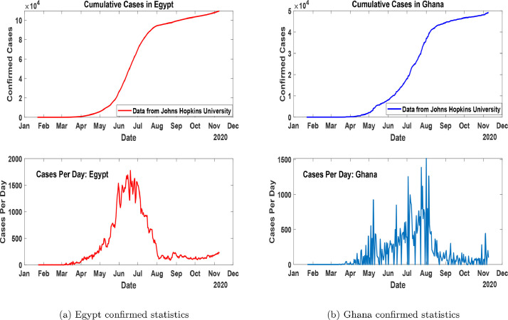
In Africa, the first case was reported on February 14, 2020, in Egypt [7], [8]. The first case of COVID-19 in Ghana was recorded on March 12, 2020 [9]. Fig. 1 (a) and 1(b) shows the cumulative and daily trajectories of COVID-19 for Egypt and Ghana after the first recorded cases to November 10, 2020.

Fig. 1.

Confirmed statistics of cumulative and daily cases in Egypt and Ghana as at November 10, 2020.

In the light of studying the dynamics of COVID-19, El-Ghitany [10] studied, a short-term forecast scenario for the COVID-19 epidemic and allocated hospital readiness in Egypt and concluded that cases are expected to continue on the rise and expected to start to decline late in May 2020. Frost et al. [11] proposed a $SECIR$ model to study the disease in Africa and showed the relative importance of lockdown measures (social distancing interventions). Zhao et al. [12], studied an adjusted $SEIR$ model to predict the COVID-19 spread in South Africa, Egypt, Algeria, Nigeria, Senegal, and Kenya. Asamoah et al. [13], proposed a compartmental model to study the effects of immigration on the spread of COVID-19. Sun et al.[14] studied a $SEIQR$ model to predict the transmission dynamics of COVID-19 in Wuhan, China with the effects of lockdown and medical resources. They found out that, lockdowns result in fewer infected people in Wuhan, leading to a lower infection rate in other cities in China. During the spikes of new cases after the first recorded cases in Ghana and Egypt, the aforementioned countries implemented similar control measures to curb the spread of the COVID-19, such measures included: (i) Protecting susceptible individuals, thus through lockdown directives and safety health protocols of the use of nose masks, proper hand-washing and physical distancing, the use of other PPEs, personal hygiene, physical distancing, etc, (ii) Quarantine of asymptomatic individuals due to contact tracing, (iii) Testing and diagnosing of symptomatic individuals, (iv) Hospitalization (isolations) policy. But, to the best of our knowledge, these control measures received limited mathematical and economic evaluation attention in the previous mathematical studies. Hence, we propose a new mathematical model involving a system of ordinary differential equations to study the transmission dynamics of the COVID-19 pandemic using real data within the time window March 12, 2020, to October 31, 2020, for Ghana; and February 12, 2020, to October 31, 2020, for Egypt, to complement the already existing models on estimating the control reproduction numbers for the pandemic within the stated time window in some African regions. We also aim to assess the impact of the control measures used in these countries using sensitivity and optimal control analysis. We hope that this study provides some insight on how to minimize cost and also increase non-pharmaceutical control measures to prevent the COVID-19 in the case of a second wave or multiple waves.

The rest of the paper is organized as follows: In Section 2 the model under consideration is formulated, and control reproduction number ${\mathcal{R}}_c,$ is obtained. In Section 3, the parameter estimation and some numerical simulations of confirmed cases in Ghana and Egypt are presented. Section 4 contains the sensitivity analysis for the aforementioned countries. The domain of Section 5 contains the optimal control formulation, approaches, economic and effectiveness evolution, and lastly, in Section 7, we give concluding remarks.

2. Model formulation

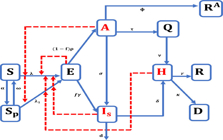
In this model, we extend the generalized $SEIR$ epidemic model to a $SEAQ{I}_{s}HR{R}^{A}D{S}_p$ model. We assumed that births and natural death have no impact on the dynamics due to the relatively fast spread of COVID-19 and the short period considered in this study. The model focuses on two distinct groups of Susceptible individuals: $S,$ the most susceptible individuals who do not adhere to lockdown directives and safety health protocols of the use of nose masks, proper hand-washing and physical distancing at time $t,$ and $S_p,$ the less susceptible individuals who partially or obey the government policy of lockdown, adhere to the safety health protocols (facemasks, PPE, hygiene, physical distancing, etc, i.e. all non-pharmaceutical interventions) at time $t$. The rest of the population is compartmentalized as follows: $E$ are the exposed individuals at time $t,$ $A$ are the asymptomatic (and/or mildly symptomatic) individuals at time $t,$ $I_s$ are the severely symptomatic and infectious individuals at time $t,$ $Q$ are the quarantined asymptomatic individuals (i.e. travellers from epidemic countries and traced resident contacts of infected persons), $H$ are the reported hospitalized and/or isolated individuals, $R$ are the reported recovered individuals, $D$ records the individuals who have unfortunately lost their lives due to COVID-19, $R^A$ are the asymptomatic individuals who recover but are not reported. Fig. 2 shows the epidemiological dynamics of the proposed model.

Fig. 2.

Prototypical patterns of the model formulation.

The transmission rate due to effective contact of $S$ with $E,A,I_s,H$ is denoted as $\lambda =\beta \frac{({\eta }_{0}E+{\eta }_{1}A+I_s+{\eta }_{2}H)S}{N-Q-D}$. Also, let ${\lambda }_1=(1-{\beta }_1)\beta \frac{({\eta }_{0}E+{\eta }_{1}A+I_s+{\eta }_{2}H)S_P}{N-Q-D}$ be the reduced transmission rate of infection of $S_p$ due to effective contact with $E,A,I_s,H,$ where parameters ${\eta }_i,i=0,1,2,0\le {\eta }_i<1$ are the relative COVID-19 transmissibility of $E,$ $A,$ and $H$ respectively. The parameter, $\beta$ is the transmission rate from the infectious classes to the Susceptible class (S and $S_p$). Due to fact that new cases continue to be reported even after the lockdowns and use of other safety health protocols, we assume that the $S_p$ class can get infected, albeit at a reduced rate of $(1-{\beta }_1)$ with $0\le {\beta }_1<1$.

The parameters $r$ and $\kappa$ are COVID-19 recovery rate and disease-induced mortality rate for the $H$ class respectively. The other parameters used in Fig. 2 are as fellows, $\alpha$ is the rate of protection of susceptible individuals, thus, $0\le \alpha <1,$ $\omega$ is the rate at which protected susceptible individuals rejoin the main susceptible class, $\rho$ is the rate of exposure to the asymptomatic class, $\gamma$ is the rate of progression from severely infected to hospitalization, $f$ is the proportion of individuals who develop severe symptoms, $\tau$ is the rate of quarantine, varied and optimized to fit the existing data [15], $\sigma$ is the rate of progression of asymptomatic to severely infected class, also varied to fit the existing data [15], $\delta$ and $\nu$ represent the rate of hospitalization or confinement to isolation centre of the quarantined class and severely infected class respectively, with the notion that $\delta \ge \nu .$ The rate of natural recovery of mildly symptomatic individuals is denoted by $\varphi ,$ the death rate of COVID-19 in the $I_s$ class is denoted by $d$. Based on the above assumptions, the set of differential equations in (1) describe the dynamics of the proposed model.

$$\begin{array}{c}\hfill \{\begin{array}{c}\frac{\mathit{dS}}{\mathit{dt}}=-\beta \frac{({\eta }_{0}E+{\eta }_{1}A+I_s+{\eta }_{2}H)S}{N-Q-D}-\alpha S+\omega S_p,\hfill \\ \frac{\mathit{dE}}{\mathit{dt}}=\beta \frac{({\eta }_{0}E+{\eta }_{1}A+I_s+{\eta }_{2}H)S}{N-Q-D}+(1-{\beta }_1)\beta \frac{({\eta }_{0}E+{\eta }_{1}A+I_s+{\eta }_{2}H)S_p}{N-Q-D}\hfill \\ -(1-f)\rho E-f\gamma E,\hfill \\ \frac{\mathit{dA}}{\mathit{dt}}=(1-f)\rho E-\tau A-\sigma A-\varphi A,\hfill \\ \frac{\mathit{dQ}}{\mathit{dt}}=\tau A-\nu Q,\hfill \\ \frac{d{I}_s}{\mathit{dt}}=f\gamma E+\sigma A-(\delta +d)I_s,\hfill \\ \frac{\mathit{dH}}{\mathit{dt}}=\nu Q+\delta I_s-\mathit{rH}-\kappa H,\hfill \\ \frac{d{R}^A}{\mathit{dt}}=\varphi A,\hfill \\ \frac{\mathit{dR}}{\mathit{dt}}=\mathit{rH},\hfill \\ \frac{\mathit{dD}}{\mathit{dt}}=\kappa H,\hfill \\ \frac{d{S}_p}{\mathit{dt}}=\alpha S-\omega S_p-(1-{\beta }_1)\beta \frac{({\eta }_{0}E+{\eta }_{1}A+I_s+{\eta }_{2}H)S_p}{N-Q-D}.\hfill \end{array}\end{array}$$ (1)

With initial conditions

$$S\left(0\right)=S_0\ge 0,E\left(0\right)=E_0\ge 0,A\left(0\right)=A_0\ge 0,\rho \ge \gamma ,$$

$$Q\left(0\right)=Q_0\ge 0,I_s\left(0\right)={I_s}_0\ge 0,H\left(0\right)=H_0\ge 0,$$

$$R\left(0\right)=R_0\ge 0,R^A\left(0\right)=R_0^A\ge 0,D\left(0\right)=D_0\ge 0,S_p\left(0\right)=S_{p_0}\ge 0.$$

2.1. Basic properties

To carry out the simulations of the model (1) and then assess the economic evaluations of the various control interventions, it is important to study the fundamental properties of the proposed model [16]. Thus, the feasible region of the model is given as

$${\Omega }_N=\left\{(S,E,A,Q,I_s,H,R,D,S_p\le N\left(0\right))\right\}.$$

Which is positively-invariant; that is the solutions of model (1) that start in ${\Omega }_N$ stays in ${\Omega }_N$ as time progresses $(t>0)$ and also “attract all solutions of the model” [16], [17]. Therefore, the proposed model is well-posed mathematically and epidemiologically in the feasible region ${\Omega }_N$ [16], [17], [18].

There is a disease-free equilibrium (DFE) with $(S,E,A,Q,I_s,H,R,R^A,D,S_p)$. To obtain the disease-free equilibrium, we set the right-hand side of model (1) to zero. Hence, the disease-free equilibrium of model (1) is given by:

$${\mathcal{E}}^0=(S^{*},E^{*},A^{*},Q^{*},I_s^{*},H^{*},R^{*},{R^A}^{*},D^{*},S_p^{*})=(N\left(0\right)-S_p^{*},0,0,0,0,0,0,0,0,S_p^{*}),$$

where, $N\left(0\right)$ represent the total initial population, $0<S^{*}\le N\left(0\right),$ $0\le S_p^{*}<N\left(0\right),$ and $0<S^{*}+S_p^{*}\le N\left(0\right)$ [16]. To calculate the control reproduction number and the asymptotic stability of the disease-free equilibrium, we used the van den Driessche and Watmough [19] next-generation method, thus considering the compartments $(E,A,I_s,H),$ with the assumptions that the total population is entirely susceptible. Then, the control reproduction number is obtained as

$$\begin{array}{cc}\hfill {\mathcal{R}}_c=& \underset{\text{secondary}\text{infection}\text{seeded}\text{by}\mathit{E}\text{state}}{\underbrace{\frac{((1-{\beta }_1)\beta +\beta ){\eta }_0}{(f\gamma +(1-f\left)\rho \right)}}}+\underset{\text{secondary}\text{infection}\text{seeded}\text{by}\mathit{A}\text{state}}{\underbrace{\frac{((1-{\beta }_1)\beta +\beta ){\eta }_1(1-f)\rho }{(f\gamma +(1-f\left)\rho \right)(\sigma +\tau +\varphi )}}}\hfill \\ & +\underset{\text{secondary}\text{infection}\text{seeded}\text{by}\mathit{I}\text{state}}{\underbrace{\frac{((1-{\beta }_1)\beta +\beta )[(1-f)\rho \sigma +f\gamma (\sigma +\tau +\varphi )]}{(d+\delta )(f\gamma +(1-f\left)\rho \right)(\sigma +\tau +\varphi )}}}\hfill \\ & +\underset{\text{secondary}\text{infection}\text{seeded}\text{by}\mathit{H}\text{state}}{\underbrace{\frac{((1-{\beta }_1)\beta +\beta ){\eta }_2\delta [f\gamma (\sigma +\tau +\varphi )+(1-f)\rho \sigma ]}{(d+\delta )(f\gamma +(1-f\left)\rho \right)(\sigma +\tau +\varphi )(\kappa +r)}}}.\hfill \end{array}$$ (2)

Suppose one assumes that the total population is not entirely susceptible then

$$\begin{array}{ccc}\hfill {\mathcal{R}}_c^{*}& =& \underset{\text{secondary}\text{infection}\text{seeded}\text{by}\text{Estate}}{\underbrace{\frac{((1-{\beta }_1)\beta S_p^{*}+\beta S^{*}){\eta }_0}{N^{*}(f\gamma +(1-f)\rho )}}}\hfill \\ & & +\underset{\text{secondary}\text{infection}\text{seeded}\text{by}\mathit{A}\text{state}}{\underbrace{\frac{((1-{\beta }_1)\beta S_p^{*}+\beta S^{*}){\eta }_1(1-f)\rho }{N^{*}(f\gamma +(1-f)\rho )(\sigma +\tau +\varphi )}}}\hfill \\ & & +\underset{\text{secondary}\text{infection}\text{seeded}\text{by}\mathit{I}\text{state}}{\underbrace{\frac{((1-{\beta }_1)\beta S_p^{*}+\beta S^{*})[(1-f)\rho \sigma +f\gamma (\sigma +\tau +\varphi )]}{N^{*}(d+\delta )(f\gamma +(1-f)\rho )(\sigma +\tau +\varphi )}}}\hfill \\ & & +\underset{\text{secondary}\text{infection}\text{seeded}\text{by}\mathit{H}\text{state}}{\underbrace{\frac{((1-{\beta }_1)\beta S_p^{*}+\beta S^{*}){\eta }_2\delta [f\gamma (\sigma +\tau +\varphi )+(1-f)\rho \sigma ]}{N^{*}(d+\delta )(f\gamma +(1-f)\rho )(\sigma +\tau +\varphi )(\kappa +r)}}}.\hfill \end{array}$$ (3)

Suppose one assumes no transmission in the protective class, $S_p,$ then the control reproduction number can be calculated as

$$\begin{array}{ccc}\hfill {\mathcal{R}}_{ec}{|}_{{\beta }_1=1}& =& \underset{\text{secondary}\text{infection}\text{seeded}\text{by}\text{E}\text{state}}{\underbrace{\frac{\beta S^{*}{\eta }_0}{N^{*}(f\gamma +(1-f)\rho )}}}\hfill \\ & & +\underset{\text{secondary}\text{infection}\text{seeded}\text{by}\text{A}\text{state}}{\underbrace{\frac{\beta S^{*}{\eta }_1(1-f)\rho }{N^{*}(f\gamma +(1-f)\rho )(\sigma +\tau +\varphi )}}}\hfill \\ & & +\underset{\text{secondary}\text{infection}\text{seeded}\text{by}\text{I}\text{state}}{\underbrace{\frac{\beta S^{*}[(1-f)\rho \sigma +f\gamma (\sigma +\tau +\varphi )]}{N^{*}(d+\delta )(f\gamma +(1-f)\rho )(\sigma +\tau +\varphi )}}}.\hfill \end{array}$$ (4)

Please, refer to Appendix A for details on the computation of ${\mathcal{R}}_c,$ and ${\mathcal{R}}_c^{*},$ as given in (2), and (3).

From model (1), the basic reproduction number ${\mathcal{R}}_0$ is defined as ${\mathcal{R}}_0={{\mathcal{R}}_c|}_{\tau =0}$. The control reproduction number ${\mathcal{R}}_c,$ corresponds to $\tau \ne 0,$ and the effective control reproduction number ${\mathcal{R}}_{ec}$ can be defined for model (1) when ${\eta }_2=0,$ $\tau \ne 0,\alpha \ne 0,$ and ${\beta }_1=1.$ The basic reproduction number, ${\mathcal{R}}_0,$ represents the number of secondary cases one infected person produces on average throughout its infectious period, in a completely susceptible population when no special control measures are applied [20]. It correlates with the total susceptibility of the considered population (therefore, it may be different for different countries or regions) [20], but mostly it does not change during the spread of the disease if the individuals’ behaviour remains constant towards the disease. The control reproduction number, ${\mathcal{R}}_c,$ is defined as the number of secondary infections one infectious person produces on average throughout its infectious period in the presence of mitigation measures. Here the effective control reproduction number ${\mathcal{R}}_{ec}$ is defined when: the rate of transmission in-hospitals (isolated centres) to susceptible individuals is zero, the use of protective equipment and quarantine of susceptible individuals is $100\%$ effective (thus ${\beta }_1=1$). Therefore we state that, the disease spread slackens when ${\mathcal{R}}_{ec}(i,t)<{\mathcal{R}}_c(i,t)<1$.[20].

Theorem 2.1

The disease-free equilibrium$\left({\mathcal{E}}^{*}\right)$of the model(1)is locally-asymptotically stable if${\mathcal{R}}_c<1.$If${\mathcal{R}}_c>1$the epidemic initially rises to a point (peak) and then finally downslope to zero, provided the implemented controls are effective or when$S+S_p$approaches zero.

Theorem 2.2

The disease-free equilibrium$\left({\mathcal{E}}^{*}\right)$of the model(1)is globally-asymptotically stable if${\mathcal{R}}_c\le 1.$

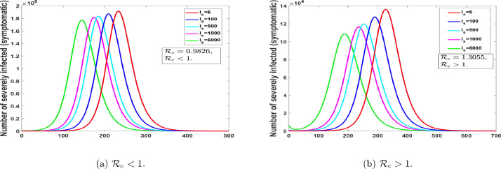
The ramification of Theorem 2.1 is that a small inflow of infectious individuals in the total population will not result in an outbreak if ${\mathcal{R}}_c<1$ [16]. That is the disease will eventually leave the population (when ${\mathcal{R}}_c<1$) suppose the initial data of the infectious people lies in the catchment area of the disease-free equilibrium [16]. The epidemiological ramification of Theorem 2.2 is that the eradication of COVID-19 is not dependent on the initial size of the population [16]. Thus, the initial data of the infectious people do not have to lie in the catchment area of the disease-free equilibrium [16]. Now concerning the model (1), thus, an epidemic model without birth/deaths, the disease always die out, irrespective of Theorem 2.1 and Theorem 2.2, see Fig. 3. Hence, we did not show the mathematical proof of Theorem 2.1 and Theorem 2.2 in this work.

Fig. 3.

An epidemic model without birth/deaths, the disease always dies out, irrespective of Theorem 2.1 and Theorem 2.2.

Remark 1

Using the ideas from [16], we notice the significance of the protective class $S_p$. From the notion of incidence ratio, thus $\frac{S^{*}}{N^{*}}$ gives $\frac{S^{*}}{N^{*}}=\frac{S^{*}}{S^{*}+S_P^{*}}=\frac{N\left(0\right)-S_p^{*}}{N\left(0\right)}=[1-\left(\frac{\alpha }{\omega }\right)]=\frac{S_P^{*}}{N^{*}}\le 1$ is the proportion of protective individuals. Hence, replacing $\frac{S^{*}}{N^{*}}$ by $(1-\frac{\alpha }{\omega })$ shows that the value of ${\mathcal{R}}_c^{*},$ ${\mathcal{R}}_{ec}$ reduces as the value of $\frac{\alpha }{\omega }$ increases, and ${\mathcal{R}}_c^{*},{\mathcal{R}}_{ec}$ increases as the value of $\frac{\alpha }{\omega }$ decreases. Hence, the higher the proportion of individuals in the protective susceptible class the higher the chance of eliminating the second or multiple wave(s) of the disease in Ghana and Egypt.

3. Parameter estimations and Numerical results

To estimate the basic reproduction number and the associated parameter values typically require an indirect method, due to the difficulties in obtaining all parameter values directly from the epidemic data [21]. The most commonly used method is to fit the model to some epidemiological data [21], which provides the minimized estimates of the needed parameters [22]. Model parameters can be obtained by the use of least-square fitting. Thus, the model solution is fitted to the epidemic data [22]. Here, we employ the least square method to the proposed model to obtain the best-fit parameters for Ghana and Egypt using the standard incidence rate. The procedure looks for the set of initial guesses and pre-estimated parameters $\Theta$ for the model whose solutions best fit or pass through all the data points [22], [23], by reducing the sum of the square difference between the observed data $x_t$ and the model solution $K(t,\Theta )$ [22], such that

$$Y\left(\Theta \right)=\sum _{t=1}^n{(x_t-K(t,\Theta ))}^2.$$

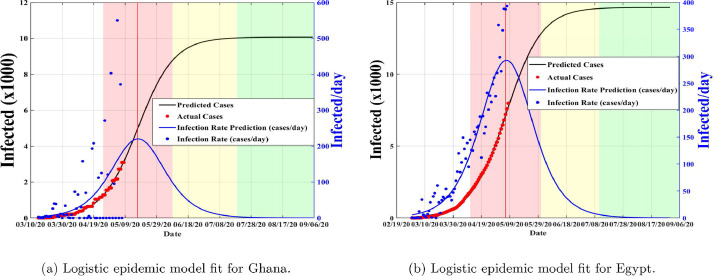
The data used was taken from the Center for System Science and Engineering at Johns Hopkins University and can be found at [24]. The population for Ghana and Egypt were obtained from the worldometer.info [4]. In literature, it is estimated that, the incubation period is from $\frac{1}{5.2}$ to $\frac{1}{3}$ [25], [26], [27], so we set the initial guess to $\rho =\gamma =\frac{1}{5.2}$ and $\sigma =\frac{1}{3}$ for both countries. Also, from literature the proportion of infectious with timely diagnosis is estimated to be (0.3,0.65) in China [27]. Thus, we set our initial guess to $f=0.2$ for both countries. The initial conditions chosen for $R\left(t\right),D\left(t\right),R^A\left(t\right),$ and $S_p\left(t\right)$ are $R\left(0\right)=D\left(0\right)=R^A\left(0\right)=S_p\left(0\right)=0,$ the initial hospitalized (and or isolated cases) is taken to be the number of reported cases at time $t_0.$ The number of initial asymptomatic and exposed are assumed to be equal to the number of initial confirmed cases for both countries. Finally, we assume the initial severely infected individuals yet to be diagnosed for Ghana to be equal to the number of reported cases at time $t_0,$ and that of Egypt to be equal to the number of confirmed cases at time $t_0.$ Using the logistic fit, we obtained the initial epidemic rate per day as $8.754380\times {10}^{-2},$ and $7.987195\times {10}^{-2}$ for Ghana and Egypt respectively as of May 7, 2020. These values are then used as initial transmission rate guesses for the proposed model (1) (see Fig.s 4 (a) and 4(b) for the logistic fit).

Fig. 4.

Predictive logistic model fit for COVID-19 reflecting real data from Ghana and Egypt taken from [24]. Red: fast growth phase, yellow: transition to steady-state phase, green: ending phase [28].

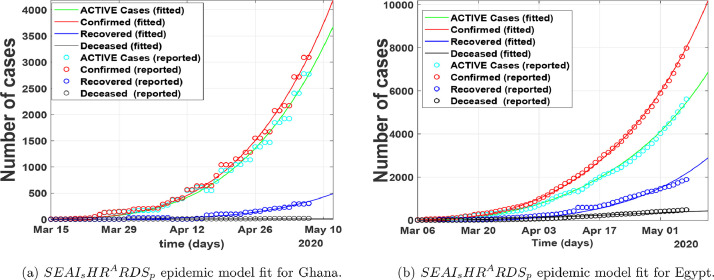
In Fig. 5 , we fitted the proposed COVID-19 model to the epidemic data from March 15, 2020, to May 7, 2020, for Ghana, and March 6, 2020, to May 7, 2020, for Egypt. The red line corresponds to compartment $H$ in the model (1), the red circled corresponds to the real data from Johns Hopkins University [24]. The green circled and the line represents the cumulative active cases respectively. Fig. 5 show that our model relatively fit well to the reported data points.

Fig. 5.

Number of cases per day.

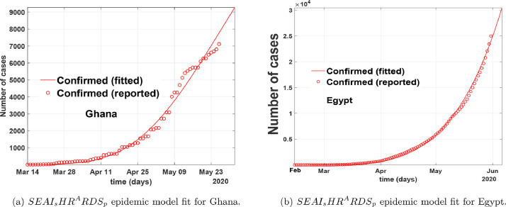
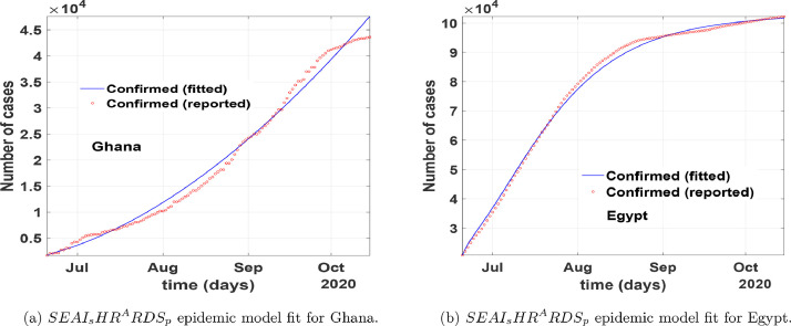
In Fig. 6 , we fitted the proposed COVID-19 model to the epidemic data from the onset of the first recorded cases to the end of May for both Ghana and Egypt by focusing on the number of confirmed cases. The red line corresponds to compartment $H$ in the model (1), the red circled corresponds to the real data from Johns Hopkins University [24]. Fig. 6 show that our model relatively fit well to the reported data points when time is increased and backdated. In Fig. 7 , we fitted the proposed COVID-19 model to the epidemic data from July 01, 2020, to October 31, 2020, for both Ghana and Egypt by focusing on the number of confirmed cases. From Fig. 5-7, we show that our model relatively depicts the COVID-19 real data and control measures implemented in the aforementioned countries within the period March to October 2020, for Ghana, and February to October 2020, for Egypt. From these fittings, the parameter estimates are given in Table 1 . We obtain the control reproduction number, ${\mathcal{R}}_c=1.23$ for Egypt, and ${\mathcal{R}}_c=1.02$ for Ghana, thus assuming the entire population is susceptible.

Fig. 6.

Model fitting of COVID-19 data to $SEA{I}_{s}H{R}^{A}RD{S}_p$ epidemic model from March 12, 2020 to May 31, 2020 for Ghana, and February 14, 2020 to May 31, 2020 for Egypt.

Fig. 7.

Model fitting of COVID-19 data to $SEA{I}_{s}H{R}^{A}RD{S}_p$ epidemic model from July 1, 2020, to October 31, 2020, for Ghana, and Egypt.

Table 1.

Model parameter estimates for our proposed model (1). Since the exact mode of transmission for SARS-CoV-2 is still under effective investigation, these parameters are subject to change and variations as time traverse.

Parameter	Definition	Range	Ghana	Egypt	Source
$\alpha$	Transition rate from the $S$ to the $S_p$ class per day	0.0333 – 0.0677	0.0333	0.0339	Fitted
$\omega$	Transition rate from the $S_p$ to the $S$ class per day	$1.6945\times {10}^{-5}$ – 0.500	$1.6945\times {10}^{-5}$	0.0020	Fitted
$\beta$	Transmission rate from the infectious classes to the $S$ class per day	0.5250 – 0.9250	0.5250	0.6920	Fitted
$q=(1-{\beta }_1)$	Reduced transmission rate from the infectious classes to the $S_p$ class per day	0.0048 – 0.2180	0.0048	0.0182	Fitted
${\eta }_0$	Relative transmissibility in the first incubation phase ($E$ class)	0.0664 – 0.0629	0.0664	0.0629	Fitted
${\eta }_1$	Relative transmissibility in the second incubation phase (asymptomatic individuals) dimensionless	0.5713 – 0.6776	0.5713	0.5776	Fitted
${\eta }_2$	Relative transmissibility of hospitalized individuals	0.4463 – 0.600	0.5642	0.4463	Fitted
$f$	The proportion of individuals from exposure to symptomatic	0.0268 - 0.0648	0.0268	0.0522	Fitted
$(1-f)\rho$	Progression from exposed to asymptomatic	$(1-0.0648)\times 0.1763-(1-0.0310)\times 0.1923$	$(1-0.0268)\times 0.1849$	$(1-0.0522)\times 0.1733$	Fitted
$\gamma$	Progression from exposed to severely infected per day	0.0714 – 0.1923	0.1923	0.1923	[27]
$\sigma$	Rate of progression from asymptomatic to severely infected	0.0025 – 0.1923	0.0025	0.0408	Fitted
$\delta$	Rate of progression from severely infected to hospitalized (or Isolated) per day	0.1264 – 0.5534	0.1264	0.5114	Fitted
$\nu$	Rate of progression from quarantine to hospitalized (or Isolated)	0.1518 – 0.3861	0.1518	0.2847	Fitted
$\tau$	Rate of quarantine	variable	0.1706	0.2	Fitted
$\varphi$	Rate of natural recovery from the asymptomatic stage per day	0.3309 – 0.3256	0.3309	0.3209	Fitted
$r$	Rate of recovery	0.1510 – 0.2229	0.0714	0.2229	Fitted
$k$	Rate of death from $H$	0.0102 – 0.0533	0.0102	0.0533	Estimated
$d$	Rate of death from $I_s$	0.0099 – 0.0500	0.0048	0.0425	Fitted

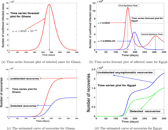
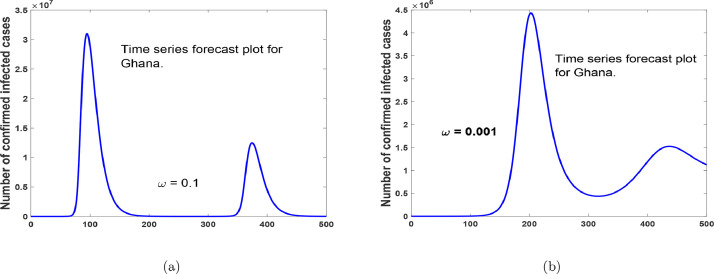
In Fig. 8 , we simulated model (1) using the estimated parameters in Table 1, to depict the populations trajectories. Fig.s 8(a) and 8(b) show the projected peaks for both countries, we see that Ghana has only one peak, thus when the reluctant behaviour on the use of protective equipment is minimized. Which suggest that the second wave of the disease can be stopped if the measures used in curbing the disease are maintained. Alternatively, in Fig. 9 we show that an increase in the reluctant behaviour on the use of protective equipment will lead to a second wave of the COVID-19 in Ghana. In Fig. 8(b) we noticed that there could be a second wave of the disease in Egypt, but this can be avoided if stringent use of protective equipment is implemented for a long time or the reluctant behaviour on the use of protective equipment is minimized as depicted by the blue line. Fig.s 8(c) and 8(d) foretell the projected trajectory of the number of recoveries from the disease in Ghana and Egypt, indicating a continuous raise in recovery in the number of detected and undetected cases respectively, with the number of undetected cases over-seeding that of detected cases.

Fig. 8.

Model-predicted time series of the number of infected cases and recoveries.

Fig. 9.

Time series forecast plot for Ghana, with an increase in reluctant behaviour on the use of protective equipment.

4. Sensitivity analysis

Now, we apply the concept of sensitivity analysis to obtain the relative importance of each model parameter in the control reproduction number, ${\mathcal{R}}_c,$ for the countries Ghana and Egypt, using the fitted values in Table 1. In the present case, the focus is to determine how changes in the model parameters impact the effective reproduction number [29]. This is done through the normalized forward-sensitivity index, Latin hypercube sampling and the partial rank correlation coefficients (PRCC) [29]. Mathematically, the ability to reduce a disease transmission is directly linked to the basic/control reproduction number ${\mathcal{R}}_C,$ and the prevalence of the disease is linked to the endemic equilibrium point [29], [30]. Thus, knowing the relative importance of the various parameters in the basic/control reproduction number helps in determining which strategies should be used to combat the spread of the disease.

Following [29], the normalized forward sensitivity index of ${\mathcal{R}}_c$ with respect to parameter $p_i$ is defined as

$${\Lambda }_{p_i}^{{\mathcal{R}}_c}=\frac{\partial {\mathcal{R}}_c}{\partial p_i}\times \frac{p_i}{{\mathcal{R}}_c}.$$ (5)

Using the parameters values in Table 1, we obtain the sensitivity indices for the two countries as presented in Table 2 . From Table 2, it is clear that, the following parameters $(\beta ,{\beta }_1,{\eta }_0,{\eta }_1,{\eta }_2,f,\gamma ,\rho ,\sigma )$ influence the control reproduction number positively. Thus, a relative increase in these parameters will have a relative index increase in the control reproduction number. Among these parameters, we notice that, the transmission rate $\beta ,$ the relative transmissibility, ${\eta }_1,$ of asymptomatic individuals has the highest impact on ${\mathcal{R}}_c$.

Table 2.

Sensitivity signs of ${\mathcal{R}}_c$ to the parameters in Eq. (2).

Parameter	Ghana (sensitivity index)	Egypt (sensitivity index)
$\beta$	+1.0000	+1.0000
$q=(1-{\beta }_1)$	+0.0068	+0.0179
${\eta }_0$	+0.1861	+ 0.2067
${\eta }_1$	+ 0.5718	+ 0.5552
${\eta }_2$	+ 0.1129	+0.1077
$\gamma$	+0.1785	+0.0512
$f$	+0.1785	+0.0512
$\rho$	-0.3646	-0.2579
$(1-f)$	-0.3646	-0.2579
$\sigma$	+ 0.0327	+ 0.0796
$\delta$	-0.1203	-0.1121
$\tau$	-0.2056	-0.2437
$\varphi$	-0.3989	-0.3910
$r$	-0.0988	-0.0869
$\kappa$	-0.0141	-0.0208
$d$	-0.0092	-0.0142

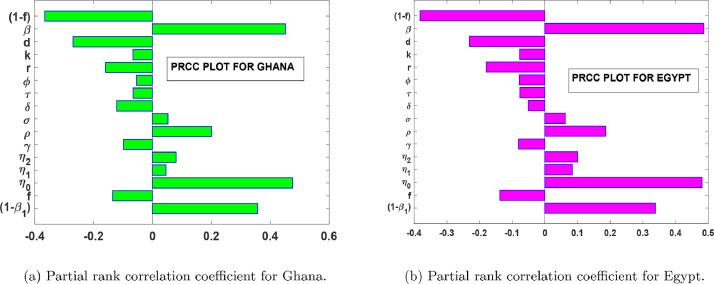
Fig.s 10 (a) and 10(b) shows the global sensitivity analysis of the parameters in the control reproduction number ${\mathcal{R}}_c,$ with a sample size of 2500 runs for both countries. Averagely, we noticed from the Tornado plots in Fig.s 10(a) and 10(b) that, any positive perturbation in the parameters $(\beta ,\rho ,\gamma ,{\eta }_0,{\eta }_1,{\eta }_2,\sigma ,{\beta }_1,f)$ will have a corresponding percentage increase in the severity of the disease in both countries. We also noticed from Fig.s 10(a) and 10(b) that, the most influential parameters that affect ${\mathcal{R}}_c$ positively are: $\beta ,$ ${\eta }_0,$ and $(1-{\beta }_1).$ Thus, measures such as the washing of hands, wearing of an effective nose mask, the use of effective personal protective equipment in the hospitals or the isolation centres, and the continuous advocacy on prevention measures through the media and adhering to social distancing will help reduce the intensity of $\beta ,$ ${\eta }_0,$ and $(1-{\beta }_1).$ Furthermore, in Table 2, it shows that the control reproduction number, ${\mathcal{R}}_c,$ can be reduced through an increase in the values of $(\delta ,\tau ,r,k,d,\varphi ).$ But, since $k$ and $d$ represent death rates, we cannot use them as a control measure, therefore, we can strengthen the remaining four parameters $(\delta ,\tau ,r,\varphi )$ so as to reduce the number of infections. Thus, the increase in the timely diagnosis of infected individuals, increase in contact tracing, managing of detected cases and consumption of foods that boost the immune system and/or healthy lifestyle practices (such as avoiding smoking) will help reduce the severity of the disease.

Fig. 10.

PRCC plots for parameters in ${\mathcal{R}}_c$.

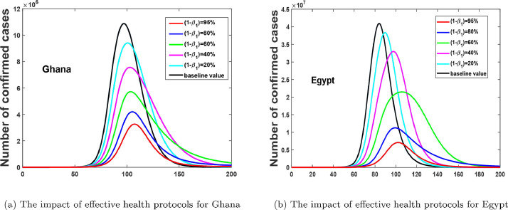
From the PCCR plots in Fig. 10, we notice that, $\beta ,$ ${\eta }_0,$ $(1-{\beta }_1),$ and $\rho$ are the most influential parameters on ${\mathcal{R}}_c$; and that, its control will reduce the rate of secondary infections. Therefore, in Fig. 11 (a) and 11(b), we show the positive impact of health protocols (lockdowns, facemasks, PPE, hygiene, physical distancing, etc, i.e. all non-pharmaceutical interventions apart from case isolation) for both countries. Fig. 11(a) and 11(b), depicts that, an increase in the effectiveness of protective materials or health protocols will reduce the number of confirmed cases.

Fig. 11.

Effect of varying the impact of $(1-{\beta }_1)$ health protocols.

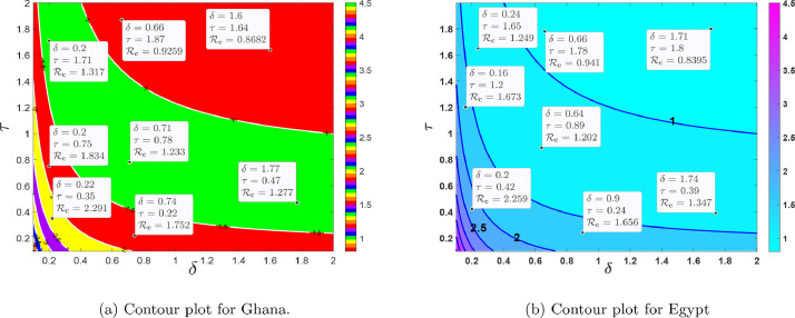
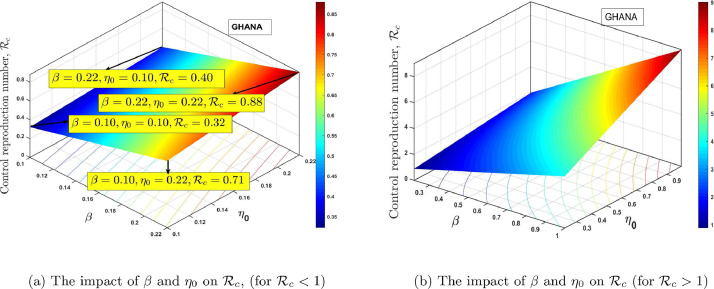
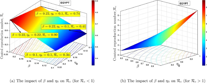
Fig. 12 (a) and 12(b), shows the contour plot of the control reproduction number ${\mathcal{R}}_c,$ as a function of diagnosis parameter $\left(\delta \right),$ and effective quarantine of asymptomatic individuals through contact tracing for Ghana and Egypt respectively. This indicates that to effectively reduce the control reproduction number to less than a unity requires effective non-pharmaceutical interventions such as the strict use of nose mask and face shields in public, media education campaigns on preventive measures, physical distancing, and doubling enhanced contact-tracing. From the PRCC plots in Fig. 10, we notice that, $\beta ,$ ${\eta }_0,$ $(1-{\beta }_1),$ and $\rho$ are the most influential parameters on ${\mathcal{R}}_c,$ and that, its control will reduce the rate of secondary infections. The estimated proportion of individuals who become severely infected from the exposed class based on the model (1) is estimated to be approximately 2.7% and 5.2% for Ghana and Egypt respectively, which implies that the percentage of asymptomatic individuals who get the disease without knowing is approximately 97.30% and 95.80% respectively, this reinforces the need for more effective contact tracing and testing in both countries. In Fig. 13 (a) and 14 (a), we show the impact of having a low transmissivity rate of exposed individuals to the susceptible individuals, which can be achieved by the washing of hands with soap, cleaning of doorknobs and surfaces, etc. In parameter terms, it indicates that, a range of values of $(0.1-0.2)$ for both $\beta$ and ${\eta }_0$ will peak the control reproduction number, ${\mathcal{R}}_c$ in the range $(0.1-0.88)$ for Ghana and $(0.2-0.95)$ for Egypt. In Fig.s 13(b) and 14(b), we show the impact of high values of $\beta$ and ${\eta }_0$ on the proposed model and the computed control reproduction number, ${\mathcal{R}}_c$. It indicates that any possible combination of the parameter values in Table 1, together with the following range of values, $[0.22-1]$ for $\beta$ and ${\eta }_0$ will produce high control reproduction number.

Fig. 12.

The dynamical effect of timely diagnoses and effective quarantine.

Fig. 13.

Effect of varying the values of the transmission rate, $\beta ,$ and the transmissibility rate of the exposed class, ${\eta }_0$.

Fig. 14.

Effect of varying the values of transmission rate, $\beta ,$ and transmissibility rate of the exposed class, ${\eta }_0$.

5. Optimal control model and analysis

5.1. Non-autonomous version of model (1)

Now, we update the model (1) based on the sensitivity analysis results in Section 4 to study the effects of optimal health protocols-personal protections (thus, physical distancing, media advocacy, wearing of a nose mask, the use of hand sanitiser-washing of hands, lockdowns, stringent safety measures in hospitals (and/or isolation centres), with a constant supply of effective personal protective equipment (PPE)), testing-diagnoses and contact tracing. Thus, we seek to determine the optimal trajectories which depict the effects of these controls. To determine the optimal trajectories strategies, we let $u_1\left(t\right)$ to represent health protocols-personal protections (thus, physical distancing, media advocacy, wearing of a nose mask, the use of hand sanitiser-washing of hands, lockdowns, stringent safety measures in hospitals (and/or isolation centres), with a constant supply of effective personal protective equipment (PPE)), while $u_2\left(t\right)$ denotes contact tracing (testing-diagnoses). Thus, the two control variables are incorporated into the autonomous system (1) such that the disease transmission terms in model (1) are reduced by the factor $[1-u_1\left(t\right)]$ while the rate of contact tracing (testing-diagnoses) of asymptomatic infected individuals for quarantine, $\tau ,$ is modified as $u_2\tau$. Hence, the optimal control model corresponding to the adjusted model (1) is expressed by the model (6) as

$$\begin{array}{c}\frac{dS}{dt}=-(1-u_1)\beta \frac{({\eta }_{0}E+{\eta }_{1}A+I_s+{\eta }_{2}H)S}{N-Q-D}-\alpha S+\omega S_p,\hfill \\ \frac{dE}{dt}=(1-u_1)\beta \frac{({\eta }_{0}E+{\eta }_{1}A+I_s+{\eta }_{2}H)S}{N-Q-D}\hfill \\ +(1-{\beta }_1)(1-u_1)\beta \frac{({\eta }_{0}E+{\eta }_{1}A+I_s+{\eta }_{2}H)S_p}{N-Q-D}-(1-f)\rho E-f\gamma E,\hfill \\ \frac{dA}{dt}=(1-f)\rho E-u_2\tau A-\sigma A-\varphi A,\hfill \\ \frac{dQ}{dt}=u_2\tau A-\nu Q,\hfill \\ \frac{d{R}^A}{dt}=\varphi A,\hfill \\ \frac{dR}{dt}=rH,\hfill \\ \frac{d{I}_s}{dt}=f\gamma E+\sigma A-(\delta +d)I_s,\hfill \\ \frac{dH}{dt}=\nu Q+\delta I_s-rH-\kappa H,\hfill \\ \frac{dD}{dt}=\kappa H,\hfill \\ \frac{d{S}_p}{dt}=\alpha S-\omega S_p-(1-u_1)\beta \frac{({\eta }_{0}E+{\eta }_{1}A+I_s+{\eta }_{2}H)S}{N-Q-D},\hfill \end{array}$$ (6)

subject to suitable initial conditions at time $t=0$.

5.2. Objective functional

Our goal is to minimize the numbers of infected (including the exposed, asymptomatic, symptomatic and hospitalized) individuals along with the costs of implementing health protocols-personal protections and contact-tracing (testing-diagnoses) controls simultaneously. Thus, the mathematical setup of the optimal control problem includes the minimization of an objective functional $J$ given as

$$J[u_1,u_2]={\int }_0^{t_k}[W_{1}E+W_{2}A+W_3{I}_s+W_{4}H+\frac{C_1{u}_1^2\left(t\right)}{2}+\frac{C_2{u}_2^2\left(t\right)}{2}]dt$$ (7)

constrained by the system (6), where the positive balancing constants $W_i>0,i=1,2,3,4$ and $C_1,C_2>0$ are correctly taken. The coefficients, $W_1>0,W_2>0,W_3>0,W_4>0$ are introduced to keep the balance of the cost size of reducing the disease transmission, $C_1$ and $C_2$ are the corresponding weights associated with the cost of the control measures $u_1$ and $u_2,$ with $C_1$ being the cost associated with health protocols-personal protections and $C_2$ is the cost associated with contact tracing (testing-diagnoses). The final time for the implementation of the two controls is denoted $t_k$. The nonlinearities with the cost of controls are taken care of by the square terms in the objective functional (7) and the half terms normalize the cost associated with our chosen controls [31], [32], [33]. Further, the total cost $\left(\mathcal{TC}\right)$ for the proposed optimal control is defined as

$$\mathcal{TC}={\int }_0^{t_k}\frac{1}{2}\sum _{i=1}^2{C}_i{u}_i^2\left(t\right)dt,$$ (8)

where $C_1,C_2>0,$ are the hypothetical unit cost of the control interventions. Our interest, in particular, is to seek an optimal control $u^{*}=(u_1^{*},u_2^{*})$ such that

$$J\left(u^{*}\right)=\min \{J(u_1,u_2):u_1,u_2\in U\}$$ (9)

where, $U$ is an admissible control set $U,$ which is Lebesgue measurable and defined as

$$U=\{\left(u_i\right)\left(t\right)\mid 0\le u_i\left(t\right)\le u_{i\max }\left(t\right)\le 1,t\in [0,t_k],i=1,2\}.$$ (10)

5.3. Existence and characterization of optimal controls

Theorem 5.1

Given an optimal control $u^{*}=(u_1^{*},u_2^{*})\in U$ exists for model (6) then

$$J(u_1^{*},u_2^{*})=\underset{(u_1,u_2)\in U}{\min }J(u_1,u_2).$$

Proof

Using the Fleming and Rishel ([34], Theorem 4.1, 68-69), the existence of the proposed optimal control is an outcome of the convexity of the integrand of $J$ with respect to $u_1,$ and $u_2,$ a priori boundedness of the state variables, and the Lipschitz property of the state system with respect to the state variables [35], [36], [37], [38]. The compactness required for the existence of control problem is obtained from the boundedness of the optimal system. Furthermore, the term $W_{1}E+W_{2}A+W_3{I}_s+W_{4}H+\frac{C_1{u}_1^2\left(t\right)}{2}+\frac{C_2{u}_2^2\left(t\right)}{2}$ in Eq. (7) is convex on the control set $U$. Hence, we can now state that there is a positive constant ${\eta }^{*}>1$ and nonnegative constants $v_1>0,v_2>0$ such that

$$J(u_1,u_2)\ge v_1{\left(|u_1{|}^2+|u_2{|}^2\right)}^{\frac{{\eta }^{*}}{2}}-v_2,$$

this leads to the existence of the optimal control problem [39], [40]. □

5.3.1. Characterization of optimal controls

Employing the Pontryagin's maximum principle (PMP), model (6) and the objective functional (7) is converted into a pointwise Hamiltonian, $\mathcal{H},$ with respect to $(u_1,u_2)$. Thus,

$$\begin{array}{ccc}\hfill \mathcal{H}& =& W_{1}E+W_{2}A+W_3{I}_s+W_{4}H+\frac{C_1{u}_1^2}{2}+\frac{C_2{u}_2^2}{2}\hfill \\ & & +{\lambda }_S[-(1-u_1)\beta \frac{({\eta }_{0}E+{\eta }_{1}A+I_s+{\eta }_{2}H)S}{N-Q-D}-\alpha S+\omega S_p]\hfill \\ & & +{\lambda }_E\left[(1-u_1)\beta \frac{({\eta }_{0}E+{\eta }_{1}A+I_s+{\eta }_{2}H)S}{N-Q-D}\right]\hfill \\ & & +{\lambda }_E\left[(1-{\beta }_1)(1-u_1)\beta \frac{({\eta }_{0}E+{\eta }_{1}A+I_s+{\eta }_{2}H)S_p}{N-Q-D}\right]\hfill \\ & & +{\lambda }_E[-(1-f)\rho E-f\gamma E]\hfill \\ & & +{\lambda }_A[(1-f)\rho E-u_2\tau A-\sigma A-\varphi A]+{\lambda }_Q[u_2\tau A-\nu Q]\hfill \\ & & +{\lambda }_{I_s}[f\gamma E+\sigma A-(\delta +d)I_s]\hfill \\ & & +{\lambda }_H[\nu Q+\delta I_s-\mathit{rH}-\kappa H]+{\lambda }_{R^A}\left[\varphi A\right]+{\lambda }_R\left[\mathit{rH}\right]+{\lambda }_D\left[\kappa H\right]\hfill \\ & & +{\lambda }_{S_p}[\alpha S-\omega S_p-(1-u_1)\beta \frac{({\eta }_{0}E+{\eta }_{1}A+I_s+{\eta }_{2}H)S}{N-Q-D}],\hfill \end{array}$$ (11)

where ${\lambda }_S,{\lambda }_E,{\lambda }_A,{\lambda }_Q,{\lambda }_{I_s},$ ${\lambda }_H,{\lambda }_{R^A},{\lambda }_R,{\lambda }_D,{\lambda }_{S_p}$ are the adjoint variables or co-state variables associated with the state variables $S,S_p,A,I_s,Q,H,D,R^A,R$. Then, the necessary conditions for the optimal control $u^{*}=(u_1^{*},u_2^{*})$ is summarized in Theorem 5.2.

Theorem 5.2

Given the optimal controls$(u_1,u_2)=(u_1^{*},u_2^{*})$and corresponding solutions

$S,S_p,A,I_s,Q,H,R^A,R=S^{\diamond },S_p^{\diamond },A^{\diamond },I_s^{\diamond },Q^{\diamond },H^{\diamond },D^{\diamond }{R^A}^{\diamond },R^{\diamond }$of model(6)that minimizes$J(u_1^{*},u_2^{*})$over$U$. Then there exists co-state variables or adjoint variables,${\lambda }_S,{\lambda }_E,{\lambda }_A,{\lambda }_Q,{\lambda }_{I_s},$${\lambda }_H,{\lambda }_{R^A},{\lambda }_R,{\lambda }_D,{\lambda }_{S_p}$that satisfies

$$\frac{d{\lambda }_j}{dt}=-\frac{\partial \mathcal{H}}{\partial j},$$ (12)

with transversality conditions

$${\lambda }_j\left(T\right)=0,\text{where}j=({\lambda }_S,{\lambda }_E,{\lambda }_A,{\lambda }_Q,{\lambda }_{I_s},{\lambda }_H,{\lambda }_{R^A},{\lambda }_R,{\lambda }_D,{\lambda }_{S_p}).$$

Then the optimality conditions that minimize the Hamiltonian,$\mathcal{H}$, of equation(11)with respect to the controls is

$$\frac{\partial \mathcal{H}}{\partial u_i}=0,i=1,2$$

in the domain of the control set$U$. Hence, these controls are characterized by

$$\begin{array}{ccc}\hfill u_1^{*}& =& \min \{\max \{0,\frac{\frac{S^{\diamond }\beta (I_s^{\diamond }+A^{\diamond }{\eta }_1+E^{\diamond }{\eta }_0+H^{\diamond }{\eta }_2)}{N^{\diamond }-Q^{\diamond }-D^{\diamond }}(({\lambda }_E-{\lambda }_S)+({\lambda }_E-{\lambda }_{S_p}))}{C_1}\},u_{1\max }\},\hfill \\ \hfill u_2^{*}& =& \min \{\max \{0,\frac{\tau A^{\diamond }({\lambda }_A-{\lambda }_Q)}{C_2}\},u_{2\max }\}.\hfill \end{array}$$ (13)

The results in(13)indicate that the controls are bounded with lower bounds zeros and upper bounds$u_{1\max }=1,$$u_{2\max }=1,$such that

$$\begin{array}{ccc}\hfill u_1& =& \{\begin{array}{cc}0\hfill & \text{if}\left({▵}^{*}\right)\le 0,\hfill \\ \left({\Delta }^{*}\right)\hfill & \text{if}0<\left({▵}^{*}\right)<u_{1\max },\hfill \\ u_{1\max }\hfill & \text{if}\left({▵}^{*}\right)\ge u_{1\max },\hfill \end{array}\hfill \\ \hfill u_2& =& \{\begin{array}{cc}0\hfill & \text{if}\frac{\tau A^{\diamond }({\lambda }_A-{\lambda }_Q)}{C_2}\le 0,\hfill \\ \frac{\tau A^{\diamond }({\lambda }_A-{\lambda }_Q)}{C_2}\le 0,\hfill & \text{if}0<\frac{\tau A^{\diamond }({\lambda }_A-{\lambda }_Q)}{C_2}<u_{2\max },\hfill \\ u_{2\max }\hfill & \text{if}\frac{\tau A^{\diamond }({\lambda }_A-{\lambda }_Q)}{C_2}\ge u_{2\max },\hfill \end{array}\hfill \end{array}$$

where

$${▵}^{*}=\frac{\frac{S^{\diamond }\beta (I_s^{\diamond }+A^{\diamond }{\eta }_1+E^{\diamond }{\eta }_0+H^{\diamond }{\eta }_2)}{N^{\diamond }-Q^{\diamond }-D^{\diamond }}(({\lambda }_E-{\lambda }_S)+({\lambda }_E-{\lambda }_{S_p}))}{C_1}.$$

Proof

Taking the partial derivatives of the Hamiltonian $\mathcal{H},$ with respect to the associated state variable we obtain the following adjoint system, which reflect (12).

$$\begin{array}{cc}\frac{d{\lambda }_S}{\mathit{dt}}=\hfill & {\lambda }_S(\alpha +\frac{\beta (u_1-1)(I_s^{\diamond }+A^{\diamond }{\eta }_1+E^{\diamond }{\eta }_0+H^{\diamond }{\eta }_2)}{D^{\diamond }-N^{\diamond }+Q^{\diamond }})\hfill \\ & -{\lambda }_{S_p}(\alpha -\frac{\beta (u_1-1)(I_s^{\diamond }+A^{\diamond }{\eta }_1+E^{\diamond }{\eta }_0+H^{\diamond }{\eta }_2)}{D^{\diamond }-N^{\diamond }+Q^{\diamond }})\hfill \\ & -\frac{\beta {\lambda }_E(u_1-1)(I_s^{\diamond }+A^{\diamond }{\eta }_1+E^{\diamond }{\eta }_0+H^{\diamond }{\eta }_2)}{D^{\diamond }-N^{\diamond }+Q^{\diamond }},\hfill \\ \frac{d{\lambda }_E}{\mathit{dt}}=\hfill & {\lambda }_E(f\gamma -\rho (f-1)-\frac{S^{\diamond }\beta {\eta }_0(u_1-1)}{D^{\diamond }-N^{\diamond }+Q^{\diamond }})\hfill \\ & +{\lambda }_E\left(\frac{S_p^{\diamond }\beta {\eta }_0({\beta }_1-1)(u_1-1)}{D^{\diamond }-N^{\diamond }+Q^{\diamond }}\right)\hfill \\ & -W_1-f\gamma {\lambda }_{I_s}+{\lambda }_A\rho (f-1)+\frac{S^{\diamond }\beta {\eta }_0{\lambda }_S(u_1-1)}{D^{\diamond }-N^{\diamond }+Q^{\diamond }}\hfill \\ & +\frac{S^{\diamond }\beta {\eta }_0{\lambda }_{S_p}(u_1-1)}{D^{\diamond }-N^{\diamond }+Q^{\diamond }},\hfill \\ \frac{d{\lambda }_A}{\mathit{dt}}=\hfill & {\lambda }_A(\varphi +\sigma +\tau u_2)-{\lambda }_{R^A}\varphi -{\lambda }_{I_s}\sigma -W_2\hfill \\ & -{\lambda }_E(\frac{S^{\diamond }\beta {\eta }_1(u_1-1)}{D^{\diamond }-N^{\diamond }+Q^{\diamond }}-\frac{S_p^{\diamond }\beta {\eta }_1({\beta }_1-1)(u_1-1)}{D^{\diamond }-N^{\diamond }+Q^{\diamond }})\hfill \\ & -{\lambda }_Q\tau u_2+\frac{S^{\diamond }\beta {\eta }_1{\lambda }_S(u_1-1)}{D^{\diamond }-N^{\diamond }+Q^{\diamond }}+\frac{S^{\diamond }\beta {\eta }_1{\lambda }_{S_p}(u_1-1)}{D^{\diamond }-N^{\diamond }+Q^{\diamond }},\hfill \\ \frac{d{\lambda }_Q}{\mathit{dt}}=\hfill & {\lambda }_Q\nu -{\lambda }_H\nu \hfill \\ & +{\lambda }_E\left(\frac{S^{\diamond }\beta (u_1-1)(I_s^{\diamond }+A^{\diamond }{\eta }_1+E^{\diamond }{\eta }_0+H^{\diamond }{\eta }_2)}{{(D^{\diamond }-N^{\diamond }+Q^{\diamond })}^2}\right)\hfill \\ & +{\lambda }_E(-\frac{S_p^{\diamond }\beta ({\beta }_1-1)(u_1-1)(I_s^{\diamond }+A^{\diamond }{\eta }_1+E^{\diamond }{\eta }_0+H^{\diamond }{\eta }_2)}{{(D^{\diamond }-N^{\diamond }+Q^{\diamond })}^2})\hfill \\ & -\frac{S^{\diamond }\beta {\lambda }_S(u_1-1)(I_s^{\diamond }+A^{\diamond }{\eta }_1+E^{\diamond }{\eta }_0+H^{\diamond }{\eta }_2)}{{(D^{\diamond }-N^{\diamond }+Q^{\diamond })}^2}\hfill \\ & -\frac{S^{\diamond }\beta {\lambda }_{S_p}^{\diamond }(u_1-1)(I_s^{\diamond }+A^{\diamond }{\eta }_1+E^{\diamond }{\eta }_0+H^{\diamond }{\eta }_2)}{{(D^{\diamond }-N^{\diamond }+Q^{\diamond })}^2},\hfill \\ \frac{d{\lambda }_{I_s}}{\mathit{dt}}=\hfill & {\lambda }_{I_s}(d+\delta )-{\lambda }_E(\frac{S^{\diamond }\beta (u_1-1)}{D^{\diamond }-N^{\diamond }+Q^{\diamond }}-\frac{S_p^{\diamond }\beta ({\beta }_1-1)(u_1-1)}{D^{\diamond }-N^{\diamond }+Q^{\diamond }})\hfill \\ & -W_3-\delta {\lambda }_H\hfill \\ & +\frac{S^{\diamond }\beta {\lambda }_S(u_1-1)}{D^{\diamond }-N^{\diamond }+Q^{\diamond }}+\frac{S^{\diamond }\beta {\lambda }_{S_p}(u_1-1)}{D^{\diamond }-N^{\diamond }+Q^{\diamond }},\hfill \\ \frac{d{\lambda }_H}{\mathit{dt}}=\hfill & {\lambda }_H(\kappa +r)-W_4-\kappa {\lambda }_D-{\lambda }_{R}r\hfill \\ & -{\lambda }_E(\frac{S^{\diamond }\beta {\eta }_2(u_1-1)}{D^{\diamond }-N^{\diamond }+Q^{\diamond }}-\frac{S_p^{\diamond }\beta {\eta }_2({\beta }_1-1)(u_1-1)}{D^{\diamond }-N^{\diamond }+Q^{\diamond }})\hfill \\ & +\frac{S^{\diamond }\beta {\eta }_2{\lambda }_S(u_1-1)}{D^{\diamond }-N^{\diamond }+Q^{\diamond }}+\frac{S^{\diamond }\beta {\eta }_2{\lambda }_{S_p}(u_1-1)}{D^{\diamond }-N^{\diamond }+Q^{\diamond }},\hfill \end{array}$$

$$\begin{array}{cc}\frac{d{\lambda }_D}{\mathit{dt}}=\hfill & {\lambda }_E\left(\frac{S^{\diamond }\beta (u_1-1)(I_s^{\diamond }+A^{\diamond }{\eta }_1+E^{\diamond }{\eta }_0+H^{\diamond }{\eta }_2)}{{(D^{\diamond }-N^{\diamond }+Q^{\diamond })}^2}\right)\hfill \\ & -{\lambda }_E\left(\frac{S_p^{\diamond }\beta ({\beta }_1-1)(u_1-1)(I_s^{\diamond }+A^{\diamond }{\eta }_1+E^{\diamond }{\eta }_0+H^{\diamond }{\eta }_2)}{{(D^{\diamond }-N^{\diamond }+Q^{\diamond })}^2}\right)\hfill \\ & -\frac{S^{\diamond }\beta {\lambda }_S(u_1-1)(I_s^{\diamond }+A^{\diamond }{\eta }_1+E^{\diamond }{\eta }_0+H^{\diamond }{\eta }_2)}{{(D^{\diamond }-N^{\diamond }+Q^{\diamond })}^2}\hfill \\ & -\frac{S^{\diamond }\beta {\lambda }_{S_p}(u_1-1)(I_s^{\diamond }+A^{\diamond }{\eta }_1+E^{\diamond }{\eta }_0+H^{\diamond }{\eta }_2)}{{(D^{\diamond }-N^{\diamond }+Q^{\diamond })}^2},\hfill \\ \frac{d{\lambda }_{S_p}}{\mathit{dt}}=\hfill & {\lambda }_{S_p}\omega -{\lambda }_S\omega \hfill \\ & +\frac{\beta {\lambda }_E({\beta }_1-1)(u_1-1)(I_s^{\diamond }+A^{\diamond }{\eta }_1+E^{\diamond }{\eta }_0+H^{\diamond }{\eta }_2)}{D^{\diamond }-N^{\diamond }+Q^{\diamond }}.\hfill \end{array}$$

Also, taking the partial derivatives of $\mathcal{H}$ with respect to the controls gives

$$\begin{array}{c}{\displaystyle \frac{\partial \mathcal{H}}{\partial u_1}}=C_1{u}_1\hfill \\ +{\lambda }_E(\frac{S^{\diamond }\beta (I_s^{\diamond }+A^{\diamond }{\eta }_1+E^{\diamond }{\eta }_0+H^{\diamond }{\eta }_2)}{D^{\diamond }-N^{\diamond }+Q^{\diamond }}-\frac{S_p^{\diamond }\beta ({\beta }_1-1)(I_s^{\diamond }+A^{\diamond }{\eta }_1+E^{\diamond }{\eta }_0+H^{\diamond }{\eta }_2)}{D^{\diamond }-N^{\diamond }+Q^{\diamond }})\hfill \\ -\frac{S^{\diamond }\beta {\lambda }_S(I_s^{\diamond }+A^{\diamond }{\eta }_1+E^{\diamond }{\eta }_0+H^{\diamond }{\eta }_2)}{D^{\diamond }-N^{\diamond }+Q^{\diamond }}-\frac{S^{\diamond }\beta {\lambda }_{S_p}(I_s^{\diamond }+A^{\diamond }{\eta }_1+E^{\diamond }{\eta }_0+H^{\diamond }{\eta }_2)}{D^{\diamond }-N^{\diamond }+Q^{\diamond }}=0,\hfill \\ {\displaystyle \frac{\partial \mathcal{H}}{\partial u_2}}=C_2{u}_2-A^{\diamond }{\lambda }_A\tau +A^{\diamond }{\lambda }_Q\tau =0.\hfill \end{array}$$ (14)

Replacing $u_1=u_1^{*},u_2=u_2^{*}$ into Eq. (14) and solving for $u_i^{*},i=1,2$ respectively leads to the results in Eq. (13), which completes the proof. In the next section, we present the numerical results of the optimality system, the control profile and discussions. □

5.4. Numerical illustration and discussion

In this section, we observe the optimal trajectories of the optimality system. Thus, in doing so we applied the forward-backward sweep method which has been extensively explained by Lenhart and Workman [41]. The constraint system (6) is solved forward in time and the adjoint system is solved backward in time with corresponding lower and upper bounds for the controls, and initial conditions for the state variables. For the simulation we used the following initial conditions, $N\left(0\right)=102334404,\delta =0.05114,d=0.000425,$

$$\begin{array}{ccc}& & \left[N\right(0)-135,100,10,10,15,0,0,0,0,0]\hfill \\ & & =[S\left(0\right),E\left(0\right),A\left(0\right),Q\left(0\right),I\left(0\right),H\left(0\right),R^A\left(0\right),R\left(0\right),D\left(0\right),S_P\left(0\right)],\hfill \end{array}$$

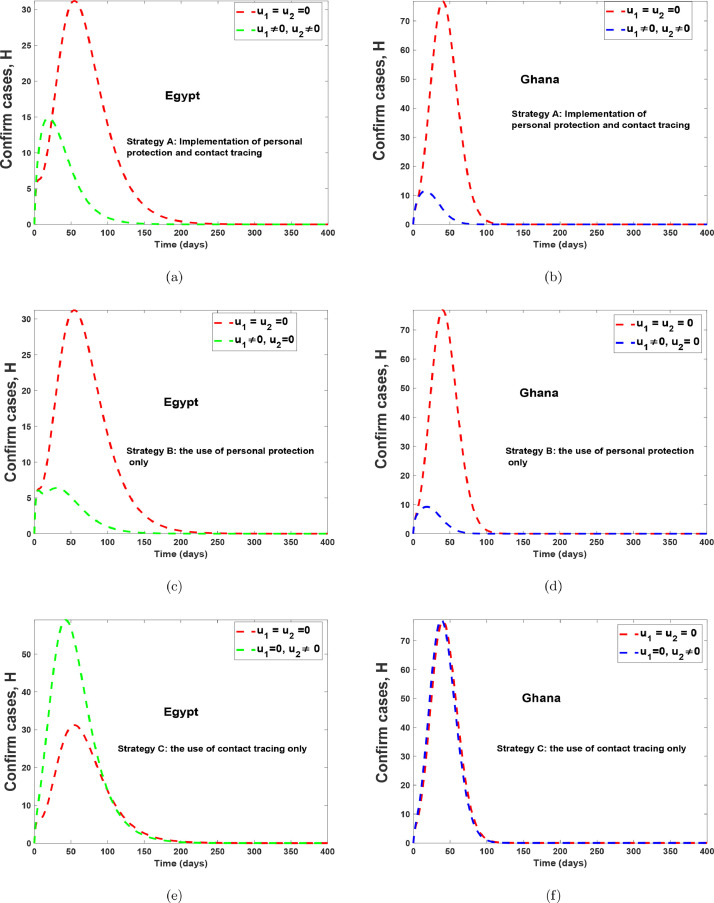
for Egypt, and $N\left(0\right)=31072940,\left[N\right(0)-126,100,10,10,6,0,0,0,0,0],\beta =0.9250,\sigma =0.1025,\delta =0.2126,\nu =0.2118$ for Ghana, together with the other parameters values in Table 1, $N\left(0\right)=\text{Initial}\text{total}\text{population}$. The weight associated with the objective function (7), is hypothetically taken as $W_1=2,W_2=2,W_3=2,W_4=2,$ the cost weight is hypothetically taken as $C_1=\$2.00,C_2=\$2.00,$ and the lower (LB) and upper (UB) bounds is taken as $L{B}_1=0,U{B}_1=1,L{B}_2=0,U{B}_2=1$. The simulations of the optimal control is divided into different strategies to illustrate the diverse impact of considering one or more controls. Thus:

• (i)Strategy A: the implementation of health protocols-personal protections and contact tracing (testing-diagnoses), thus, $(u_1,u_2\ne 0),$
• (ii)Strategy B: the use of health protocols-personal protections only $(u_1\ne 0,u_2=0),$
• (iii)Strategy C: the use of contact tracing (testing-diagnoses) only $(u_1=0,u_2\ne 0)$.

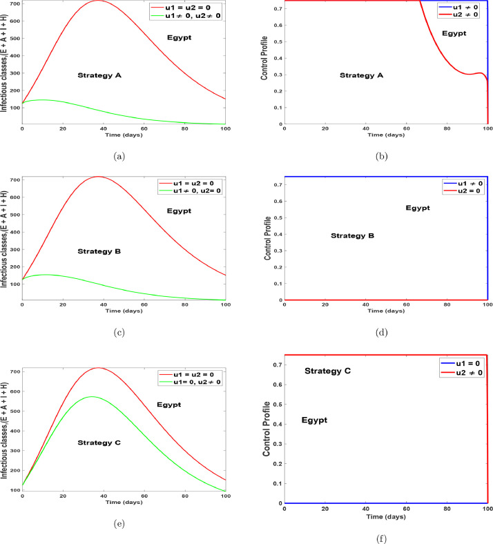
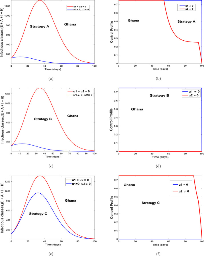
Fig. 15 and 16 shows the implementation of the various controls strategies on the model. It indicates that, the disease in the infectious population can be brought down faster when both controls are implemented as compared to situations without controls or with the use of a single control. The optimal control trajectories from the simulations shows that a proper combination of the control strategies may lead to a desirable control of COVID-19. Fig. 17 (a)-17(b) shows the implementation of strategy A on the number of confirm cases. It indicates that, the confirm population can be eliminated within 120 days for Egypt and within 70 days for Ghana, as compared to situations without controls. Fig. 17(c)-17(d) shows the impact of health protocols-personal protections only on the number of confirm cases. Fig. 17(c)-17(d) equally shows the efficacy of strategy B, which indicates that strategy B is the best alternative control if a country does not implement strategy A. Fig. 17(e)-17(f), indicates that, if one wants to achieve the desired trajectories as depicted in Fig. 17(a)-17(b), then the use of contact tracing (testing-diagnoses) should not be the only control choice by health authorities. The control profiles for Fig. 17, has similar dynamics as that of Fig. 15 and Fig. 16, therefore it is not shown here. The simulations of the optimal control strategies show that a proper combination of the control strategies or a good choice of a single control strategy may lead to a desirable control COVID-19. Nevertheless, it is also important to choose a strategy that gives optimal cost (thus less cost) when these controls are implemented on a large scale. Hence, we study the cost-effectiveness of these controls in the preceding section.

Fig. 15.

Optimal simulation with the implementation of various control strategies for Egypt.

Fig. 16.

Optimal simulation with the implementation of various control strategies for Ghana.

Fig. 17.

Optimal simulation with the implementation of various control strategies for Egypt and Ghana.

6. Cost-effectiveness analysis

To control or eradicate COVID-19 infections in a population can be either labour-intensive or expensive, or even both. For these reasons, it is crucial to conduct a cost-effectiveness analysis. The current section discusses the application of cost-effectiveness analysis to examine the cost-effectiveness related to the use of two time-dependent control functions $u_1\left(t\right)$ and $u_2\left(t\right)$. To this end, we consider three strategies for the use of the two time-dependent control functions $u_1\left(t\right)$ and $u_2\left(t\right)$ as defined in subsection 5.4.

To implement the cost-effectiveness analysis, we use three approaches, namely, the Infection Averted Ratio (IAR), the Average Cost-Effectiveness Ratio (ACER) and the Incremental Cost-Effectiveness Ratio (ICER), as defined in [31], [37], [42], [43], [44], [45]. The three cost-effectiveness approaches are iterated as follows:

Infection Averted Ratio (IAR)

The most effective strategy when using (IAR) is the strategy with the highest ratio. The mathematical representation of the infection averted ratio is defined as:

$$IAR=\frac{\text{Cumulative}\text{infection}\text{averted}}{\text{Cumulative}\text{recoveries}}.$$

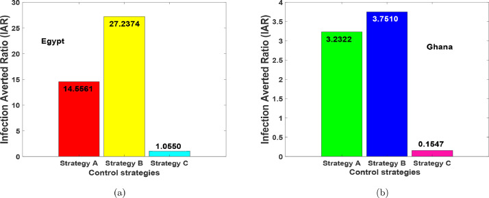
From the parameter values in Table 1, the $IAR$ for the various optimal interventions were obtained. Fig. 18 depicts the $IAR$ for the three optimal strategies. Strategy B containing the implementation of health protocols-personal protections $\left(u_1\left(t\right)\right)$ such as the use of physical distancing, media advocacy, wearing of a nose mask, the use of hand sanitiser-washing of hands, lockdowns, stringent safety measures in hospitals (and/or isolation centres), with a constant supply of effective personal protective equipment (PPE) generates the highest $IAR$ ratio and hence the most effective. This is preceded by Strategy A containing the implementation of health protocols-personal protections measures $\left(u_1\left(t\right)\right)$ and contact tracing (testing-diagnoses) $\left(u_2\left(t\right)\right)$. Strategy C, contact tracing (testing-diagnoses) only shows to be the least effective measure for both countries.

Fig. 18.

Infection Averted Ratio (IAR) results for Strategies A–C.

Average Cost-Effectiveness Ratio

The average cost-effectiveness ratio (ACER) is calculated against the worst cases of no intervention (i.e., $u_1=u_2=0$). It is calculated using the formula:

$$\text{ACER}=\frac{\text{Total}\text{cost}\text{invested}\text{on}\text{the}\text{intervention}}{\text{Total}\text{number}\text{of}\text{infections}\text{averted}\text{using}\text{the}\text{intervention}}.$$ (15)

The total number of infections averted is obtained by using, $({\int }_0^{t_k}\overline{P}dt-{\int }_0^{t_k}Pdt),$ $\overline{P}$ is the solution of the infected classes without controls and $P$ is the optimal solution with controls [31]. We point out that the total cost invested on the intervention is estimated based on the total cost, $\mathcal{TC},$ given in (8). According to this cost analysis approach, a strategy with the least ACER value is the most cost-effective [46], [47].

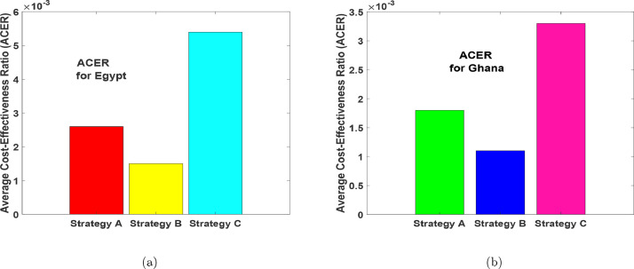
Now, using the formula in (15), we found that Strategy B has the least ACER value, followed by Strategy A, then Strategy C as seen in Fig. 19 (a) and Fig. 19(b) respectively. The result is also clearly shown in Table 3 and Table 6 . Thus, the result of ACER cost analysis support the IAR that, the most effective intervention strategy is Strategy B, followed by Strategy A, and lastly Strategy C.

Fig. 19.

Average cost-effectiveness ratio (ACER) results for Strategies A–C.

Table 3.

Strategies A–C in order of increasing number of COVID-19 infections averted.

Strategy	Total infections averted($\times {10}^5$)	Total cost ($)	ACER	ICER
$\Delta$=No strategy, $(u_1=u_2=0$):	0	0	-	-
C: $u_2\left(t\right)$	1.0348	561.2034	0.0054	0.0054
B: $u_1\left(t\right)$	3.7625	562.5000	0.0015	$4.7535\times {10}^{-6}$
A: $u_1\left(t\right),$$u_2\left(t\right)$	3.8530	996.8271	0.0026	-

Table 6.

Strategies A–C in order of increasing number of COVID-19 infections averted.

Strategy	Total infections averted ($\times {10}^5$)	Total cost ($)	ACER	ICER
$\Delta$=No strategy, $(u_1=u_2=0)$:	0	0	-	-
C: $u_2\left(t\right)$	1.5891	529.6678	0.0033	0.0033
B: $u_1\left(t\right)$	5.1593	562.4772	0.0011	$9.1874\times {10}^{-4}$
A: $u_1\left(t\right),$$u_2\left(t\right)$	5.2420	925.0752	$0.0018$	-

Incremental cost-effectiveness ratio (ICER)

ICER is a cost-effectiveness ratio useful to determine the differences between two alternative control intervention strategies as regards to their costs and benefits. It is calculated using the mathematical expression given as

$$\text{ICER}=\frac{\text{Difference}\text{in}\text{the}\text{costs}\text{for}\text{applying}\text{Strategies}\mathbf{\text{m}}\text{and}\mathbf{\text{n}}}{\text{Difference}\text{in}\text{the}\text{total}\text{number}\text{of}\text{infections}\text{averted}\text{by}\text{implementing}\text{Strategies}\mathbf{\text{m}}\text{and}\mathbf{\text{n}}}.$$ (16)

The corresponding cost to the application of a particular strategy is obtained from the expression given in (8).

6.1. Optimal economic evaluation of the implemented Strategies A–C for Egypt

In view of the simulated optimal control problem for the COVID-19 population dynamics in Egypt as illustrated in Figs. 15(a)–15(f), we compute the cost-effectiveness analysis for Strategies A, B and C.

The ICER values are computed to further affirm the most economical strategy from the other control intervention strategies considered in this study. From the results obtained for the numerical simulations of the optimal control problem, Strategies A–C are ranked according to their increasing order with respect to the total number of COVID-19 infections averted in the community as shown in Table 3.

The ICER is computed for the competing Strategies C and B using the formula in (16) as follows:

$$\begin{array}{cc}\text{ICER(C/}▵)\hfill & ={\displaystyle \frac{561.2034}{1.0348\times {10}^5}}=0.0054,\hfill \\ \text{ICER(B/C)}\hfill & ={\displaystyle \frac{562.5000-561.2034}{3.7625\times {10}^5-1.0348\times {10}^5}}=4.7535\times {10}^{-6}.\hfill \end{array}$$

The computed results (as summarized in Table 3) indicate that the ICER value of strategy C, is higher than that of strategy B. This means that the singular application of contact tracing control $u_2$ is more costly and less effective than when the health protocols-personal protections control $u_1$ only is implemented. Thus, Strategy C is eliminated from the list of alternative control intervention strategies.

Then, it remains to re-compute the ICER for Strategies B and A. The computation is carried out as follows:

$$\begin{array}{cc}\text{ICER(B/}\Delta \text{)}\hfill & ={\displaystyle \frac{562.5000}{3.7625\times {10}^5}}=0.0015,\hfill \\ \text{ICER(A/B)}\hfill & ={\displaystyle \frac{996.8271-562.5000}{3.8530\times {10}^5-3.7625\times {10}^5}}=0.0480.\hfill \end{array}$$

The summary of the calculations is provided in Table 4.

Table 4.

ICER for Strategies A and B.

Strategy	Total infections averted($\times {10}^5$)	Total cost ($)	ACER	ICER
B: $u_1\left(t\right)$	3.7625	562.5000	0.0015	0.0015
A: $u_1\left(t\right),$$u_2\left(t\right)$	3.8530	996.8271	0.0026	0.0480

It is noted from Table 4 that the ICER for Strategy A, is greater than the ICER of Strategy B. Then, this is an implication that the simultaneous implementation of health protocols-personal protections ($u_1$) and contact tracing ($u_2$) control is more costly when compared with the singular application of health protocols-personal protections control $u_1$. Consequently, the application of health protocols-personal protections controls only is the most cost-effective when considering all the three different control interventions applied to the optimal control of COVID-19 in an enclosed population (no natural birth and deaths) in Egypt, under investigation for this particular work. Nevertheless, Figs. 15(a)-15(b) and Table 5 shows that the combination of $u_1$ and $u_2$ (strategy A) has the highest potential of reducing more infections and preventing more susceptible individuals from COVID-19 as time traverses. But, from the ICER analysis, we noticed that such intervention (strategy A) requires a lot of financial resources and human capital.

Table 5.

Projected susceptibility cases prevented for Egypt.

Strategy	100 days	1 year	2 years	3 years
A: $u_1\left(t\right),u_2\left(t\right)$	$8.8424\times {10}^5$	$2.0061\times {10}^6$	$3.3483\times {10}^6$	$4.6904\times {10}^6$
B: $u_1\left(t\right)$	$8.6675\times {10}^5$	$1.9687\times {10}^6$	$3.2862\times {10}^6$	$4.6037\times {10}^6$
C: $u_2\left(t\right)$	$2.0653\times {10}^5$	$5.0455\times {10}^5$	$8.4745\times {10}^5$	$1.1903\times {10}^6$

6.2. Optimal economic evaluation of the implemented Strategies A–C for Ghana

Next, we calculate the ICER values to further affirm the most cost-effective strategy from the other strategies under examination for this particular work as demonstrated in Figs. 16(a)–16(f). Using the simulated results of the optimal control problem, we rank Strategies A–C based on their order of increase as regards the total number of COVID-19 infections averted in the population as presented in Table 6.

For strategies C and B, the ICER is computed based on the formula given in (16) as follows:

$$\begin{array}{cc}\text{ICER(C/}\Delta \text{)}\hfill & ={\displaystyle \frac{529.6678}{1.5881\times {10}^5}}=0.0033,\hfill \\ \text{ICER(B/C)}\hfill & ={\displaystyle \frac{562.4772-529.6678}{5.1593\times {10}^5-1.58818\times {10}^5}}=9.1874\times {10}^{-5}.\hfill \end{array}$$

The results of ICER calculation (as summarized in Table 6) reveal that the ICER value of strategy C, is greater than that of strategy B. By implication, singular implementation of contact tracing control $u_2$ is more costly and less effective compare to when only health protocols-personal protections control $u_1$ is in use. Therefore, Strategy C is discarded from the list of alternative control strategies.

We now face the re-calculation of the ICER for Strategies B and A. The calculations are made as follows:

$$\begin{array}{c}\text{ICER(B/}\Delta \text{)}={\displaystyle \frac{559.8992}{5.1593\times {10}^5}}=0.0011,\hfill \\ \text{ICER(A/B)}={\displaystyle \frac{830.0470-559.8992}{5.24200\times {10}^5-5.1593\times {10}^5}}=0.0327.\hfill \end{array}$$

We provide the summary of the computations in Table 7 .

Table 7.

ICER for Strategies A and B.

Strategy	Total infections averted($\times {10}^5$)	Total cost ($)	ACER	ICER
B: $u_1\left(t\right)$	5.1593	559.8992	0.0011	0.0011
A: $u_1\left(t\right),$$u_2\left(t\right)$	5.2420	830.0470	0.0018	0.0327

It is clearly shown in Table 7 that Strategy A has an ICER value higher that of Strategy B. It follows that the simultaneous use of health protocols-personal protections ($u_1$) and contact tracing ($u_2$) controls is more costly when compared with the singular use of health protocols-personal protections control $u_1$. Conclusively, the use of health protocols-personal protections control only is the most cost-effective when considering all the three different control strategies applied to the dynamics of the COVID-19 population in Ghana under the analysis for this particular study. But, from Figs. 16(a)-16(b) and Table 8 shows that, the implementation of $u_1$ and $u_2$ reduces more infections and protecting more susceptible individuals as time span than using $u_1$. Therefore, the ICER analysis suggests that the optimal intervention (strategy A) will require a lot of financial and human resources in the event of multiple waves of COVID-19 in Ghana.

Table 8.

Projected susceptibility cases prevented for Ghana.

Strategy	100 days	1 year	2 years	3 years
A: $u_1\left(t\right),u_2\left(t\right)$	$1.4367\times {10}^6$	$1.6448\times {10}^6$	$1.6650\times {10}^6$	$1.6851\times {10}^6$
B: $u_1\left(t\right)$	$1.4174\times {10}^6$	$1.6236\times {10}^6$	$1.6435\times {10}^6$	$1.6634\times {10}^6$
C: $u_2\left(t\right)$	$3.9112\times {10}^5$	$4.5704\times {10}^5$	$4.6264\times {10}^5$	$4.6824\times {10}^5$

7. Concluding Remarks

Based on the dynamics of COVID-19 control measures implemented by nations globally. We formulated a new deterministic model to capture the dynamics of the disease in Ghana and Egypt using a ten compartmental model with a standard incidence rate. We hypothetically noticed that the number of undetected recoveries overpasses the number of detected recoveries for the aforementioned countries. Our sensitivity analysis findings suggest that reducing the transmission rates and increasing contact tracing (testing-diagnoses) is possible to hinder the fast spread of COVID-19, and multiple waves of COVID-19 in Ghana and Egypt. Hence, we adjusted our model to include time-variant controls (health protocols-personal protections, contact tracing (testing and diagnoses)). The existence of the optimal control problem and optimal trajectories are established. The outcome of the optimal control analysis shows that the implementation of health protocols-personal protections and contact tracing (testing-diagnoses) reduces more infections as compared to the one control strategy, but costly than the use of only one control strategy.

Disclosure

This is a revised work of the first author’s preprint “A mathematical model and sensitivity assessment of COVID-19 outbreak for Ghana and Egypt” Available at SSRN [48].

Data availability statement

The parameter values (data) used to support the findings of this study have been described in Section 3.

CRediT authorship contribution statement

Joshua Kiddy K. Asamoah: Conceptualization, Methodology, Formal analysis, Writing - original draft, Writing - review & editing. Zhen Jin: Supervision, Funding acquisition, Writing - original draft, Writing - review & editing. Gui-Quan Sun: Supervision, Funding acquisition, Writing - original draft, Writing - review & editing. Baba Seidu: Writing - original draft, Writing - review & editing. Ernest Yankson: Writing - original draft, Writing - review & editing. Afeez Abidemi: Writing - original draft, Writing - review & editing. F.T. Oduro: Writing - original draft, Writing - review & editing. Stephen E. Moore: Writing - original draft, Writing - review & editing. Eric Okyere: Writing - original draft, Writing - review & editing.

Declaration of Competing Interest

The authors declare that they have no known competing financial interests or personal relationships that could have appeared to influence the findings reported in this paper.

Appendix A. The control reproduction number

The evaluation of the control reproduction number ${\mathcal{R}}_c,$ is done using the concept of the next generation matrix approach as iterated in Asamoah et al.[5]. The control reproduction number, ${\mathcal{R}}_c,$ is defined as the number of secondary infections one infected person produces on average throughout its infectious period in the presence of mitigation measures. Thus, we let $G=F{V}^{-1}$ be the next generation matrix which consists of ${\mathcal{F}}_i\left(x\right),$ $v_i^{+}\left(x\right)$ and $v_i^{-}\left(x\right),$ $i=1,2,...,n\in \mathbb{N}$; where $\mathcal{F}\left(x\right)$ is the rate at which a new infection occurs in compartment $i$. Also, $v_i^{+}$ and $v_i^{-}$ are the rate of immigration into compartment $i$ and the rate at which new individuals are transferred from compartment $i$ respectively [5]. Therefore $F$ and $V$ are defined

$$F=\left[\frac{\partial {\mathcal{F}}_i\left(x_0\right)}{\partial x_i}\right]\text{and}V=\left[\frac{\partial {\mathcal{V}}_i\left(x_0\right)}{\partial x_i\left(x_0\right)}\right],$$

where ${\mathcal{V}}_i\left(x\right)=v_i^{-}\left(x\right)-v_i^{+}\left(x\right)$. Now, from Eq. (1), the matrix of $\mathcal{F}\left(x\right)$ and $\mathcal{V}\left(x\right),$ is given as

$$\begin{array}{cc}\hfill {\mathcal{F}}_i\left(x\right)& =\left[\begin{array}{c}{\displaystyle \frac{\beta ({\eta }_{0}E+{\eta }_{1}A+I_s+{\eta }_{2}H)S+(1-{\beta }_1)\beta ({\eta }_{0}E+{\eta }_{1}A+I_s+{\eta }_{2}H)S_P}{N-D-Q}}\\ 0\\ 0\\ 0\end{array}\right],\hfill \\ \hfill {\mathcal{V}}_i\left(x\right)& =\left[\begin{array}{c}(1-f)\rho E+f\gamma E\\ -(1-f)\rho E+\tau A+\sigma A+\varphi A\\ -f\gamma E-\sigma A+(\delta +d)I_s\\ -\delta I_s+rH+\kappa H\end{array}\right].\hfill \end{array}$$

Computation of ${\mathcal{F}}_i\left(x\right)$ and ${\mathcal{V}}_i\left(x\right)$ evaluated at the disease-free equilibrium:

$$(S,E,A,Q,I_s,H,R,R{,}^{A}D{S}_p)=(S^{*},0,0,0,0,0,0,0,0,\frac{\alpha }{\omega }N\left(0\right)),$$

is given as

$$\begin{array}{cc}\hfill F& =\left(\begin{array}{cccc}(\beta {\eta }_0\frac{S^{*}}{N^{*}}+(1-{\beta }_1)\beta {\eta }_0\frac{S_p^{*}}{N^{*}})& (\beta {\eta }_1\frac{S^{*}}{N^{*}}+(1-{\beta }_1)\beta {\eta }_1\frac{S_p^{*}}{N^{*}})& (\beta \frac{S^{*}}{N^{*}}+(1-{\beta }_1)\beta \frac{S_p^{*}}{N^{*}})& (\beta {\eta }_2\frac{S^{*}}{N^{*}}+(1-{\beta }_1)\beta {\eta }_2\frac{S_p^{*}}{N^{*}})\\ 0& 0& 0& 0\\ 0& 0& 0& 0\\ 0& 0& 0& 0\end{array}\right),\hfill \\ \hfill V& =\left(\begin{array}{cccc}\left(\right(1-f)\rho +f\gamma )& 0& 0& 0\\ -(1-f)\rho & (\tau +\sigma +\varphi )& 0& 0\\ -f\gamma & -\sigma & \delta +d& 0\\ 0& 0& -\delta & (r+\kappa )\end{array}\right).\hfill \end{array}$$

Note that, if there are no infectious persons in the population, then $\alpha$ is zero, otherwise, $\alpha$ is a positive constant. Hence, the calculated control (effective) reproduction ${\mathcal{R}}_c$ given in Eqs. (2) and (3) are obtained from

$${\mathcal{R}}_c={\rho }_1\left(F{V}^{-1}\right),$$

where ${\rho }_1$ is the spectral radius of matrix $F{V}^{-1}$.

References

- 1.NSW . 2020. Government: Novel coronavirus 2019 (2019 n-cov) [Google Scholar]; https://www.health.nsw.gov.au/Infectious/factsheets/Pages/novel-coronavirus.
- 2.Smith R.D. Responding to global infectious disease outbreaks: lessons from sars on the role of risk perception, communication and management. Soc Sci Med. 2006;63(12):3113–3123. doi: 10.1016/j.socscimed.2006.08.004. [DOI] [PMC free article] [PubMed] [Google Scholar]
- 3.Rihan F.A., Al-Salti N.S., Anwar M.-N.Y. AIP Conf Proc. Vol. 1982. AIP Publishing LLC; 2018. Dynamics of coronavirus infection in human; p. 020009. [DOI] [Google Scholar]
- 4.worldometer . 2020. Countries in the world by population (2020) [Google Scholar]; https://www.worldometers.info/world-population/population-by-country/.
- 5.Asamoah J.K.K., Owusu M., Jin Z., Oduro F., Abidemi A., Gyasi E.O. Global stability and cost-effectiveness analysis of COVID-19 considering the impact of the environment: using data from Ghana. Chaos Solitons Fractals. 2020:110103. doi: 10.1016/j.chaos.2020.110103. [DOI] [PMC free article] [PubMed] [Google Scholar]
- 6.Organization W.H. 2020. Coronavirus disease (COVID-19) advice for the public. [Google Scholar]; https://www.who.int/emergencies/diseases/novel-coronavirus-2019/advice-for-public.
- 7.BBC . 15 February 2020. Coronavirus: Beijing orders 14-day quarantine for returnees. [Google Scholar]; https://www.bbc.com/news/world-asia-china-51509248.
- 8.Egypttoday . 14 February 2020. Egypt announces first coronavirus infection. [Google Scholar]; https://www.egypttoday.com/Article/1/81641/Egypt-announces-first-Coronavirus-infection.
- 9.Worldometer . 2020. COVID-19 coronavirus pandemic. [Google Scholar]; https://www.worldometers.info/coronavirus/.
- 10.El-Ghitany E. 2020. A short-term forecast scenario for COVID-19 epidemic and allocated hospital readiness in egypt. [Google Scholar]
- 11.Frost I., Osena G., Craig J., Hauck S., Kalanxhi E., Gatalo O., et al. 2020. COVID-19 in middle africa: National projections of total and severe infections under different lockdown scenarios. [DOI] [PMC free article] [PubMed] [Google Scholar]
- 12.Zhao Z., Li X., Liu F., Zhu G., Ma C., Wang L. Prediction of the COVID-19 spread in african countries and implications for prevention and controls: a case study in South Africa, Egypt, Algeria, Nigeria, Senegal and Kenya. Sci Total Environ. 2020:138959. doi: 10.1016/j.scitotenv.2020.138959. [DOI] [PMC free article] [PubMed] [Google Scholar]
- 13.Asamoah J.K.K., Bornaa C., Seidu B., Jin Z. Mathematical analysis of the effects of controls on transmission dynamics of SARS-CoV-2. Alex Eng J. 2020 doi: 10.1016/j.aej.2020.09.033. [DOI] [Google Scholar]
- 14.Sun G.-Q., Wang S.-F., Li M.-T., Li L., Zhang J., Zhang W., et al. Transmission dynamics of covid-19 in Wuhan, China: effects of lockdown and medical resources. Nonlinear Dyn. 2020;101(3):1981–1993. doi: 10.1007/s11071-020-05770-9. [DOI] [PMC free article] [PubMed] [Google Scholar]
- 15.Chowell G., Fenimore P.W., Castillo-Garsow M.A., Castillo-Chavez C. Sars outbreaks in ontario, hong kong and singapore: the role of diagnosis and isolation as a control mechanism. J Theor Biol. 2003;224(1):1–8. doi: 10.1016/S0022-5193(03)00228-5. [DOI] [PMC free article] [PubMed] [Google Scholar]
- 16.A primer on using mathematics to understand covid-19 dynamics: Modeling, analysis and simulations. Infect Dis Model. 2020 doi: 10.1016/j.idm.2020.11.005. [DOI] [PMC free article] [PubMed] [Google Scholar]
- 17.Ngonghala C.N., Iboi E., Eikenberry S., Scotch M., MacIntyre C.R., Bonds M.H., et al. Mathematical assessment of the impact of non-pharmaceutical interventions on curtailing the 2019 novel coronavirus. Math Biosci. 2020:108364. doi: 10.1016/j.mbs.2020.108364. [DOI] [PMC free article] [PubMed] [Google Scholar]
- 18.Hethcote H.W. The mathematics of infectious diseases. SIAM Rev. 2000;42(4):599–653. [Google Scholar]
- 19.Van den Driessche P., Watmough J. Reproduction numbers and sub-threshold endemic equilibria for compartmental models of disease transmission. Math Biosci. 2002;180(1-2):29–48. doi: 10.1016/S0025-5564(02)00108-6. [DOI] [PubMed] [Google Scholar]
- 20.Ivorra B., Ferrández M., Vela-Pérez M., Ramos A. Tech. Rep. Technical report, MOMAT, 03 2020; 2020. Mathematical modeling of the spread of the coronavirus disease 2019 (COVID-19) considering its particular characteristics. the case of China. [DOI] [PMC free article] [PubMed] [Google Scholar]
- 21.Cintrón-Arias A., Castillo-Chávez C., Bettencourt L., Lloyd A.L., Banks H.T. The estimation of the effective reproductive number from disease outbreak data. 2020 doi: 10.3934/mbe.2009.6.261. arXiv: 2004.06827. [DOI] [PubMed] [Google Scholar]
- 22.Chowell G., Hyman J.M., Bettencourt L.M., Castillo-Chavez C. Springer; 2009. Mathematical and statistical estimation approaches in epidemiology. [Google Scholar]
- 23.Martcheva M. Vol. 61. Springer; 2015. An introduction to mathematical epidemiology. [Google Scholar]
- 24.JHU . 2020. Coronavirus Resource Center: Center for Systems Science and Engineering (CSSE) at Johns Hopkins University (JHU) [Google Scholar]; https://coronavirus.jhu.edu/map.html.
- 25.Wang H., Wang Z., Dong Y., Chang R., Xu C., Yu X., et al. Phase-adjusted estimation of the number of coronavirus disease 2019 cases in Wuhan, China. Cell Discov. 2020;6(1):1–8. doi: 10.1038/s41421-020-0148-0. [DOI] [PMC free article] [PubMed] [Google Scholar]
- 26.Lin Q., Zhao S., Gao D., Lou Y., Yang S., Musa S.S., et al. A conceptual model for the coronavirus disease 2019 (COVID-19) outbreak in Wuhan, China with individual reaction and governmental action. Int J Infect Dis. 2020;93:211–216. doi: 10.1016/j.ijid.2020.02.058. [DOI] [PMC free article] [PubMed] [Google Scholar]
- 27.Rong X., Yang L., Chu H., Fan M. Effect of delay in diagnosis on transmission of COVID-19. Math Biosci Eng. 2020;17(3):2725–2740. doi: 10.3934/mbe.2020149. [DOI] [PubMed] [Google Scholar]
- 28.McGee J. 2020. COVID-19 Modeling. [Google Scholar]; https://www.mathworks.com/matlabcentral/fileexchange/74632-covid-19-modeling.
- 29.Asamoah J.K.K., Jin Z., Sun G.-Q., Li M.Y. A Deterministic Model for Q Fever Transmission Dynamics within Dairy Cattle Herds: Using Sensitivity Analysis and Optimal Controls. Comput Math Methods Med. 2020;2020 doi: 10.1155/2020/6820608. [DOI] [PMC free article] [PubMed] [Google Scholar]
- 30.Mpeshe S.C., Haario H., Tchuenche J.M. A mathematical model of rift valley fever with human host. Acta Biotheor. 2011;59(3-4):231–250. doi: 10.1007/s10441-011-9132-2. [DOI] [PubMed] [Google Scholar]
- 31.Asamoah J.K.K., Jin Z., Sun G.-Q. Non-seasonal and seasonal relapse model for Q fever disease with comprehensive cost-effectiveness analysis. Results Phys. 2021:103889. doi: 10.1016/j.rinp.2021.103889. [DOI] [PMC free article] [PubMed] [Google Scholar]
- 32.Ullah S., Khan M.A. Modeling the impact of non-pharmaceutical interventions on the dynamics of novel coronavirus with optimal control analysis with a case study. Chaos Solitons Fractals. 2020;139:110075. doi: 10.1016/j.chaos.2020.110075. [DOI] [PMC free article] [PubMed] [Google Scholar]
- 33.Asamoah J.K.K., Oduro F.T., Bonyah E., Seidu B. Modelling of rabies transmission dynamics using optimal control analysis. J Appl Math. 2017;2017 doi: 10.1155/2017/2451237. [DOI] [Google Scholar]
- 34.Fleming W.H., Rishel R.W. Vol. 1. Springer Science & Business Media; 2012. Deterministic and stochastic optimal control. [Google Scholar]
- 35.Joshi H.R. Optimal control of an hiv immunology model. Optimal control applications and methods. 2002;23(4):199–213. doi: 10.1002/oca.710. [DOI] [Google Scholar]
- 36.Asamoah J.K.K., Nyabadza F., Jin Z., Bonyah E., Khan M.A., Li M.Y., et al. Backward bifurcation and sensitivity analysis for bacterial meningitis transmission dynamics with a nonlinear recovery rate. Chaos Solitons Fractals. 2020;140:110237. doi: 10.1016/j.chaos.2020.110237. [DOI] [Google Scholar]
- 37.Okosun K.O., Rachid O., Marcus N. Optimal control strategies and cost-effectiveness analysis of a malaria model. Biosyst. 2013;111(2):83–101. doi: 10.1016/j.biosystems.2012.09.008. [DOI] [PubMed] [Google Scholar]
- 38.Agusto F., Adekunle A. Optimal control of a two-strain tuberculosis-hiv/aids co-infection model. Biosyst. 2014;119:20–44. doi: 10.1016/j.biosystems.2014.03.006. [DOI] [PubMed] [Google Scholar]
- 39.Asamoah J.K.K., Nyabadza F., Seidu B., Chand M., Dutta H. Mathematical modelling of bacterial meningitis transmission dynamics with control measures. Comput Math Methods Med. 2018;2018 doi: 10.1155/2018/2657461. [DOI] [PMC free article] [PubMed] [Google Scholar]
- 40.Alzahrani E.O., Ahmad W., Khan M.A., Malebary S.J. Optimal control strategies of zika virus model with mutant. Commun Nonlinear Sci Numer Simul. 2021;93:105532. doi: 10.1016/j.cnsns.2020.105532. [DOI] [Google Scholar]
- 41.Lenhart S., Workman J.T. Chapman and Hall/CRC; 2007. Optimal control applied to biological models. [Google Scholar]
- 42.Olaniyi S., Obabiyi O., Okosun K., Oladipo A., Adewale S. Mathematical modelling and optimal cost-effective control of covid-19 transmission dynamics. Eur Phys J Plus. 2020;135(11):1–20. doi: 10.1140/epjp/s13360-020-00954-z. [DOI] [PMC free article] [PubMed] [Google Scholar]
- 43.Olaniyi S., Okosun K., Adesanya S., Lebelo R. Modelling malaria dynamics with partial immunity and protected travellers: optimal control and cost-effectiveness analysis. J Biol Dyn. 2020;14(1):90–115. doi: 10.1080/17513758.2020.1722265. [DOI] [PubMed] [Google Scholar]
- 44.Agusto F., Leite M. Optimal control and cost-effective analysis of the 2017 meningitis outbreak in Nigeria. Infect Dis Model. 2019;4:161–187. doi: 10.1016/j.idm.2019.05.003. [DOI] [PMC free article] [PubMed] [Google Scholar]
- 45.Agusto F.B., ELmojtaba I.M. Optimal control and cost-effective analysis of malaria/visceral leishmaniasis co-infection. PLoS One. 2017;12(2):e0171102. doi: 10.1371/journal.pone.0171102. [DOI] [PMC free article] [PubMed] [Google Scholar]
- 46.Okyere E., Olaniyi S., Bonyah E. Analysis of zika virus dynamics with sexual transmission route using multiple optimal controls. Scientific African. 2020;9:e00532. [Google Scholar]
- 47.Oke S.I., Matadi M.B., Xulu S.S. Cost-effectiveness analysis of optimal control strategies for breast cancer treatment with ketogenic diet. Far East J Math Sci. 2018;109(2):303–342. [Google Scholar]
- 48.Asamoah J., Jin Z., Seidu B., Sun G., Alzahrani F., Oduro F.. A mathematical model and sensitivity assessment of covid-19 outbreak for ghana and egypt. Available at SSRN.
Associated Data
This section collects any data citations, data availability statements, or supplementary materials included in this article.