A fractional-order model describing the dynamics of the novel coronavirus (COVID-19) with nonsingular kernel

Abstract

In this paper, we investigate an epidemic model of the novel coronavirus disease or COVID-19 using the Caputo–Fabrizio derivative. We discuss the existence and uniqueness of solution for the model under consideration, by using the the Picard–Lindelöf theorem. Further, using an efficient numerical approach we present an iterative scheme for the solutions of proposed fractional model. Finally, many numerical simulations are presented for various values of the fractional order to demonstrate the impact of some effective and commonly used interventions to mitigate this novel infection. From the simulation results we conclude that the fractional order epidemic model provides more insights about the disease dynamics.

1. Introduction

The novel Coronavirus COVID-19 is an infectious respiratory diseases, emerged in November 2019 in Hubei Wuhan city of China. After the outbreak of COVID-19 was noticed, the world health organization (WHO) announce the COVID-19 a pandemic diseases on March 2020. Since then this infection reach the whole word due to its fast transmission. The COVID-19 symptoms reported so far are not specific, witch does not allow the detection of infected cases quickly. In fact the infection of this new virus has symptoms similar to those of influenza which includes fever, respiratory signs such as cough, muscle pain and fatigue. the incubation period of this novel infection ranges from 1 to 14 days [1]. In more sever cases the infection leads to severe pneumonia respiratory syndrome even death, It has noticed that the most severe cases seem to concern vulnerable individuals (the elderly, people suffering of chronic diseases). Other characteristics of the COVID-19 pandemic is that there is no specific treatment and no effective vaccine, certain treatments are being tested in clinical trial. The COVID-19 can be spread from person to person through close contact with an infected person. In the absence of effective treatment the physical distancing strategy is adopted to minimize the spread of infection. Other characteristics of COVID-19 is that a person may be asymptomatic and can be contagious at same time and the strategy adopted in this situation is the quarantine strategy. Although a large part of mystery has been seen in the evolution of the COVID-19 and remains difficult to provide [2]. As part of contribution against the COVID-19 mathematical model seem appropriate to understand the spread of the virus and allows as figure out the effect of the strategy intervention adopted to slow down the spread of the virus, perhaps one major goal is to flatten the curve of the epidemic.

Different approaches have been adopted to control the outbreaks of the novel COVID-19 pandemic. Mathematical modeling is considered as one of useful tool to explore the transmission dynamics of a disease and help the policy-makers to set some effective strategy to control the disease outbreak. These mathematical model generally given in terms of differential equations allows us to test a wide of possible scenarios of the dynamic of the virus in a short period of time. It is possible that some suspicious parameters associated with certain model limit the accuracy of predictions in the beginning of an epidemic. However, even in the absence of available data, the knowledge acquired during previous known epidemics makes it possible to build an initial model to evaluate the intervention of the strategy to be adopted. Most of the recent model of COVID-19 are derived from the SIR model, witch describes the transitions between population of susceptible ($S$), infectious ($I$) and recovery ($R$) individuals. Duccio and Francesco proposed a deterministic model to analyze the dynamical patterns and future prediction of the outbreaks in three epicenters of novel COVID-19 [3]. Asamoah et al., [4] formulated a mathematical model with the environmental viral load and suggested some effective intervention strategies using optimal control approach. Ullah and Khan suggested a novel mathematical model to explore the role of some useful public interventions on the dynamics of COVID-19 in Pakistani population [5]. Tang et al., [6] developed a realistic mathematical model to study the dynamics and influence of enhancement of different public health interventions against COVID-19 outbreak in China.

Epidemic models based on fractional derivatives is another effective approach to study the dynamics of an infectious disease in a better way. Mathematical models with fractional order differential equation provides more insights about a phenomena because they posses the memory effect and are nonlocal in nature. The use of mathematical models in terms of fractional differential equations gain much interest in last few years. The goal is to overcome some limitation related to the model depends on classical derivatives. Mathematical models with fractional derivative are suitable to demonstrate some natural phenomena including an infectious diseases under consideration [7], [8], [9], [10]. Different non-integer order operators with singular and nonsingular kernel were suggested in literature [11], [12], [13]. The application of these fractional operators can be found in Baleanu et al. [14], Ullah et al. [15], 16] and references therein. A number of mathematical models base on different fractional order operators were proposed in recent few months to analyze the complex transmission patterns of novel COVID-19. A fractional order model using Caputo–Fabrizio operator is studied in Baleanu et al. [17] to analyzed the effect of memory index and various parameters on the dynamics COVID-19. A novel fractional-fractal operator is used to formulate a mathematical model to explore the impact of lockdown on the dynamics of COVID-19 in Atangana [18]. A fractional order model based on Atangana–Baleanu operator was formulated in Khan and Atangana [19] to predict the COVID-19 situation in Wuhan, China.

In the study in hand, we extend a COVID-19 virus transmission model suggested in Tang et al. [6] under Caputo–Fabrizio fractional derivative. Initially, we discuss the model formulation using classical integer-order differential equation and the reformulated the fractional order COVID-19 model and then prove the existence and untidiness of the model solution. Moreover, the COVID-19 model with Caputo–Fabrizio operator is solved numerically, and the graphical impact of various parameters is depicted for different values of fractional order. The rest of paper is organized as: The next section consists the basic definition regarding fractional calculus. The model formulation using Caputo–Fabrizio derivative is presented in Section 3. The exitance and uniqueness of the model solution is provided in Section 4. The iterative scheme along with simulations and discussion is presented in Section 6. Finally, a brief conclusion of the present work is given in Section 5.

2. Preliminaries

In this section we present essential definitions and result from fractional calculus. The aim is to recall the definitions and proprieties of the Caputo–Fabrizio derivatives used in this paper. the author can see [13] for more detail.

Let $H^1\left(\right]a,b\left[\right)=\{f\mid f\in L^2\left(\right]a,b\left[\right),\text{and}{f}^{\prime }\in L^2\left(\right]a,b\left[\right)\},$ where the $L^2\left(\right]a,b\left[\right)$ is the usual Exergue space of square integrable function on the interval $]a,b[$.

Definition 2.1 Caputo and Fabrizio [13] —

Let $f\in H^1\left(\right]a,b\left[\right)$ and $\nu \in ]0,1[,$ then the Caputo–Fabrizio fractional derivative is defined to be

$${}^{CF}{D}_t^{\nu }\left(f\left(t\right)\right)=\frac{M\left(\nu \right)}{1-\nu }{\int }_a^t{f}^{\prime }\left(s\right)\exp (-\nu \frac{t-s}{1-\nu })ds,$$ (1)

where, $M\left(\nu \right)$ define a normalization function with $M\left(0\right)=M\left(1\right)=1$.

Remark 1 Caputo and Fabrizio [13] —

• 1.According to (1) when $f\left(t\right)$ is constant then ${}^{CF}{D}_t^{\nu }\left(f\left(t\right)\right)=0$.
• 2.If $f\notin H^1\left(\right]a,b\left[\right)$ then the Caputo–Fabrizio fractional derivative is defined also for
  $f\in L^1\left(\right]-\infty ,b\left[\right)$ having order $\nu \in ]0,1[$ as

  $${}^{CF}{D}_t^{\nu }\left(f\left(t\right)\right)=\frac{\nu M\left(\nu \right)}{1-\nu }{\int }_{-\infty }^t(f\left(t\right)-f\left(s\right))\exp (-\nu \frac{t-s}{1-\nu })ds.$$ (2)
• 3.
  If we put $\rho =\frac{1-\nu }{\nu }\in ]0,+\infty [,$ then $\nu =\frac{1}{\rho +1}\in ]0,1[$. The Eq. (1) become

  $${}^{CF}{D}_t^{\nu }\left(f\left(t\right)\right)=\frac{N\left(\rho \right)}{\rho }{\int }_a^t{f}^{\prime }\left(s\right)\exp (-\frac{t-s}{\rho })ds.$$ (3)

  where $\rho \in ]0,+\infty [$ and $N\left(\rho \right)$ is the relative normalization term of $M\left(\nu \right),$ such that $N\left(0\right)=N(+\infty )=1$.

Remark 2

Because of the singularity when $\nu =1$ in (1) the case $\nu =1$ is shown to be as the limit ${\displaystyle \underset{\nu \to 1}{\lim }{}^{CF}{D}_t^{\nu }\left(f\left(t\right)\right),}$ knowing in addition that ${\displaystyle \underset{\rho \to 0}{\lim }\frac{1}{\rho }\exp (-\frac{t-s}{\rho })=\delta (t-s)}$ we have

$$\begin{array}{cc}\hfill \underset{\nu \to 1}{\lim }{}^{CF}{D}_t^{\nu }\left(f\left(t\right)\right)& =f^{\prime }\left(t\right).\hfill \\ \hfill \underset{\nu \to 0}{\lim }{}^{CF}{D}_t^{\nu }\left(f\left(t\right)\right)& =f\left(t\right)-f\left(a\right).\hfill \end{array}$$

2.1. The associated fractional integral

The corresponding integral of order $0<\nu <1$ is a natural requirement after defining the fractional derivative of order $0<\nu <1$. The above Caputo–Fabrizio operator described in (1) was modified by Losanda and Nieto [20] and we have the following definition.

Definition 2.2 Losada and Nieto [20] —

Let $f\in H^1\left(\right]a,b\left[\right)$ and $\nu \in ]0,1[,$ then the Caputo–Fabrizio fractional derivative is defined to be

$${}^{CF}{D}_t^{\nu }\left(f\left(t\right)\right)=\frac{(2-\nu )M\left(\nu \right)}{2(1-\nu )}{\int }_a^t{f}^{\prime }\left(s\right)\exp (-\nu \frac{t-s}{1-\nu })ds.$$ (4)

The fractional integral corresponding to (4) is then defined as follows.

Definition 2.3 Losada and Nieto [20] —

Let $0<\nu <1,$ then the integral of non integer order $\nu$ of a function $f$ is given as follows:

$${}^{CF}{I}^{\nu }\left(f\left(t\right)\right)=\frac{(2-2\nu )}{(2-\nu )M\left(\nu \right)}f\left(t\right)+\frac{2\nu }{(2-\nu )M\left(\nu \right)}{\int }_0^{t}f\left(s\right)ds,t\ge 0.$$ (5)

We have this useful proposition with constant use in the rest of the paper.

Proposition 2.1 Losada and Nieto [20] —

For a differential equation having fractional order$0<\nu <1$

$${}^{CF}{D}_t^{\nu }\left(f\left(t\right)\right)=h\left(t\right),T\ge 0.$$ (6)

Then we have

$$f\left(t\right)-f\left(0\right)={}^{CF}{I}^{\nu }\left(h\left(t\right)\right)=\frac{(2-2\nu )}{M\left(\nu \right)(2-\nu )}h\left(t\right)+\frac{2\nu }{(2-\nu )M\left(\nu \right)}{\int }_0^{t}h\left(s\right)ds,t\ge 0.$$ (7)

3. Mathematical model

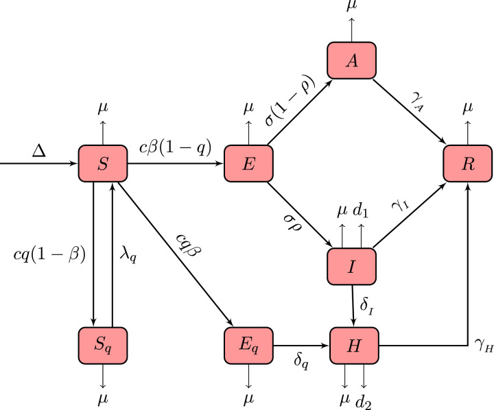
In this section, we consider the deterministic COVID-19 model proposed in Tang et al. [6]. Initially, we reformulate the model by adding the birth rate $\Delta$ and the natural death rate $\mu$. Further, the classical integer order model is then extended to fractional order using Caputo–Fabrizio derivative with nonsingular exponential type kernel. The biological meaning of the model parameters is described in Table 1 and the transition between various population classes is shown in Fig. 1 . The formulated mathematical model for the transmission of a novel COVID-19 pandemic is given by the following system of equations:

$$\begin{array}{ccc}\hfill \frac{dS}{dt}& =& \Delta -(\beta c+cq(1-\beta ))S(I+\theta A)+{\lambda }_q{S}_q-\mu S,\hfill \\ \hfill \frac{dE}{dt}& =& \beta c(1-q)S(I+\theta A)-(\sigma +\mu )E,\hfill \\ \hfill \frac{dI}{dt}& =& \sigma \rho E-({\delta }_{{}_I}+{\gamma }_{{}_I}+\mu +d_1)I,\hfill \\ \hfill \frac{dA}{dt}& =& \sigma (1-\rho )E-(\mu +{\gamma }_{{}_A})A,\hfill \\ \hfill \frac{d{S}_q}{dt}& =& (1-\beta )cqS(I+\theta A)-({\lambda }_q+\mu )S_q,\hfill \\ \hfill \frac{d{E}_q}{dt}& =& \beta cqS(I+\theta A)-(\mu +{\delta }_q)E_q,\hfill \\ \hfill \frac{dH}{dt}& =& {\delta }_{{}_I}I+{\delta }_q{E}_q-({\gamma }_{{}_H}+\mu +d_2)H,\hfill \\ \hfill \frac{dR}{dt}& =& {\gamma }_{{}_A}A+{\gamma }_{{}_I}I+{\gamma }_{{}_H}H-\mu R.\hfill \end{array}$$ (8)

In the model described in (8), the total human population denoted by $N$ at time $t$ is divided into eight different classes: susceptible $S,$ exposed $E,$ symptomatic (infectious with clinical symptoms) $I,$ asymptomatic (infectious but not yet show any clinical symptoms) $A,$ quarantined susceptible individuals $S_q,$ quarantined/isolated exposed individuals $E_q,$ hospitalized individuals $H,$ and finally the recovered or removed individuals $R$. Mathematical models with integer order derivatives play an important role and have their significant to understand the dynamic of epidemiological system. However, it is known that a model based on classical derivatives have some limitations. Theses systems do not posses memory or non local effects and therefore, the models with integer order derivatives are some time not suitable. To deal with this limitation many model of epidemiology are converted to fractional differential equations. In fractional differential calculus the differential operators used are non integer and possesses memory impacts and are efficient to explore many natural phenomena, and facts having non local dynamics behavior. In the next subsection of the paper, we are reconstructed the classical model (8) by applying the Caputo–Fabrizio fractional derivative of order $\nu \in (0,1]$.

Table 1.

Description of the parameters of the system (9).

Parameter	Description	Estimated value	Source
$\Delta$	Birth rate	294	Estimated [21]
$\mu$	Natural death rate	1/76.79	[21]
$c$	Contact rate	14.78	[6]
$\beta$	Probability of transmission per contact	$2.1011\times {10}^{-8}$	[6]
$q$	Quarantined rate of exposed living to $E_q$ compartment	$1.88\times {10}^{-7}$	[6]
$\sigma$	Transition rate from the $E$ to $I$ compartments	1/7	[6]
${\lambda }_q$	The rate of isolation release	1/14	[6]
$\rho$	Probability for having symptoms among infected person	0.8683	[6]
${\delta }_{{}_I}$	Transition rate from $I$ to $H$	0.1326	[6]
${\delta }_q$	Transition rate from $E_q$ to $H$	0.1259	[6]
${\gamma }_{{}_A}$	Recovery rate of pre symptomatic person	0.1397	[6]
${\gamma }_{{}_I}$	Recovery rate of infected person	0.33029	[6]
${\gamma }_{{}_H}$	Recovery rate of quarantined person	0.11624	[6]
$d_1$	Infected death rate	$1.7826\times {10}^{-5}$	[6]
$d_2$	Quarantined death rate	$1.7826\times {10}^{-5}$	[6]
$\theta$	Infectiousness rate due to $A$ class	0.02	[19]

Fig. 1.

Diagram of different stages of transmission of a novel coronavirus in different compartment.

3.1. The Caputo–Fabrizio COVID-19 model

In this section we introduce the fractional COVID-19 epidemic by utilizing the Caputo–Fabrizio operator. For this model we suppose that in each compartment have a natural death at rate $\mu$. To formulate the fractional model we replace the classical derivative in (8) by the Caputo–Fabrizio fractional derivative having order $0<\nu <1$. Thus, we obtain the following system

$$\begin{array}{ccc}\hfill {}^{CF}{D}_t^{\nu }\left(S\left(t\right)\right)& =& \Delta -(\beta c+cq(1-\beta ))S(I+\theta A)+{\lambda }_q{S}_q-\mu S,\hfill \\ \hfill {}^{CF}{D}_t^{\nu }\left(E\left(t\right)\right)& =& \beta c(1-q)S(I+\theta A)-(\sigma +\mu )E,\hfill \\ \hfill {}^{CF}{D}_t^{\nu }\left(I\left(t\right)\right)& =& \sigma \rho E-({\delta }_{{}_I}+{\gamma }_{{}_I}+\mu +d_1)I,\hfill \\ \hfill {}^{CF}{D}_t^{\nu }\left(A\left(t\right)\right)& =& \sigma (1-\rho )E-(\mu +{\gamma }_{{}_A})A,\hfill \\ \hfill {}^{CF}{D}_t^{\nu }\left(S_q\left(t\right)\right)& =& (1-\beta )cqS(I+\theta A)-({\lambda }_q+\mu )S_q,\hfill \\ \hfill {}^{CF}{D}_t^{\nu }\left(E_q\left(t\right)\right)& =& \beta cqS(I+\theta A)-(\mu +{\delta }_q)E_q,\hfill \\ \hfill {}^{CF}{D}_t^{\nu }\left(H\left(t\right)\right)& =& {\delta }_{{}_I}I+{\delta }_q{E}_q-({\gamma }_{{}_H}+\mu +d_2)H,\hfill \\ \hfill {}^{CF}{D}_t^{\nu }\left(R\left(t\right)\right)& =& {\gamma }_{{}_A}A+{\gamma }_{{}_I}I+{\gamma }_{{}_H}H-\mu R.\hfill \end{array}$$ (9)

In addition with the following initial values:

$$\begin{array}{ccc}\hfill S\left(0\right)& =& S_0\le 0,E\left(0\right)=E_0\le 0,I\left(0\right)=I_0\le 0,A\left(0\right)=A_0\le 0,S_q\left(0\right)=S_{q0}\le 0,\hfill \\ \hfill E_q\left(0\right)& =& E_{q0}\le 0H\left(0\right)=H_0\le 0,R\left(0\right)=R_0\le 0.\hfill \end{array}$$ (10)

All parameter used the system (9) are considered to be positive constant, and their biological description are presented in the following table.

The total dynamic of the fractional model of COVID-19 described in (9) is given by the following equation

$$\begin{array}{ccc}\hfill N^{\prime }\left(t\right)& =& \Delta -\mu N-(d_{1}I+d_{2}H)\hfill \\ & \le & \Delta -\mu N.\hfill \end{array}$$ (11)

When $t$ goes to $\infty ,$ we get $N\le \frac{\Delta }{\mu }$.

Proposition 3.1

The biological feasible region for the Caputo–Fabrizio fractional system(9)is

$$\Omega =\{(S,E,I,A,S_q,E_q,H,R)\in {\mathbb{R}}_{+}^8:0\le S+E+I+A+S_q+E_q+H+R\le \frac{\Delta }{\mu }\}.$$ (12)

4. Existence and uniqueness of solution of system (9)

We investigate the existence and uniqueness of the solution of the system (9) with initial condition (10), using fixed point theory and Picard–Lindelöf technique. To proceeds further we Utilize the fractional integral operator in Caputo–Fabrizio sense defined by (5) to both sides of equations in system (9) and using Proposition 2.1, we get

$$\begin{array}{ccc}\hfill S\left(t\right)-S\left(0\right)& =& {}^{CF}{I}^{\nu }(\Delta -(\beta c+cq(1-\beta ))S(I+\theta A)+{\lambda }_q{S}_q-\mu S),\hfill \\ \hfill E\left(t\right)-E\left(0\right)& =& {}^{CF}{I}^{\nu }(\beta c(1-q)S(I+\theta A)-(\sigma +\mu )E),\hfill \\ \hfill I\left(t\right)-I\left(0\right)& =& {}^{CF}{I}^{\nu }(\sigma \rho E-({\delta }_{{}_I}+{\gamma }_{{}_I}+\mu +d_1)I),\hfill \\ \hfill A\left(t\right)-A\left(0\right)& =& {}^{CF}{I}^{\nu }(\sigma (1-\rho )E-(\mu +{\gamma }_{{}_A})A),\hfill \\ \hfill S_q\left(t\right)-S_q\left(0\right)& =& {}^{CF}{I}^{\nu }((1-\beta )cqS(I+\theta A)-({\lambda }_q+\mu )S_q),\hfill \\ \hfill E_q\left(t\right)-E_q\left(0\right)& =& {}^{CF}{I}^{\nu }(\beta cqS(I+\theta A)-(\mu +{\delta }_q)E_q,\hfill \\ \hfill H\left(t\right)-H\left(0\right)& =& {}^{CF}{I}^{\nu }({\delta }_{{}_I}I+{\delta }_q{E}_q-({\gamma }_{{}_H}+\mu +d_2)H),\hfill \\ \hfill R\left(t\right)-R\left(0\right)& =& {}^{CF}{I}^{\nu }({\gamma }_{{}_A}A+{\gamma }_{{}_I}I+{\gamma }_{{}_H}H-\mu R).\hfill \end{array}$$ (13)

System (13) reads in terms of kernels

$$\begin{array}{ccc}\hfill S\left(t\right)-S\left(0\right)& =& \frac{2(1-\nu )}{\mathtt{M}\left(\nu \right)(2-\nu )}{K}_1(S,t)+\frac{2\nu }{\mathtt{M}\left(\nu \right)(2-\nu )}{\int }_0^t{K}_1(S,r)dr,\hfill \\ \hfill E\left(t\right)-E\left(0\right)& =& \frac{2(1-\nu )}{\mathtt{M}\left(\nu \right)(2-\nu )}{K}_2(E,t)+\frac{2\nu }{\mathtt{M}\left(\nu \right)(2-\nu )}{\int }_0^t{K}_2(E,r)dr,\hfill \\ \hfill I\left(t\right)-I\left(0\right)& =& \frac{2(1-\nu )}{\mathtt{M}\left(\nu \right)(2-\nu )}{K}_3(I,t)+\frac{2\nu }{\mathtt{M}\left(\nu \right)(2-\nu )}{\int }_0^t{K}_3(I,r)dr,\hfill \\ \hfill A\left(t\right)-A\left(0\right)& =& \frac{2(1-\nu )}{\mathtt{M}\left(\nu \right)(2-\nu )}{K}_4(A,t)+\frac{2\nu }{\mathtt{M}\left(\nu \right)(2-\nu )}{\int }_0^t{K}_3(A,r)dr,\hfill \\ \hfill S_q\left(t\right)-S_q\left(0\right)& =& \frac{2(1-\nu )}{\mathtt{M}\left(\nu \right)(2-\nu )}{K}_5(S_q,t)+\frac{2\nu }{\mathtt{M}\left(\nu \right)(2-\nu )}{\int }_0^t{K}_5(S_q,r)dr,\hfill \\ \hfill E_q\left(t\right)-E_q\left(0\right)& =& \frac{2(1-\nu )}{\mathtt{M}\left(\nu \right)(2-\nu )}{K}_6(E_q,t)+\frac{2\nu }{\mathtt{M}\left(\nu \right)(2-\nu )}{\int }_0^t{K}_6(E_q,r)dr,\hfill \\ \hfill H\left(t\right)-H\left(0\right)& =& \frac{2(1-\nu )}{\mathtt{M}\left(\nu \right)(2-\nu )}{K}_7(H,t)+\frac{2\nu }{\mathtt{M}\left(\nu \right)(2-\nu )}{\int }_0^t{K}_7(H,r)dr,\hfill \\ \hfill R\left(t\right)-R\left(0\right)& =& \frac{2(1-\nu )}{\mathtt{M}\left(\nu \right)(2-\nu )}{K}_8(R,t)+\frac{2\nu }{\mathtt{M}\left(\nu \right)(2-\nu )}{\int }_0^t{K}_8(R,r)dr,\hfill \end{array}$$ (14)

where the kernels are given by

$$\begin{array}{ccc}\hfill K_1(S,t)& =& \Delta -(\beta c+cq(1-\beta ))S\left(t\right)(I\left(t\right)+A\left(t\right))+{\lambda }_q{S}_q\left(t\right)-\mu S\left(t\right),\hfill \\ \hfill K_2(E,t)& =& \beta c(1-q)S\left(t\right)\left(I\right(t)+A(t\left)\right)-(\sigma +\mu )E\left(t\right),\hfill \\ \hfill K_3(I,t)& =& \sigma \rho E\left(t\right)-({\delta }_{{}_I}+{\gamma }_{{}_I}+\mu +d_1)I\left(t\right),\hfill \\ \hfill K_4(A,t)& =& \sigma (1-\rho )E\left(t\right)-(\mu +{\gamma }_{{}_A})A\left(t\right),\hfill \\ \hfill K_5(S_q,t)& =& (1-\beta )cqS\left(t\right)(I\left(t\right)+A\left(t\right))-({\lambda }_q+\mu )S_q\left(t\right),\hfill \\ \hfill K_6(E_q,t)& =& \beta cqS\left(t\right)(I\left(t\right)+A\left(t\right))-(\mu +{\delta }_q)E_q\left(t\right),\hfill \\ \hfill K_7(H,t)& =& {\delta }_{{}_I}I\left(t\right)+{\delta }_q{E}_q\left(t\right)-({\gamma }_{{}_H}+\mu +d_2)H\left(t\right),\hfill \\ \hfill K_8(R,t)& =& {\gamma }_{{}_A}A\left(t\right)+{\gamma }_{{}_I}I\left(t\right)+{\gamma }_{{}_H}H\left(t\right)-\mu R\left(t\right).\hfill \end{array}$$ (15)

Further, utilizing the Picard iterations are given by

$$\begin{array}{ccc}\hfill S_{n+1}\left(t\right)& =& \frac{2(1-\nu )}{M\left(\nu \right)(2-\nu )}{K}_1(S_n,t)+\frac{2\nu }{M\left(\nu \right)(2-\nu )}{\int }_0^t{K}_1(S_n,r)\mathit{dr},\hfill \\ \hfill E_{n+1}\left(t\right)& =& \frac{2(1-\nu )}{M\left(\nu \right)(2-\nu )}{K}_2(E_n,t)+\frac{2\nu }{M\left(\nu \right)(2-\nu )}{\int }_0^t{K}_2(E_n,r)\mathit{dr},\hfill \\ \hfill I_{n+1}\left(t\right)& =& \frac{2(1-\nu )}{M\left(\nu \right)(2-\nu )}{K}_3(I_n,t)+\frac{2\nu }{M\left(\nu \right)(2-\nu )}{\int }_0^t{K}_3(I_n,r)\mathit{dr},\hfill \\ \hfill A_{n+1}\left(t\right)& =& \frac{2(1-\nu )}{M\left(\nu \right)(2-\nu )}{K}_4(A_n,t)+\frac{2\nu }{M\left(\nu \right)(2-\nu )}{\int }_0^t{K}_4(A_n,r)\mathit{dr},\hfill \\ \hfill {S_q}_{n+1}\left(t\right)& =& \frac{2(1-\nu )}{M\left(\nu \right)(2-\nu )}{K}_5({S_q}_n,t)+\frac{2\nu }{M\left(\nu \right)(2-\nu )}{\int }_0^t{K}_5({S_q}_n,r)\mathit{dr},\hfill \\ \hfill {E_q}_{n+1}\left(t\right)& =& \frac{2(1-\nu )}{M\left(\nu \right)(2-\nu )}{K}_6({S_q}_n,t)+\frac{2\nu }{M\left(\nu \right)(2-\nu )}{\int }_0^t{K}_6({E_q}_n,r)\mathit{dr},\hfill \\ \hfill H_{n+1}\left(t\right)& =& \frac{2(1-\nu )}{M\left(\nu \right)(2-\nu )}{K}_7(H_n,t)+\frac{2\nu }{M\left(\nu \right)(2-\nu )}{\int }_0^t{K}_7(H_n,r)\mathit{dr},\hfill \\ \hfill R_{n+1}\left(t\right)& =& \frac{2(1-\nu )}{M\left(\nu \right)(2-\nu )}{K}_8(R_n,t)+\frac{2\nu }{M\left(\nu \right)(2-\nu )}{\int }_0^t{K}_8(R_n,r)\mathit{dr}.\hfill \end{array}$$ (16)

Next, we rewrite the system (9) in the following form

$$\{\begin{array}{cc}{}^{CF}{D}_t^{\nu }Y\left(t\right)\hfill & =F(t,Y(t\left)\right),\hfill \\ Y\left(0\right)=Y_0\hfill & 0<t<T,\hfill \end{array}$$ (17)

Where, the vector variable $Y\left(t\right)={(S\left(t\right),E\left(t\right),I\left(t\right),A\left(t\right),S_q\left(t\right),E_q\left(t\right),H\left(t\right),R\left(t\right))}^t$ and vector function $F(t,Y(t\left)\right)$ is defined by

$$F(t,Y\left(t\right))=\left(\begin{array}{c}\Delta -(\beta c+cq(1-\beta ))S(I+A)+{\lambda }_q{S}_q-\mu S,\\ \beta c(1-q)S(I+A)-(\sigma +\mu )E,\\ \sigma \rho E-({\delta }_{{}_I}+{\gamma }_{{}_I}+\mu +d_1)I,\\ \sigma (1-\rho )E-(\mu +{\gamma }_{{}_A})A,\\ (1-\beta )cqS(I+A)-({\lambda }_q+\mu )S_q,\\ \beta cqS(I+A)-(\mu +{\delta }_q)E_q,\\ {\delta }_{{}_I}I+{\delta }_q{E}_q-({\gamma }_{{}_H}+\mu +d_2)H,\\ {\gamma }_{{}_A}A+{\gamma }_{{}_I}I+{\gamma }_{{}_H}H-\mu R,\end{array}\right)$$ (18)

with the initial condition $Y_0={(S\left(0\right),E\left(0\right),I\left(0\right),A\left(0\right),S_q\left(0\right),E_q\left(0\right),H\left(0\right),R\left(0\right))}^t$.

Due to (14), and corresponding to (17), the integral equation is given by the following

$$Y\left(t\right)=Y\left(0\right)+\varphi \left(\nu \right)F(t,Y\left(t\right))+\psi \left(\nu \right){\int }_0^{t}F(s,Y\left(s\right))ds,$$ (19)

where, $\varphi \left(\nu \right)=\frac{2(1-\nu )}{(2-\nu )M\left(\nu \right)}$ and $\psi \left(\nu \right)=\frac{2\nu }{(2-\nu )M\left(\nu \right)}.$

Proposition 4.1

Let$\Omega =[0,T]$. Suppose that$Y\left(t\right)\in \mathcal{C}(\Omega ,{\mathbb{R}}^8),$then the following condition hold. There exists$\Theta >0$such that

$$\parallel F(t,Y_1\left(t\right)-F(t,Y_2\left(t\right)\parallel \le \Theta \parallel Y_1\left(t\right)-Y_2\left(t\right)\parallel$$ (20)

for all$Y_1\left(t\right),Y_2\left(t\right)\in \mathcal{C}(\Omega ,{\mathbb{R}}^8),$and$t\in \Omega$.

Proof

We have by the definition of the kernels (15)

$$\begin{array}{cc}\hfill \parallel F(t,Y_1\left(t\right)-F(t,Y_2\left(t\right)\parallel & =\left(\begin{array}{c}\parallel K_1(S_1,t)-K_1(S_2,t)\parallel \\ \parallel K_2(E_1,t)-K_2(E_2,t)\parallel \\ \parallel K_3(I_1,t)-K_3(I_2,t)\parallel \\ \parallel K_4(A_1,t)-K_4(A_2,t)\parallel \\ \parallel K_5(S_{q1},t)-K_5(S_{q2},t)\parallel \\ \parallel K_6(E_{q1},t)-K_6(E_{q2},t)\parallel \\ \parallel K_7(H_1,t)-K_7(H_2,t)\parallel \\ \parallel K_8(R_1,t)-K_8(R_2,t)\parallel \end{array}\right)\hfill \\ & =\left(\begin{array}{c}(\beta c+cq(1-\beta ))(\parallel I\left(t\right)\parallel +\parallel A\left(t\right)\parallel )+\mu )\parallel (S_1\left(t\right)-S_2\left(t\right))\parallel \\ (\sigma +\mu )\parallel (E_1\left(t\right)-E_2\left(t\right))\parallel \\ ({\delta }_{{}_I}+{\gamma }_{{}_I}+\mu +d_1)\parallel (I_1\left(t\right)-I_2\left(t\right))\parallel \\ (\mu +{\gamma }_{{}_A})\parallel (A_1\left(t\right)-A_2\left(t\right))\parallel \\ ({\lambda }_q+\mu )\parallel (S_{q1}\left(t\right)-S_{q2}\left(t\right))\parallel \\ (\mu +{\delta }_q)\parallel (E_{q1}\left(t\right)-E_{q2}\left(t\right))\parallel \\ ({\gamma }_{{}_H}+\mu +d_2)\parallel (H_1\left(t\right)-H_2\left(t\right))\parallel \\ {\gamma }_{{}_H}\parallel (R_1\left(t\right)-R_2\left(t\right))\parallel \end{array}\right)\hfill \\ & =\left(\begin{array}{cccccccc}{\mathcal{A}}_1& 0& 0& 0& 0& 0& 0& 0\\ 0& \mathcal{A}2& 0& 0& 0& 0& 0& 0\\ 0& 0& \mathcal{A}3& 0& 0& 0& 0& 0\\ 0& 0& 0& \mathcal{A}4& 0& 0& 0& 0\\ 0& 0& 0& 0& \mathcal{A}5& 0& 0& 0\\ 0& 0& 0& 0& 0& \mathcal{A}6& 0& 0\\ 0& 0& 0& 0& 0& 0& \mathcal{A}7& 0\\ 0& 0& 0& 0& 0& 0& 0& \mathcal{A}8\end{array}\right)\parallel (Y_1\left(t\right)-Y_2\left(t\right))\parallel \hfill \end{array}$$ (21)

$$=\mathcal{A}\parallel (Y_1\left(t\right)-Y_2\left(t\right))\parallel ,$$ (22)

were,

$$\begin{array}{ccc}\hfill {\mathcal{A}}_1& =& \beta c+cq(1-\beta )\left)\right(\parallel I\left(t\right)\parallel +\parallel A\left(t\right)\parallel )+\mu ),{\mathcal{A}}_2=(\sigma +\mu ),{\mathcal{A}}_3=({\delta }_{{}_I}+{\gamma }_{{}_I}+\mu +d_1),\hfill \\ \hfill {\mathcal{A}}_4& =& (\mu +{\gamma }_{{}_A}),{\mathcal{A}}_5=({\lambda }_q+\mu ),{\mathcal{A}}_6=(\mu +{\delta }_q),{\mathcal{A}}_7=({\gamma }_{{}_H}+\mu +d_2),{\mathcal{A}}_8={\gamma }_{{}_H}.\hfill \end{array}$$

Then we have

$$\parallel F(t,Y_1\left(t\right)-F(t,Y_2\left(t\right)\parallel \le \underset{\parallel x\parallel <1}{\sup }\parallel \mathcal{A}x\parallel$$ (23)

$$\le \Theta \parallel Y_1\left(t\right)-Y_2\left(t\right)\parallel ,$$ (24)

were,

$$\Theta =\max (\sup {\mathcal{A}}_1,\sup {\mathcal{A}}_2,\sup {\mathcal{A}}_3,\sup {\mathcal{A}}_4,\sup {\mathcal{A}}_5,\sup {\mathcal{A}}_6,\sup {\mathcal{A}}_7,\sup {\mathcal{A}}_8).$$ (25)

 □

Theorem 4.1

There exists a unique solution of system of Eqs.(9)if the following condition holds

$$\left(\varphi \right(\nu )+\psi (\nu \left)T\right)\Theta <1.$$ (26)

Proof

Let the map $\mathcal{P}:\mathcal{C}(\Omega ,{\mathbb{R}}^8)\to \mathcal{C}(\Omega ,{\mathbb{R}}^8)$ defined by

$$\mathcal{P}\left(Y\left(t\right)\right)=Y_0+\varphi \left(\nu \right)F(t,Y\left(t\right))+\psi \left(\nu \right){\int }_0^{t}F(s,Y\left(s\right))ds,$$ (27)

then the Eq. (19) become

$$Y\left(t\right)=\mathcal{P}\left(Y\right(t\left)\right).$$ (28)

We know the space $\mathcal{C}(\Omega ,{\mathbb{R}}^8)$ equipped with the norm ${\displaystyle {\parallel \phi \parallel }_{\mathcal{C}}=\underset{t\in \Omega }{\sup }\left|\phi \left(t\right)\right|}$ is a Banach space.

Now using the formula (19), we have

$$\begin{array}{cc}\hfill \parallel \mathcal{P}\left(Y_1\left(t\right)\right)-\mathcal{P}\left(Y_2\left(t\right)\right){\parallel }_{\mathcal{C}}& =\parallel \varphi \left(\nu \right)(F(t,Y_1\left(t\right))-(F(t,Y_2\left(t\right))\hfill \\ & +\psi \left(\nu \right){\int }_0^t{(F(s,Y_1\left(s\right))-\left(F(s,Y_2\left(s\right))\right)ds\parallel }_{\mathcal{C}}\hfill \\ & \le \varphi \left(\nu \right)\parallel (F(t,Y_1\left(t\right))-{(F(t,Y_2\left(t\right))\parallel }_{\mathcal{C}}\hfill \\ & +\psi \left(\nu \right){\int }_0^t\parallel (F(s,Y_1\left(s\right))-\left(F(s,Y_2\left(s\right))\right){\parallel }_{\mathcal{C}}ds\hfill \\ & \le \varphi \left(\nu \right)\Theta \parallel Y_1\left(t\right)-Y_2{\left(t\right)\parallel }_{\mathcal{C}}+\psi \left(\nu \right)\Theta {\int }_0^t\parallel Y_1\left(s\right){)-Y_2\left(s\right)\parallel }_{\mathcal{C}}ds\hfill \\ & \le \varphi \left(\nu \right)\Theta \parallel Y_1\left(t\right)-Y_2{\left(t\right)\parallel }_{\mathcal{C}}+\psi \left(\nu \right)\Theta T\parallel Y_1\left(t\right){)-Y_2\left(t\right)\parallel }_{\mathcal{C}}\hfill \\ & \le (\varphi \left(\nu \right)+\psi \left(\nu \right)T)\Theta \parallel Y_1\left(t\right)-Y_2{\left(t\right)\parallel }_{\mathcal{C}}.\hfill \end{array}$$

Since $\left(\varphi \right(\nu )+\psi (\nu \left)T\right)\Theta <1,$ the map $\mathcal{P}$ is a contraction, therefore the system of Eqs. (9) has a unique solution. □

5. Numerical scheme and simulations

The present section investigates the numerical simulations of the proposed fractional COVID-19 model (9) in order to demonstrate the effect of fractional order $\nu$ and other significant parameters on the disease dynamics. Initially, we explore the iterative scheme of the model using an efficient approach from recent literature. The derived iterative scheme is then used to demonstrate the simulation results using Matlab. For the numerical solution of the proposed model (9), we use the technique of fractional Adams–Bashforth for CF fractional order derivative [16], [22], [23]. To develop the required iterative scheme, let consider only the first equation of the system (9) and then applying the fundamental theorem of integration we obtain the following equation:

$$S\left(t\right)-S\left(0\right)=\frac{(1-\xi )}{M\left(\nu \right)}{K}_1(t,S)+\frac{\nu }{M\left(\nu \right)}{\int }_0^t{K}_1(\zeta ,S)d\zeta .$$ (29)

At $t=t_{n+1}$ we have

$$S\left(t_{n+1}\right)-S\left(0\right)=\frac{(1-\nu )}{M\left(\nu \right)}{K}_1(t_n,S_n)+\frac{\nu }{M\left(\nu \right)}{\int }_0^{t_{n+1}}{K}_1(t,S)dt.$$ (30)

and similarly

$$S\left(t_n\right)-S\left(0\right)=\frac{(1-\nu )}{M\left(\nu \right)}{K}_1(t_{n-1},S_{n-1})+\frac{\nu }{M\left(\nu \right)}{\int }_0^{t_n}{K}_1(t,S)dt.$$ (31)

From these two Eqs. (30) and (31) we have

$$S_{n+1}-S_n=\frac{(1-\nu )}{M\left(\nu \right)}\{K_1(t_n,S_n)-K_1(t_{n-1},S_{n-1})\}+\frac{\nu }{M\left(\nu \right)}{\int }_{t_n}^{t_{n+1}}{K}_1(t,S)dt.$$ (32)

Taking $h=t_{i+1}-t_i,$ approximating $K_1(t,S)$ with the help of Lagrange interpolation and calculating the integral portion in Eq. (32) over $[t_n,t_{n+1}],$ we get

$${\int }_{t_n}^{t_{n+1}}{K}_1(t,S)dt={\int }_{t_n}^{t_{n+1}}[\frac{K_1(t_n,S_n)}{h}(t-t_{n-1})-\frac{K_1(t_{n-1},S_{n-1})}{h}(t-t_n)]dt=\frac{3h}{2}{K}_1(t_n,S_n)-\frac{h}{2}{K}_1(t_{n-1},S_{n-1}).$$ (33)

Substituting this approximated value in Eq. (32) we have

$$S_{n+1}=S_n+\{\frac{(1-\nu )}{M\left(\nu \right)}+\frac{3h}{2M\left(\nu \right)}\}{K}_1(t_n,S_n)-\{\frac{(1-\nu )}{M\left(\nu \right)}+\frac{\nu h}{2M\left(\nu \right)}\}{K}_1(t_{n-1},S_{n-1}).$$ (34)

Similarly for the remaining equations of the proposed COVID-19 model we have

$$\begin{array}{ccc}\hfill E_{n+1}& =& E_n+\{\frac{(1-\nu )}{M\left(\nu \right)}+\frac{3h}{2M\left(\nu \right)}\}{K}_2(t_n,E_n)-\{\frac{(1-\nu )}{M\left(\nu \right)}+\frac{\nu h}{2M\left(\nu \right)}\}{K}_2(t_{n-1},E_{n-1}),\hfill \\ \hfill I_{n+1}& =& I_n+\{\frac{(1-\nu )}{M\left(\nu \right)}+\frac{3h}{2M\left(\nu \right)}\}{K}_3(t_n,I_n)-\{\frac{(1-\nu )}{M\left(\nu \right)}+\frac{\nu h}{2M\left(\nu \right)}\}{K}_3(t_{n-1},I_{n-1}),\hfill \\ \hfill A_{n+1}& =& A_n+\{\frac{(1-\nu )}{M\left(\nu \right)}+\frac{3h}{2M\left(\nu \right)}\}{K}_4(t_n,A_n)-\{\frac{(1-\nu )}{M\left(\nu \right)}+\frac{\nu h}{2M\left(\nu \right)}\}{K}_4(t_{n-1},A_{n-1}),\hfill \\ \hfill {S_q}_{n+1}& =& {S_q}_n+\{\frac{(1-\nu )}{M\left(\nu \right)}+\frac{3h}{2M\left(\nu \right)}\}{K}_5(t_n,{S_q}_n)-\{\frac{(1-\nu )}{M\left(\nu \right)}+\frac{\nu h}{2M\left(\nu \right)}\}{K}_5(t_{n-1},{S_q}_{n-1}),\hfill \\ \hfill {E_q}_{n+1}& =& {E_q}_n+\{\frac{(1-\nu )}{M\left(\nu \right)}+\frac{3h}{2M\left(\nu \right)}\}{K}_6(t_n,{E_q}_n)-\{\frac{(1-\nu )}{M\left(\nu \right)}+\frac{\nu h}{2M\left(\nu \right)}\}{K}_6(t_{n-1},{E_q}_{n-1}),\hfill \\ \hfill H_{n+1}& =& H_n+\{\frac{(1-\nu )}{M\left(\nu \right)}+\frac{3h}{2M\left(\nu \right)}\}{K}_7(t_n,H_n)-\{\frac{(1-\nu )}{M\left(\nu \right)}+\frac{\nu h}{2M\left(\nu \right)}\}{K}_7(t_{n-1},H_{n-1}),\hfill \\ \hfill R_{n+1}& =& R_n+\{\frac{(1-\nu )}{M\left(\nu \right)}+\frac{3h}{2M\left(\nu \right)}\}{K}_8(t_n,R_n)-\{\frac{(1-\nu )}{M\left(\nu \right)}+\frac{\nu h}{2M\left(\nu \right)}\}{K}_8(t_{n-1},R_{n-1}).\hfill \end{array}$$ (35)

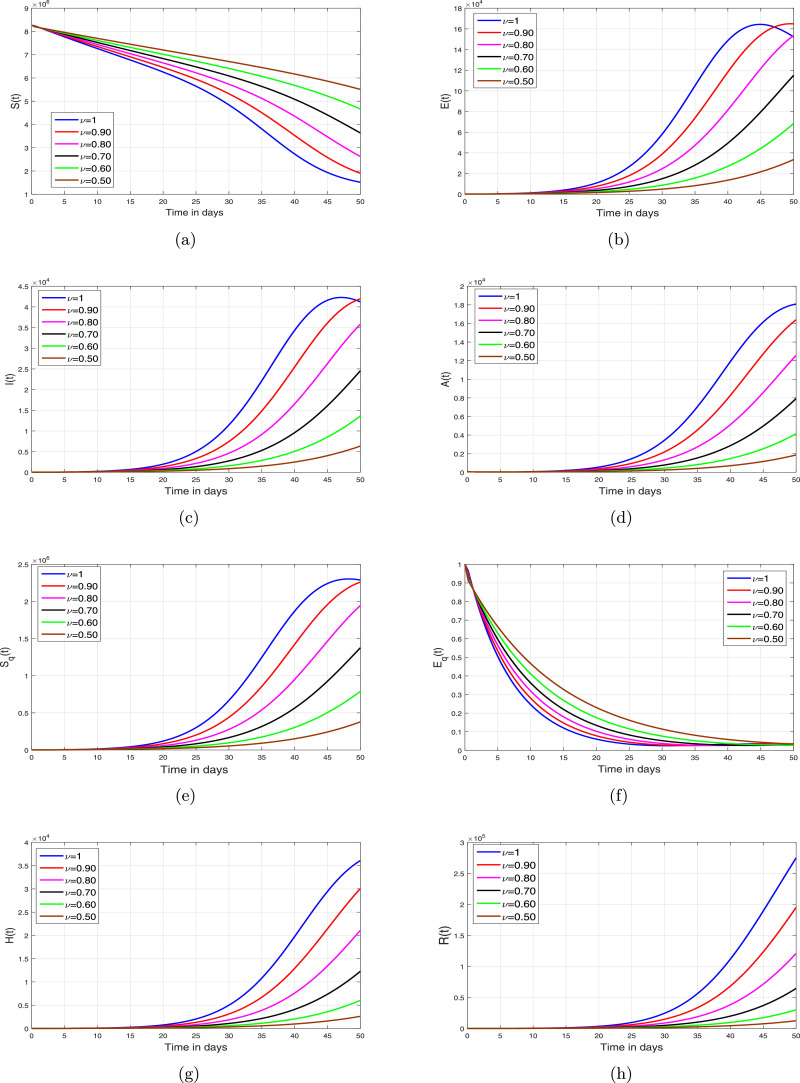
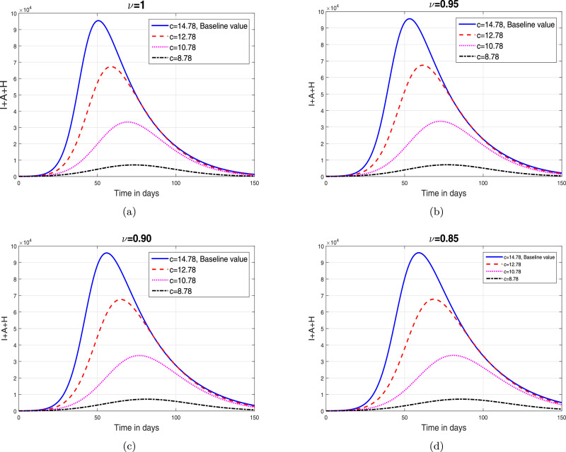
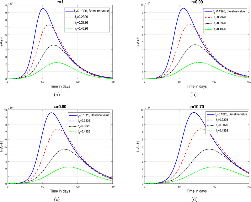
Based on the iterative scheme (34) and (35), we present some simulation results in order to analyze the impact of fractional oreide on disease dynamics. The resulting simulations are depicted in Fig. 2, Fig. 3, Fig. 4, Fig. 5 .

Fig. 2.

Simulations of the COVID-19 model (8) for different values of fractional order $\nu$.

Fig. 3.

The impact of parameter $c$ (contact rate) on total infective population where (a) $\nu =1,$ (b) $\nu =0.9,$ (c) $\nu =0.8,$ (d) $\nu =0.7$.

Fig. 4.

The impact of parameter ${\delta }_I$ (isolation rate) on total infective population where (a) $\nu =1,$ (b) $\nu =0.9,$ (c) $\nu =0.8,$ (d) $\nu =0.7$.

Fig. 5.

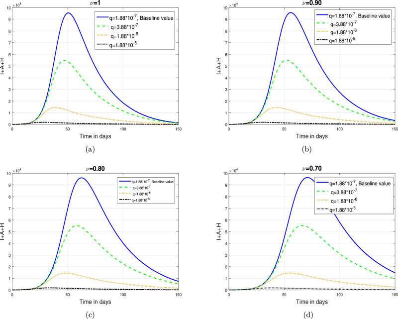
The impact of parameter $q$ (quarantine rate) on total infective population where (a) $\nu =1,$ (b) $\nu =0.9,$ (c) $\nu =0.8,$ (d) $\nu =0.7$.

5.1. Discussion

In this section, we depict the simulation results using an iterative scheme developed in the previous section. The purpose of the graphical results is to explore the possible impact of memory index and enhancement in various interventions like contact rate, hospitalization/isolation and quarantine on disease dynamics. The parameter values given in Table 1 are used to obtain the Fig. 2, Fig. 3, Fig. 4, Fig. 5. These graphical interpretations reveal that the non integer order derivative has a significant impact on the dynamics of the epidemic. In Fig. 2, we analyze the variation in the dynamical behavior of model variables for different values of the fractional order $\nu$ of CF operator. It can be observed that the symptomatic, asymptomatic and hospitalized infected individuals are decreased when we decrease $\nu$. The impact of contact rate denoted by $c$ on the total symptomatic, asymptomatic and hospitalized COVID-19 infective population is depicted in Fig. 3. We have shown this interpretation for four different value of $\nu$ as can be found in subplots 3(a)–(d). This analysis shows that when the contact rate $c$ is decreasing, the peaks of infective population decreases significantly. The same behavior is observed for all values of $\nu$. The impact of isolation rate ${\delta }_I$ on cumulative symptomatic, asymptomatic and hospitalized COVID-19 infective population is observed in Fig. 4 with subplots (a)–(d). With the increase in the hospitalization/isolation rate a reasonable decrease in the pandemic peaks is observed. Almost the same effect is found for all values of $\nu$. Finally, the impact of enhancement in quarantine rate (after contact tracing) is demonstrated in Fig. 5. This analysis shows that the enhancement of quarantine rate can significantly reduce the pandemic peak and decrease the cumulative number of predicted reported COVID-19 infected cases as can be seen in 5(a)–(d).

6. Conclusion

The novel COVID-19 pandemic is a huge panic for human health and economy. Although most of the countries overcome this infection still much research is needed to explore the complex transmission dynamics of COVID-19. In this paper, we have reformulated the mathematical model for the dynamic of COVID-19 virus studied in Tang et al. [6] under the Caputo–Fabrizio fractional derivatives with an exponential kernel in order to capture the memory effects. The positivity and the boundedness of solutions are proven. Moreover, by using Banach fixed point theory we have established the existence and uniqueness of the solution of fractional COVID-19 model (9). An efficient iterative scheme is applied to derived the numerical solution of the fractional model. Many simulations are depicted and discussed for various values of fractional order describing the role of different interventions in the disease eradication. The present investigations revealed that the reduction in the contact rate $c$ and enhancing the contact-tracing policy to quarantine the exposed individuals significantly reduced the peak of infected curves. Moreover, the decrease in the infected population becomes more significant for smaller values of fractional order. These graphical interpretations demonstrate the importance of memory index and thus, we conclude that the epidemic models with fractional operator can be used to gain more insights about a disease dynamics.

Credit author statement

All authors contributed to the present manuscript.

Declaration of Competing Interest

The authors declare that they have no known competing financial interests or personal relationships that could have appeared to influence the work reported in this paper.

References

- 1.World Health Organization. https://www.who.int/emergencies/diseases/novel-coronavirus-2019. Accessed 30th June 2020.
- 2.Center for Disease Control, Prevention (CDC). https://www.cdc.gov/coronavirus/2019-ncov/index.html
- 3.Fanelli D., Piazza F. Analysis and forecast of COVID-19 spreading in China, Iitaly and France. Chaos Solitons Fractals. 2020;134:109761. doi: 10.1016/j.chaos.2020.109761. [DOI] [PMC free article] [PubMed] [Google Scholar]
- 4.Asamoah J.K.K., Owusu M., Jin Z., Oduro F., Abidemi A., Gyasi E.O. Global stability and cost-effectiveness analysis of COVID-19 considering the impact of the environment: using data from Ghana. Chaos Solitons Fractals. 2020;140:110103. doi: 10.1016/j.chaos.2020.110103. [DOI] [PMC free article] [PubMed] [Google Scholar]
- 5.Ullah S., Khan M.A. Modeling the impact of non-pharmaceutical interventions on the dynamics of novel coronavirus with optimal control analysis with a case study. Chaos Solitons Fractals. 2020;139:110075. doi: 10.1016/j.chaos.2020.110075. [DOI] [PMC free article] [PubMed] [Google Scholar]
- 6.Tang B., Wang X., Li Q., Bragazzi N.L., Tang S., Xiao Y., et al. Estimation of the transmission risk of the 2019-nCoVand its implication for public health interventions. J Clin Med. 2020;9(462):1–13. doi: 10.3390/jcm9020462. [DOI] [PMC free article] [PubMed] [Google Scholar]
- 7.Khan M.A., Azizah M., Ullah S., et al. A fractional model for the dynamics of competition between commercial and rural banks in Indonesia. Chaos Solitons Fractals. 2019;122:32–46. [Google Scholar]
- 8.Ullah S., Khan M.A., Farooq M. A fractional model for the dynamics of TB virus. Chaos Solitons Fractals. 2018;116:63–71. [Google Scholar]
- 9.Baleanu D., Jajarmi A., Bonyah E., Hajipour M. New aspects of poor nutrition in the life cycle within the fractional calculus. Adv Differ Equ. 2018;2018(1):1–14. [Google Scholar]
- 10.Danane J., Allali K., Hammouch Z. Mathematical analysis of a fractional differential model of HBV infection with antibody immune response. Chaos Solitons Fractals. 2020;136:109787. [Google Scholar]
- 11.Atangana A., Baleanu D. New fractional derivatives with nonlocal and non-singular kernel: theory and application to heat transfer model. Therm Sci. 2016;20(2):763–769. [Google Scholar]
- 12.Podlubny I. Elsevier; 1998. Fractional differential equations: an introduction to fractional derivatives, fractional differential equations, to methods of their solution and some of their applications. [Google Scholar]
- 13.Caputo M., Fabrizio M. A new definition of fractional derivative without singular kernel. Prog Fract DifferAppl. 2015;1(2):73–85. [Google Scholar]
- 14.Baleanu D., Khan M.A., Hammouch Z.. Modeling the dynamics of hepatitis via the Caputo–Fabrizio derivative2019.
- 15.Ullah S., Khan M.A., Farooq M., Hammouch Z., Baleanu D. A fractional model for the dynamics of tuberculosis infection using Caputo–Fabrizio derevative. Discrete Contin Dyn Syst Ser S. 2020;13(3):975–993. [Google Scholar]
- 16.Ullah S., Khan M.A., Farooq M. A new fractional model for the dynamics of the hepatitis B virus using the Caputo–Fabrizio derivative. Eur Phys J Plus. 2018;133(6):237. [Google Scholar]
- 17.Baleanu D., Mohammadi H., Rezapour S. A fractional differential equation model for the COVID-19 transmission by using the Caputo–Fabrizio derivative. Adv Differ Equ. 2020;2020(1):1–27. doi: 10.1186/s13662-020-02762-2. [DOI] [PMC free article] [PubMed] [Google Scholar]
- 18.Atangana A. Modelling the spread of COVID-19 with new fractal-fractional operators: can the lockdown save mankind before vaccination? Chaos Solitons Fractals. 2020;136:109860. doi: 10.1016/j.chaos.2020.109860. [DOI] [PMC free article] [PubMed] [Google Scholar]
- 19.Khan M.A., Atangana A. Modeling the dynamics of novel coronavirus (2019-nCoV) with fractional derivative. Alexandria Eng J. 2020;59(4):2379–2389. [Google Scholar]
- 20.Losada J., Nieto J.J. Propreties of a new fractional derivative without singular kernel. Prog Fract DifferAppl. 2015;1(2):87–92. [Google Scholar]
- 21.China Population 1950–2020. https://www.worldometers.info/world-population/china-population/.
- 22.Atangana A., Owolabi K.M. New numerical approach for fractional differential equations. Math Model Natural Phenomena. 2018;13(1):3. [Google Scholar]
- 23.Owolabi K.M., Atangana A. Analysis and application of new fractional Adams–Bashforth scheme with Caputo–Fabrizio derivative. Chaos Solitons Fractals. 2017;105:111–119. [Google Scholar]