

Abstract
Ovarian cancer is a heterogeneous disease at the molecular and histologic level. Optical coherence tomography (OCT) is able to map ovarian tissue optical properties and heterogeneity, which has been proposed as a feature to aid in diagnosis of ovarian cancer. In this manuscript, depth-resolved en face scattering maps of malignant ovaries, benign ovaries, and benign fallopian tubes obtained from 20 patients are provided to visualize the heterogeneity of ovarian tissues. Six features are extracted from histograms of scattering maps. All features are able to statistically distinguish benign from malignant ovaries. Two prediction models were constructed based on these features: a logistic regression model (LR) and a support vector machine (SVM). The optimal set of features is mean scattering coefficient and scattering map entropy. The LR achieved a sensitivity and specificity of 97.0% and 97.8%, and SVM demonstrated a sensitivity and specificity of 99.6% and 96.4%. Our initial results demonstrate the feasibility of using OCT as an “optical biopsy tool” for detecting the microscopic scattering changes associated with neoplasia in human ovarian tissue.
Keywords: cancer prediction, optical coherence tomography, ovarian cancer, scattering coefficient map
Graphical Abstract
1 |. INTRODUCTION
Ovarian cancer is the fifth leading cause of cancer death among women and the most lethal gynecologic cancer [1, 2]. The 5-year survival rate of ovarian cancer is only 40% due to late detection [3]. However, when diagnosed at stage I, ovarian cancer has a 5-year survival rate of 92% [1]. Currently the best screening method provided for women at high risk is a CA125 blood test combined with transvaginal ultrasound; unfortunately, the sensitivity and specificity are low and only 15% of ovarian cancers are diagnosed at an early stage [4]. The standard of care for high-risk women is risk-reducing bilateral salpingo-oophorectomy (RRSO), which can reduce the risk of ovarian cancer by more than 50% [5, 6]. However, RRSO causes early menopause, which carries risks, including accelerated bone loss and increased risk of heart disease [7].
Ovarian cancer is a heterogeneous disease at the molecular and histologic level [8, 9]. During the progression of ovarian cancer, the collagen fiber architecture of the extracellular matrix is remodeled [10, 11]. As collagen fibers are the main elastic scatterers in the ovarian stroma, the redistribution and re-organization of collagen fiber bundles affect its optical scattering properties. A noninvasive and sensitive micrometer-resolution instrument has the potential to identify these structural alterations for early detection of ovarian cancer.
Optical coherence tomography (OCT) can provide microscale real-time images and is able to obtain an “optical biopsy” without physically resecting the tissue [12–15]. The OCT contrast is generated from the backscattered light from different layers of tissue; thus, it is suitable for extracting tissue scattering heterogeneity. The feasibility of OCT in laparoscopy and falloposcopy for ovarian tissue B-scan imaging has already been demonstrated [16, 17]. The scattering coefficient, which is related to the collagen content and directivity, was extracted from OCT A-scans and found to be a good biomarker for characterizing human ovarian cancer [18, 19]. Scattering coefficient distribution within B-scans based on 2-D analysis and histogram analysis of B-scan images have been used in automated classification of urinary bladder cancer, Barrett’s esophagus, human skin cancer, and human atrial tissue using OCT. [20–23] All these studies mainly focus on B-scan images and features, and show promising results. 3-D texture analysis of OCT images of a mouse ovary model achieved statistically significant performance [24]. Histogram analysis has also been applied to MRI, ultrasound, and CT to characterize tumor heterogeneity [25–27]. Spatial frequency domain imaging (SFDI) is another imaging modality that is able to quantify scattering and has shown promise in classifying ovarian tissue [28]. SFDI has a large field of view; however, its resolution (~mm) is not high enough to detect neoplastic microstructural scatter changes associated with the progression of ovarian cancer.
In this study, we report, for the first time, characterization and classification of ex vivo human ovary and fallopian tube based on features obtained from 3-D analysis of depth-resolved en face scattering maps of OCT images. Initial results indicate that quantitative scattering features extracted from the OCT images can be used to identify ovarian cancer.
2 |. MATERIALS AND METHODS
2.1 |. Ovary sample preparation
This study was approved by the Institutional Review Board (IRB), and informed consent was obtained from all patients. A total of 26 freshly excised human ovaries and 9 fallopian tubes from 20 patients (see Table 1) undergoing surgery for various clinical indications were imaged with OCT in the Optical and Ultrasound Imaging Lab located at Washington University School of Medicine. Ovaries were imaged immediately after surgery (~5 mins) and returned to the Pathology Department within an hour for routine processing. Pathologists in the frozen section lab provided guidance to the researchers as to the sample orientation and location of tumor, which was in any event not subtle. Therefore, we are certain that we imaged the tumor for the malignant specimens.
TABLE 1.
Lesion characteristics (20 patients of 26 ovaries, average age 56 years; range 37–87)
| Cancerous ovaries | High grade serous carcinoma (n = 4, average size 8 cm, range 5.5–10 cm) |
| Sertoli-Leydig cell tumor (n = 1, size 19.2 cm) | |
| Benign ovaries | Fibrothecoma (n = 1, size 14 cm) |
| Cystic follicles (n = 1, size 3 cm) | |
| Epidermoid cyst (n = 1, size 7.6 cm) | |
| Inclusion cysts (n = 2, average size 4.3 cm, range 3.5–5 cm) | |
| Mesothelial cyst (n = 1, size 3.1 cm) | |
| Cortical, fibrosis, and hyperthecosis hemorrhagic corpus luteum (n = 1, size 4 cm) | |
| Benign leiomyoma (n = 1, size 5.5 cm) | |
| Serous/Mucinous cystadenoma (n = 6, average size 8.4 cm, range 2.5–21 cm) | |
| Benign cystic endometriosis (n = 1, size 6 cm) | |
| No significant histopathological abnormalities (n = 6) | |
| Benign fallopian tubes | No significant histopathological abnormalities (n = 9) |
2.2 |. Swept-source OCT system and experimental design
The OCT system is based on a swept source (HSL-2000, Santec Corp., Japan) with a center wavelength of 1310 nm, a FWHM bandwidth of 110 nm, and a scan rate of 20 kHz. The interference signal was detected by a balanced detector (Thorlabs PDB450C) and acquired by an A/D card (ATS9462, AlazarTech Technologies Inc). The lateral resolution of the system in the air is 10 μm, and the axial resolution is 6 μm. To compensate for system signal-to-noise ratio roll-off and Gaussian beam focusing, a calibration test was performed by measuring attenuated mirror signals from different imaging depths. For each 3-D scan of an ovarian tissue sample, an area of 5 mm × 10 mm was scanned. An illustration of the experimental setup and imaging system can be found in our recent publication [29].
2.3 |. Feature extraction
2.3.1 |. Generating en face scattering coefficient maps
For ovarian specimens, collagen fibers were found to be the main scattering source in the stroma underlying the surface epithelium [30–32]. Thus, the ovarian epithelium layer was first located semi-automatically (area between the two red curves in Figure 1A,C) using the shortest-path algorithm [33]. A wavelet filter was applied to B-scan images for noise reduction and fitting [33]. Then the scattering coefficient within the ovarian cortex layer was calculated by fitting each A-scan with a single scattering model based on Beer’s law [34, 35]. By fitting all A-lines within one 3-D scan (1000 A-lines × 500 B-scans), we generated a depth-resolved en face scattering coefficient map of the scanned ovarian tissue.
FIGURE 1.

Representative OCT images of benign and malignant ovary specimens. The ovarian surface epithelium is between the two red curves in the B-scan SS-OCT images. (A) representative B-scan image from a benign ovary and (B) corresponding H&E image. (C) representative B-scan image from a malignant ovary (high-grade serous carcinoma) and (D) corresponding H&E image. Inset: best-fit Beer’s law is used to calculate the scattering coefficient. OCT, optical coherence tomography
2.3.2 |. Histogram feature extraction
Each scattering map was further subdivided into several nonoverlapping images to avoid hyper-reflection and out-of-focus areas. Six features were extracted quantitatively using MATLAB R2018a from the analysis of the histogram of all scattering maps. Six features can be computed from Eq. (1) to (6), where xi is the pixel gray level and N is the total number of pixels.
| (1) |
| (2) |
| (3) |
| (4) |
| (5) |
| (6) |
Where s(1) is the image width and s(2) is the image length. The statistical significance of these six features was further evaluated using the Wilcoxon ranksum test.
2.4 |. Feature selection and classification
In the first step, the Spearman’s cross correlation among all features was evaluated (Table 2) and features with correlation coefficient smaller than 0.5 were considered independent of each other [36, 37]. Next, two optimal feature sets: “mean and entropy” and “energy, skewness, entropy” were selected. Each optimal feature set consists of features that are not correlated by our measure and provide best testing results [38]. Then two prediction models (LR and SVM) were trained using these two feature sets through glmfit and fitcsvm functions in MATLAB. Approximately two thirds of the data were used for training two predictive classifiers and the rest were used for testing the models. Repeated rounds (100 times) of training and testing were applied by randomly selecting 2/3 of the samples for training and 1/3 of the samples for testing. One hundred receiver operating curves (ROC) were generated, and the averaged sensitivity, specificity, and area under the curve (AUC) were used for evaluating the accuracy of the model.
TABLE 2.
Spearman’s cross correlation between each pair of features proposed for distinguishing benign ovarian specimens from malignant. Features with ρ <0.5 were considered independent
| Mean | Variance | Entropy | Skewness | Kurtosis | Energy | |
|---|---|---|---|---|---|---|
| Mean | 1 | 0.81 | 0.35 | 0.73 | 0.87 | 0.55 |
| Variance | 1 | 0.37 | 0.44 | 0.86 | 0.85 | |
| Entropy | 1 | 0.09 | 0.23 | 0.09 | ||
| Skewness | 1 | 0.72 | 0.37 | |||
| Kurtosis | 1 | 0.73 | ||||
| Energy | 1 |
3 |. RESULTS
A total of 20 patients (mean age 56 years; range 37–87) of 26 ovaries were imaged ex vivo from February 2017 to October 2018. Table 1 provides pathological characteristics of these ovaries. Diagnoses ascertained by subsequent surgical pathology examination revealed high-grade serous carcinoma (n = 4 ovaries), Sertoli-Leydig cell tumor (a sex cord-stromal tumor; n = 1), normal ovaries (n = 6), other causes of benign but enlarged ovaries (n = 15), and benign fallopian tubes (n = 9) (Table 1).
3.1 |. B-scan images of ovary samples
Representative SS-OCT B-scan images of benign ovaries, malignant ovaries, and corresponding H&E slides are shown in Figure 1. The OCT and the histologic images have similar scales and come from similar, but not identical, locations within the ovary specimens. In Figure 1B, non-neoplastic ovarian stroma is seen, characterized by bland spindle cells in a dense collagenous background. Figure 1D, in contrast, is infiltrated by high-grade serous carcinoma. Irregular islands of neoplastic cells are present in the lower left of the panel, characterized by increased nuclear to cytoplasmic ratio, formation of abortive glandular structures, and surrounding stromal desmoplasia (stromal reaction to invasive tumor). The neoplastic cellularity in this case is approximately 20% by visual estimate of the H&E slide, which is typical of cases included in the study.
3.2 |. Scattering coefficient maps of human ovary specimens
Figure 2A–C shows photographs of one benign ovary, one malignant ovary (high-grade serous carcinoma), and one benign fallopian tube, respectively. The scattering coefficient maps of the scanned areas, identified as white boxes in Figure 2A–C, are shown in Figure 2D–F. The white areas in the scattering map indicate the background or tissue area that is out of focus. The normal ovarian specimen exhibits much higher scattering on average and is more homogeneous compared to malignant ovary, which has significantly lower scatter and disorganized collagen distribution. The benign fallopian tube shows a spatially heterogeneous scattering distribution that significantly differs from the ovary scattering maps.
FIGURE 2.
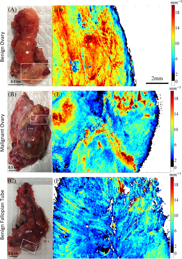
Photographs (A-C) of one benign ovary, one malignant ovary, and one benign fallopian tube, respectively. Scattering coefficient maps (D-F) of the scanned areas, identified as white boxes in Figure (A-C). The scale bar of 200 mm is shared by maps (D-F)
3.3 |. Histogram analysis
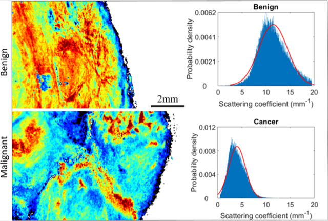
Six features were extracted from scattering maps and histograms of 27 nonoverlapping malignant ovary scattering maps, 64 nonoverlapping benign/normal ovary scattering maps, and 9 nonoverlapping benign fallopian tube scattering maps. Each nonoverlapping scattering map was from a 5 mm × 10 mm area of a different region of the examined ovary. Depending on the size of the ovary, one to four nonoverlapping areas were imaged and scattering maps were generated. Figure 3 shows representative histograms derived from one malignant ovary (Figure 3A) and one benign ovary (Figure 3B). The six features for Figure 3A are 4.0 mm−1 (mean), 1.71 (variance), 6.50 (entropy), 0.77 (skewness), 4.33 (kurtosis), and 0.17 (energy). The six features for Figure 3B are 11.48 mm−1(mean), 2.98 (variance), 7.30 (entropy), 0.22 (skewness), 2.85 (kurtosis), and 0.10 (energy). Gaussian curves (best-fit) of the histograms are shown in red for visualization. More details can be found in Table 3.
FIGURE 3.

Histogram analysis of one representative malignant ovary (A) and one representative benign ovary (B). The six features for (A) are 4.0 mm−1(mean), 1.71(variance), 6.50(entropy), 0.77(skewness), 4.33(kurtosis), and 0.17(energy). The six features for (B) are 11.48mm−1(mean), 2.98(variance), 7.30(entropy), 0.22(skewness), 2.85(kurtosis), and 0.10(energy). Fitted Gaussian distribution is shown as red curves
TABLE 3.
Scattering coefficient map’s histogram features (mean ±SD) of ovarian tissues
| Mean(mm−1) | Variance | Entropy | Skewness | Kurtosis | Energy | |
|---|---|---|---|---|---|---|
| Cancer Ovary | 4.4 ± 1.0 | 1.9 ± 0.5 | 6.7 ± 0.3 | 0.6 ± 0.2 | 3.0 ± 0.1 | 0.085 ± 0.005 |
| Benign Ovary | 9.1 ± 1.6 | 3.8 ± 0.6 | 7.2 ± 0.4 | 0.4 ± 0.2 | 2.6 ± 0.3 | 0.078 ± 0.008 |
| Benign Tubes | 6.4 ± 1.9 | 2.8 ± 0.9 | 7.1 ± 0.4 | 0.5 ± 0.1 | 2.8 ± 0.2 | 0.083 ± 0.006 |
Figure 4 shows the boxplots for the mean, variance, entropy, skewness, kurtosis, and energy across the entire set of 26 ovaries. All features showed statistically significant differences between malignant and benign ovarian tissues. Cancerous specimens had significantly lower mean, variance, and entropy of scattering coefficient, but markedly higher skewness, kurtosis, and energy than benign specimens. The mean and variance were significantly different between cancer ovaries and benign fallopian tubes, and the mean, variance, and kurtosis had statistically significant differences between benign ovaries and benign fallopian tubes. In addition, fallopian tubes showed different scatter distribution than either malignant tissue or benign tissue.
FIGURE 4.

Boxplot of the six features extracted from histogram analysis of scattering maps of malignant ovaries, benign ovaries, and benign fallopian tubes
3.4 |. Training and testing results of two predictive models
Although all features differed between benign and malignant, we hypothesized that a combination of features would allow better classification of ovaries. Figure 5 shows ROC curves for the testing sets of both LR and SVM models trained on two optimal feature sets. The first feature set consisted of mean scattering coefficient and scattering map entropy. For this set, a sensitivity and specificity of 97.0% and 97.8% was obtained from LR, with average AUC of 0.986; a sensitivity and specificity of 99.6% and 96.4% was achieved from the SVM, with average AUC of 0.991. A second set consisted of energy, skewness, and entropy. The trained LR model achieved a sensitivity and specificity of 93.4% and 82.1%, with average AUC of 0.956; the SVM achieved a sensitivity and specificity of 91.1% and 84.2%, with average AUC of 0.957. Thus, the optimal set of features is mean scattering coefficient and scattering map entropy. Both LR and SVM have similar diagnostic performance.
FIGURE 5.

Testing results of two optimal data sets ([mean, entropy] and [energy, skewness, entropy]) used to train two classification models. (A-B) show the ROC curves for the testing sets of logistic regression and (C-D) show the ROC curves of SVM model
4 |. DISCUSSION
In this study, depth-resolved human ovary and fallopian tube en face scattering coefficient maps are presented for the first time. The scattering coefficient map of malignant and benign ovarian tissues shows differences attributed to the presence of malignancy. Benign ovarian tissue demonstrated a homogeneous scatter distribution with high average scattering coefficient. Malignant ovarian tissues were heterogeneous with generally lower subsurface scattering coefficient. The difference between the scattering properties of the samples can be attributed to the reorganization of collagen in the ovarian tissue, although we did not directly test this. When cancer develops in healthy ovaries, it invades the collagen network and causes the remodeling of collagen architecture [10, 11]. This results in the heterogeneous distribution seen in Figure 2E.
In addition, we can summarize the scattering coefficient maps by calculating mean, variance, entropy, skewness, kurtosis, and energy, which statistically separate benign from malignant tissues (Figure 4). Both LR and SVM models were trained based on these histogram features and achieved a high sensitivity, specificity, and AUC in testing. These interesting results indicate that OCT may be possible to predict the risk of cancer before surgery, which could potentially aid in clinical decision-making (eg, prioritizing surgical cases with higher risk of malignancy, avoiding unnecessary resection of low-risk cases, or triaging patients for referral to a gynecologic oncologist). It is worth to mention that the training and testing datasets are small (60 for training and 30 for testing), and overfitting can occur when the training dataset is limited [39]. We have selected the minimal number of independent predictors (one optimal set has three parameters, and second has two parameters) for each prediction tests, performed 100 times cross-validation, and used fairly high amounts (33%) of the sample data for testing. The performances of the prediction models based on respective training and testing datasets are similar with no obvious pattern of higher AUC values for training data and much lower AUCs for testing data, which would be expected if there were problem of overfitting. With more patients recruited to the study, we will be able to establish a large database to validate prediction models with more input predictors.
The malignant cases reported in this study were at various stages including stage I (for the Sertoli-Leydig cell tumor), stage II (one high-grade serous cancer) and stage III (three high-grade serous cancers). Thus, a range of stages was represented. The progression from stage I to IV, based on the definitions of the International Federation of Gynecology and Obstetrics, does not necessarily involve more extensive involvement of the ovary, but rather is based on involvement of remote sites in the pelvis (stage II), abdomen (stage III) or elsewhere (stage IV). Therefore, one would not a priori expect the imaging characteristics of stage I ovarian cancers to differ from those of more advanced cases; the ovary could be involved to the same extent in any of these stages. The volume of cancer in an ovary may range from small to large, and it is plausible that the scattering maps of ovarian cancer tissue might vary depending on the size of the tumors. Our tumors did range from 5.5 to 10 cm in diameter (Table 1). It might be desirable to explore the operating characteristics of the imaging over a wider range of sizes. We would underline that this was a proof of principle study intended to document the imaging characteristics of benign as compared to malignant tissue. Once these characteristics are known, they can then be applied to ambiguous or difficult cases. It will eventually be important to determine the sensitivity and specificity of the OCT technique in a real-world mix of cases, including early-stage and small cases. Ovarian cancer is usually detected at advanced stage, and is often clinically “silent” until the tumor reaches a large size. It is therefore not surprising that our relatively small sample of convenience consisted of larger tumors.
Our study provides evidence that the benign fallopian tubes demonstrate different microscopic scattering distribution as compared to ovarian tissues. We have made the assumption that benign entities can be considered together (regardless of specific histologic diagnosis) and that malignant entities can be considered together, an assumption that is supported by the homogeneity of features in each group, as shown in Figure 4. A limitation of our study is the lack of malignant fallopian tubes. Studies have shown that the fallopian tube is the origin of high-grade serous carcinoma, which is the most common and most lethal subtype of ovarian cancer [40–42]. Keenan et al. provided B-scan images using an OCT falloposcope imaging porcine fallopian tubes, presumably benign [17]. Madore et al. showed B-scan images of a fresh excised healthy human fallopian tube [43]. These studies focus on proving the feasibility of falloposcope and providing qualitative OCT images. Our future work will be focused on quantitative discrimination of microscopic scattering changes in benign and malignant fallopian tubes. Because malignant fallopian tubes are rare, a larger scale clinical study is needed.
A limitation of this study is that we have studied only the most common pathologic entities to occur in the ovary. A real-world mix of patients will include a larger spectrum of diagnoses, including tumors of other epithelial cell types, borderline tumors, sex cord-stromal tumors, germ cell tumors, metastatic tumors, and benign processes that enlarge the ovary such as tubo-ovarian abscess and endometriosis. Some more complicated cases will be included in future studies, including but not limited to specimens with a mixture of pathologies and ovaries with subtle involvement. Moving forward, one critical obstacle for translating OCT into in vivo imaging as a clinical screening technique will be data acquisition. As ovaries are deeply buried within the human abdomen, it is challenging to access them. Several approaches have been proposed so far, including OCT laparoscopy [16] and falloposcopy [17]. Future studies will focus on endoscopic OCT designs and evaluate them in vivo.
Currently, all image post-processing is performed in MATLAB. The total image post-processing time for a 5 mm by 1 cm (500 B-scans, 1000 A-lines/B-scan, and 1024 pixels/A-line) area is 12 hours on a Dell Inspiron 3650 (64 bits, Intel Core i5–6400 CPU @ 2.70GHz, 8GB RAM), which is too long for real-time decision-making. Future work will need to focus on algorithm optimization for faster and more accurate surface delineation and scattering coefficient fitting, and on GPU implementation for improving computational speed. Certainly, an automatic scattering coefficient map segmentation algorithm is needed for real-time data processing. Many automatic segmentation algorithms for OCT images have been implemented [44], for example, feature-based segmentation and machine learning based methods. A suitable methodology will be thoroughly explored in the future. The final goal is to provide real-time quantitative assessment of microscopic optical scattering changes associated with development and progression of ovarian cancers.
Supplementary Material
ACKNOWLEDGMENTS
The authors acknowledge the funding support of NCI (R01CA151570). The authors would like to thank Ruth Holdener from the Mallinckrodt Institute of Radiology and Lynne Lippmann from the Division of Gynecologic Oncology at Washington University School of Medicine for helping with patient consent and study coordination.
Funding information
National Cancer Institute, Grant/Award Number: R01CA151570
Footnotes
AUTHOR BIOGRAPHIES
Please see Supporting Information online.
REFERENCES
- [1].Siegel RL, Miller KD, Jemal A, CA Cancer J. Clin. 2019, 69 (1), 7. [DOI] [PubMed] [Google Scholar]
- [2].Nandy S, Mostafa A, Hagemann IS, Powell MA, Amidi E, Robinson K, Mutch DG, Siegel C, Zhu Q, Radiology 2019, 289(3), 740. [DOI] [PMC free article] [PubMed] [Google Scholar]
- [3].Torre LA, Trabert B, DeSantis CE, Miller KD, Samimi G, Runowicz CD, Gaudet MM, Jemal A, Siegel RL, CA Cancer J. Clin. 2018, 68(4), 284. [DOI] [PMC free article] [PubMed] [Google Scholar]
- [4].van Nagell JR Jr, DePriest PD, Reedy MB, Gallion HH, Ueland FR, Pavlik EJ, Kryscio RJ, Gynecol. Oncologia 2000, 77(3), 350. [DOI] [PubMed] [Google Scholar]
- [5].Rebbeck TR, Lynch HT, Neuhausen SL, Narod SA, van’t Veer L, Garber JE, Evans G, Isaacs C, Daly MB, Matloff E, Olopade OI, Weber BL, N. Engl. J. Med. 2002, 346(21), 1616. [DOI] [PubMed] [Google Scholar]
- [6].Kauff ND, Satagopan JM, Robson ME, Scheuer L, Hensley M, Hudis CA, Ellis NA, Boyd J, Borgen PI, Barakat RR, Norton L, Castiel M, N. Engl. J. Med. 2002, 346 (21), 1609. [DOI] [PubMed] [Google Scholar]
- [7].Parker WH, Broder MS, Chang E, Feskanich D, Farquhar C, Liu Z, Shoupe D, Berek JS, Hankinson S, Manson JE, Obstet. Gynecol. 2009, 113(5), 1027. [DOI] [PMC free article] [PubMed] [Google Scholar]
- [8].Bowtell DDL, Nat. Rev. Cancer 2010, 10(11), 803. [DOI] [PubMed] [Google Scholar]
- [9].Prat J, Ann. Oncol 2012, 23(Suppl 10), 111. [DOI] [PubMed] [Google Scholar]
- [10].Arifler D, Pavlova I, Gillenwater A, Richards-Kortum R, Biophys. J. 2007, 92(9), 3260. [DOI] [PMC free article] [PubMed] [Google Scholar]
- [11].Nandy S, Salehi HS, Wang T, Wang X, Sanders M, Kueck A, Brewer M, Zhu Q, Biomed. Opt. Express 2015, 6(10), 3806. [DOI] [PMC free article] [PubMed] [Google Scholar]
- [12].Huang D, Swanson EA, Lin CP, Schuman JS, Stinson WG, Chang W, Hee MR, Flotte T, Gregory K, Puliafito CA, Fujimoto JG, Science 1991, 254 (5035), 1178. [DOI] [PMC free article] [PubMed] [Google Scholar]
- [13].Tearney GJ, Brezinski ME, Bouma BE, Boppart SA, Pitris C, Southern JF, Fujimoto JG, Science 1997, 276(5321), 2037. [DOI] [PubMed] [Google Scholar]
- [14].Bouma BE, Yun S, Vakoc BJ, Suter MJ, Tearney GJ, Curr. Opin. Biotechnol. 2009, 20(1), 111. [DOI] [PMC free article] [PubMed] [Google Scholar]
- [15].Wang T, Xie L, Huang H, Li X, Wang R, Yang G, Du Y, Huang G, Chin. Opt. Lett. 2013, 11(11), 111102. [Google Scholar]
- [16].Boppart SA, Goodman A, Libus J, Pitris C, Jesser CA, Brezinski ME, Fujimoto JG, Br. J. Obstet. Gynaecol. 1999, 106(10), 1071. [DOI] [PubMed] [Google Scholar]
- [17].Keenan M, Tate TH, Kieu K, Black JF, Utzinger U, Barton JK, Biomed. Opt. Express 2017, 8(1), 124. [DOI] [PMC free article] [PubMed] [Google Scholar]
- [18].Yang Y, Wang T, Biswal NC, Wang X, Sanders M, Brewer M, Zhu Q, J. Biomed. Opt 2011, 16(9), 090504. [DOI] [PMC free article] [PubMed] [Google Scholar]
- [19].Wang T, Yang Y, Zhu Q, Biomed. Opt. Express 2013, 4 (5), 772. [DOI] [PMC free article] [PubMed] [Google Scholar]
- [20].Lingley-Papadopoulos CA, Loew MH, Manyak MJ, Zara JM, J. Biomed. Opt. 2008, 13(2), 024003. [DOI] [PubMed] [Google Scholar]
- [21].Qi X, Sivak MV, Isenberg G, Willis JE, Rollins AM, J. Biomed. Opt 2006, 11(4), 044010. [DOI] [PubMed] [Google Scholar]
- [22].Marvdashti T, Duan L, Aasi SZ, Tang JY, Ellerbee Bowden AK, Biomed. Opt. Express 2016, 7(9), 3721. [DOI] [PMC free article] [PubMed] [Google Scholar]
- [23].Gan Y, Tsay D, Amir SB, Marboe CC, Hendon CP, J. Biomed. Opt. 2016, 21(10), 101407. [DOI] [PMC free article] [PubMed] [Google Scholar]
- [24].Sawyer TW, Chandra S, Rice PFS, Koevary JW, Barton JK, Phys. Med. Biol. 2018, 63(23), 235020. [DOI] [PMC free article] [PubMed] [Google Scholar]
- [25].Just N, Br. J. Cancer 2014, 111(12), 2205. [DOI] [PMC free article] [PubMed] [Google Scholar]
- [26].Sadeghi-Naini A, Papanicolau N, Falou O, Zubovits J, Dent R, Verma S, Trudeau M, Boileau JF, Spayne J, Iradji S, Sofroni E, Lee J, Lemon-Wong S, Yaffe M, Kolios MC, Czarnota GJ, Clin. Cancer Res. 2013, 19(8), 2163. [DOI] [PubMed] [Google Scholar]
- [27].Miles KA, Ganeshan B, Hayball MP, Cancer Imaging 2013, 13(3), 400. [DOI] [PMC free article] [PubMed] [Google Scholar]
- [28].Nandy S, Mostafa A, Kumavor PD, Sanders M, Brewer M, Zhu Q, J. Biomed. Opt. 2016, 21(10), 101402. [DOI] [PMC free article] [PubMed] [Google Scholar]
- [29].Zeng Y, Rao B, Nandy S, Hagemann I, Siegel C, Powell M, Zhu Q, Proc.SPIE 2018, 10483, 1048338. [Google Scholar]
- [30].Saidi IS, Jacques SL, Tittel FK, Appl. Opt. 1995, 34(31), 7410. [DOI] [PubMed] [Google Scholar]
- [31].Watson JM, Marion SL, Rice PF, Bentley DL, Besselsen DG, Utzinger U, Hoyer PB, Barton JK, Cancer Biol. Ther. 2014, 15(1), 42. [DOI] [PMC free article] [PubMed] [Google Scholar]
- [32].Wang T, Brewer M, Zhu Q, Wiley Interdiscip. Rev. 2015, 7 (1), 1. [DOI] [PMC free article] [PubMed] [Google Scholar]
- [33].Zeng Y, Rao B, Chapman WC Jr., Nandy S, Rais R, Gonzalez D. Chatterjee, Mutch M, Zhu Q, Sci. Rep. 2019, 9 (1), 2998. [DOI] [PMC free article] [PubMed] [Google Scholar]
- [34].Faber D, van der Meer F, Aalders M, van Leeuwen T, Opt. Express 2004, 12(19), 4353. [DOI] [PubMed] [Google Scholar]
- [35].Lee P, Gao W, Zhang X, Appl. Opt. 2010, 49(18), 3538. [DOI] [PubMed] [Google Scholar]
- [36].Hauke J, Kossowski T, Qua. Geo. 2011, 30(2), 87. [Google Scholar]
- [37].Amidi E, Mostafa A, Nandy S, Yang G, Middleton W, Siegel C, Zhu Q, Biomed. Opt. Express 2019, 10(5), 2303. [DOI] [PMC free article] [PubMed] [Google Scholar]
- [38].Guyon I, Elisseeff A, J. Mach. Learn. Res. 2003, 3(Mar), 1157. [Google Scholar]
- [39].Concato J, Feinstein AR, Holford TR, Ann. Intern. Med. 1993, 118(3), 201. [DOI] [PubMed] [Google Scholar]
- [40].Kurman RJ, Shih l M., Am. J. Surg. Pathol. 2010, 34(3), 433. [DOI] [PMC free article] [PubMed] [Google Scholar]
- [41].Erickson BK, Conner MG, Landen CN Jr., J. Am, Obstet. Gynecologie 2013, 209(5), 409. [DOI] [PMC free article] [PubMed] [Google Scholar]
- [42].George SH, Garcia R, Slomovitz BM, Front. Oncol. 2016, 6, 108. [DOI] [PMC free article] [PubMed] [Google Scholar]
- [43].Madore WJ, De Montigny E, Deschenes A, Benboujja F, Leduc M, Mes-Masson AM, Provencher DM, Rahimi K, Boudoux C, Godbout N, J. Biomed. Opt. 2017, 22(7), 76012. [DOI] [PubMed] [Google Scholar]
- [44].Sawyer TW, Rice PFS, Sawyer DM, Koevary JW, Barton JK, J. Med. Imaging 2019, 6(1), 014002. [DOI] [PMC free article] [PubMed] [Google Scholar]
Associated Data
This section collects any data citations, data availability statements, or supplementary materials included in this article.