QUANTIFYING ACTIN FILAMENTS IN MICROSCOPIC IMAGES USING KEYPOINT DETECTION TECHNIQUES AND A FAST MARCHING ALGORITHM

Abstract

The actin filament plays a fundamental role in numerous cellular processes such as cell growth, proliferation, migration, division, and locomotion. The actin cytoskeleton is highly dynamical and can polymerize and depolymerize in a very short time under different stimuli. To study the mechanics of actin filament, quantifying the length and number of actin filaments in each time frame of microscopic images is fundamental. In this paper, we adopt a Convolutional Neural Network (CNN) to segment actin filaments first, and then we utilize a modified Resnet to detect junctions and endpoints of filaments. With binary segmentation and detected keypoints, we apply a fast marching algorithm to obtain the number and length of each actin filament in microscopic images. We have also collected a dataset of 10 microscopic images of actin filaments to test our method. Our experiments show that our approach outperforms other existing approaches tackling this problem regarding both accuracy and inference time.

1. INTRODUCTION

In biological systems, there are many different filamentous structures playing essential roles in biological processes, and actin filaments are one of them. Actin filaments are abundant in all eukaryotic cells, and their functions are serving as tracks for a motor protein called myosin, highways inside cells for the transport of cargoes, motors for cell movement, and key structural roles in cells. These filaments are highly dynamic and moving differently under different stimuli. Domain experts use the number of filaments and their length as two fundamental metrics to study their behaviors. For example, the distribution of average length of actin filaments can reflect the elasticity of flexibly cross-linked actin networks. In different biological processes, the length of actin filaments can change accordingly. However, obtaining the length of each actin filament is a very challenging problem: (1). Microscopic images are usually with a high level of noise, optical blurring, clutter, and overexposure areas. (2). Actin filaments networks are very dense and complex. (3). These filaments usually share the same features with various lengths, curvatures, and orientations, which makes it extremely hard to segment at an instance level compared to common objects such as cars.

Current approaches tackling this problem are mostly based on traditional computer vision techniques such as contour-based approaches, and local context-based pattern recognition approaches. The noise level of microscopic images heavily impedes the accuracy of these approaches, and it relies on manual parameter adjustments. There have been works utilizing CNNs to segment actin filaments and other filamentous structures. However, none of those approaches could segment actin filaments at the instance level and thus obtaining the length of individual filaments.

In this paper, we approach the problem by segmenting actin filaments and detecting junctions and endpoints using CNNs. With the locations of junctions and endpoints, a fast march algorithm is applied to binary segmentation to estimate the number and length of filaments.

The contribution of this work is as follows:

• A novel framework to quantify the number and length of actin filaments and our approach outperforms many existing approaches.

• We modify human keypoint detection techniques and apply them to detecting filament junctions.

• Quantitative analysis of actin filaments using a fast march algorithm with detected junctions and filaments segmentation.

The rest of this paper is organized as follows. Section 2 gives an overview of ways to quantify actin filaments and related recent deep learning approaches. Section 3 details the data preparation and the framework of our approach. Section 4 describes the results of our proposed approach and overall accuracy of the length and number of actin filaments in the dataset. Finally, the paper is summarized and concluded in Section 5.

2. RELATED WORK

How to conduct a quantification analysis of actin filaments has been studied for years. There are several existing approaches for quantification analysis of filamentous structures.

Some approaches require three steps: pre-processing, segmentation, and extracting individual filament. In pre-process step, many traditional image process techniques are applied to enhance filamentous features, such as line filter transform, orientation filter transform [1], canny edge detector [2], linear Gaussian filter [3], denoising operations [4]. These operations allow better detection of the filament traces by binary segmentation. Global thresholding [1, 5, 3] and local adaptive thresholding [3] are often used later for binary segmentation. And then, individual filaments extraction step is usually based on line segment detectors such as hough transform [2]. Moreover, in [6, 7], the authors applied a multi-scale line detector based on linear structuring elements of different orientations and widths to segment filaments. This strategy relies heavily on the accuracy of segmentation and pre-processes techniques, so it can fail to detect filaments with various thickness, filaments curving too much, or heavy-blurred filaments.

There are a few methods identifying filaments use template matching [4, 8, 9], and they require prior knowledge about the target. For example, in [8], authors designed a rectangle unit called ‘fixel’ with a fixed length and width to describe segments of filaments, then these ‘fixels’ are re-grouped by their orientation. However, the performance of template-based methods depends on template selections, and these methods do not resolve the problem of detecting various thickness filaments and junctions areas.

Xu et al.[10] proposed an active contour-based method, which achieves a robust segmentation result by incorporating stretching open active contours, regulated sequential evolution, and prior information of filament shape. However, this method exhibits a high computational burden. For some images with dense filaments, it takes hours to process. Also, manual adjustments of numerous parameters increase potential errors.

Some researchers have applied deep learning approaches to segment filamentous structures [11, 12, 13, 14, 15]. These deep learning based approaches have achieved remarkable performances regard to accuracy and inference time. However, these works do not extract individual filament, which makes it hard to obtain the number and length of filaments. One strategy [1] to proceed quantification analysis is to skeletonize the binary segmentation and disconnect filaments at junctions. Then obtain the length by calculating the length of each disconnected component. However, as shown in Fig. 1, skeletonization can change the geometric properties of the junction area and increase the errors.

Fig. 1.

From left to right: original image, binary segmentation, skeletonization. After skeletonization, some junction points turn into more than one junction, which creates many false, short filaments.

Our proposed method utilizes neural networks to achieve a better binary segmentation than conventional techniques do. Inspired by [1, 16], we use techniques for human keypoint detection to precisely detect junctions and endpoints, which avoids drawbacks of skeletonizations. Then, we can set these junctions and endpoints as initial points, and use a fast marching algorithm [17] to calculate the geodesic distance map. The length and quantities of filaments can be extracted from the geodesic distance map.

3. METHODS

In this section, we describe our approach for quantifying actin filaments. Our approach includes three parts. First, we adopt the neural network structure and pre-trained weight in [11] to segment actin filaments. Second, we adopt the strategy in [16] and adapted Resnet [18] to detect junctions of filamentous structures. Third, we use a fast marching algorithm from scikit-fmm [19] to quantify filament data. Fig. 2 shows the framework of our proposed approach.

Fig. 2.

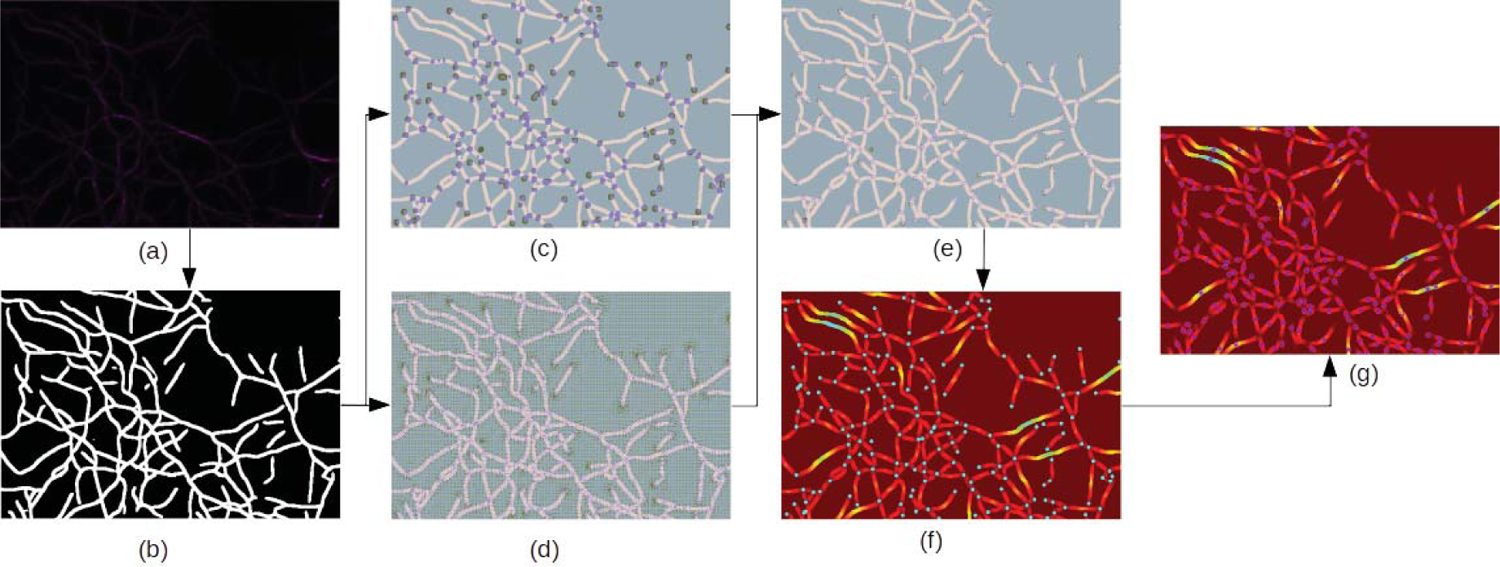
The pipeline of our proposed approach. (a) Microscopic image of actin filaments. (b) Binary segmentation. (c) Heatmaps of junctions and endpoints. (d) Offset maps of junctions and endpoints. (e) Prediction of junctions and endpoints. (f) Geodesic distance map from junctions and endpoints, which are color of cyan. (g) The local maximum value of the geodesic distance map, which is represented in blue with a pink circle. (a) to (b): We use a neural network to obtain binary segmentation. (b) to (c),(d) and (e): Our modified Resnet takes binary segmentation results as inputs and outputs offset maps and heatmaps of junctions and endpoints. Then we integrate (c) and (d) to obtain refined locations of these points. (e) to (f) and (g): We set predicted keypoints as start points and utilize a fast marching algorithm to calculate the geodesic distance map. The local peak values of the geodesic distance map can represent the half-length value of the actin filaments.

We do not use a generalized network for both binary segmentation and junction detection because we do not have labeled data for junctions. We synthesize a dataset for junction detection and train our adapted Resnet with this dataset. More details will be discussed below.

3.1. Data

3.1.1. Actin dataset

We took 10 microscopy images with a size of 1740 × 840 pixels and 17 slices in Z direction and obtained maximum intensity projection(MIP) on Z direction of these images.

3.1.2. Synthetic dataset for keypoint detection

Keypoint detection is performed on binary segmentation as we do not have junction and endpoint labels of the original images. We create 10000 images with a size of 128 × 128. As shown in Fig. 3 Each image includes a maximum of six random one-pixel width curves with a mixture of different junction types such as three-way junction and two-way junction. After we record the junction points, we randomly dilate those images with kernels of size 3 to 7. The dilated images are very similar to real binary segmented actin filament images, and we will use this synthetic dataset for training.

Fig. 3.

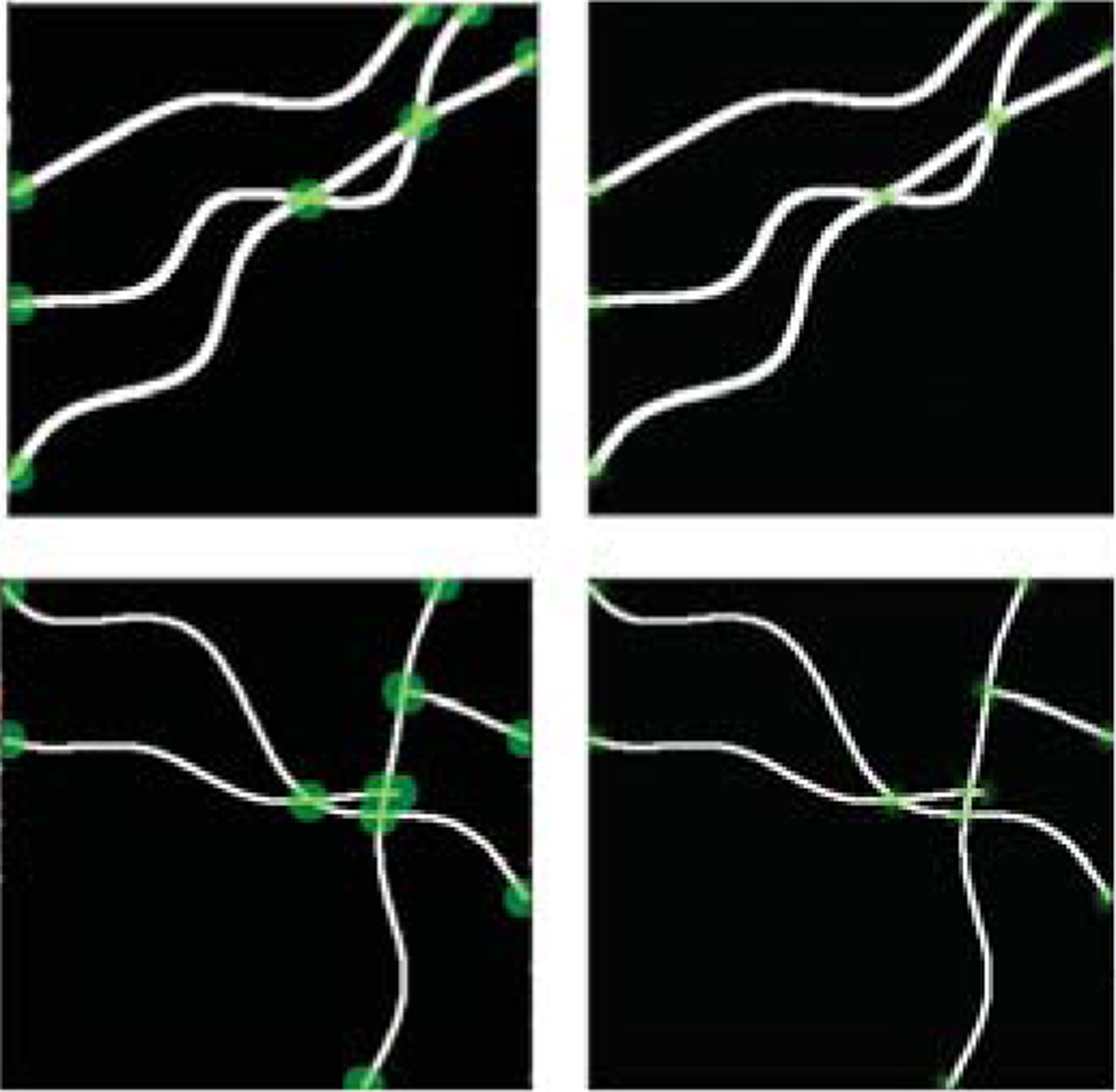
Examples of synthetic data. Left column: Disk centered around keypoints (junctions and endpoints). Right column: short-range offsets

3.2. Binary Segmentation for actin filaments

Binary segmentation is performed using the network and pre-trained weights in [11]. We use the binary segmentation results as inputs in the next step.

3.3. Keypoint detection

To detect the junctions, we use ResNet-101 as the back-bone, and we adopt the strategy in [16]. As shown in Fig. 4, We predict heatmaps for all keypoints (junctions and end-points) and offset maps (two channels per keypoint for dis-placements in the horizontal and vertical directions). Then we utilize Hough voting to aggregate heatmaps and offsets into a 2-D Hough score map. Then we locate keypoint by applying a maximum filter and locate the local maxima, which should also be higher than a threshold value. During training, we use dice-coefficient loss and L1 loss to penalize heatmaps and offsets prediction errors.

Fig. 4.

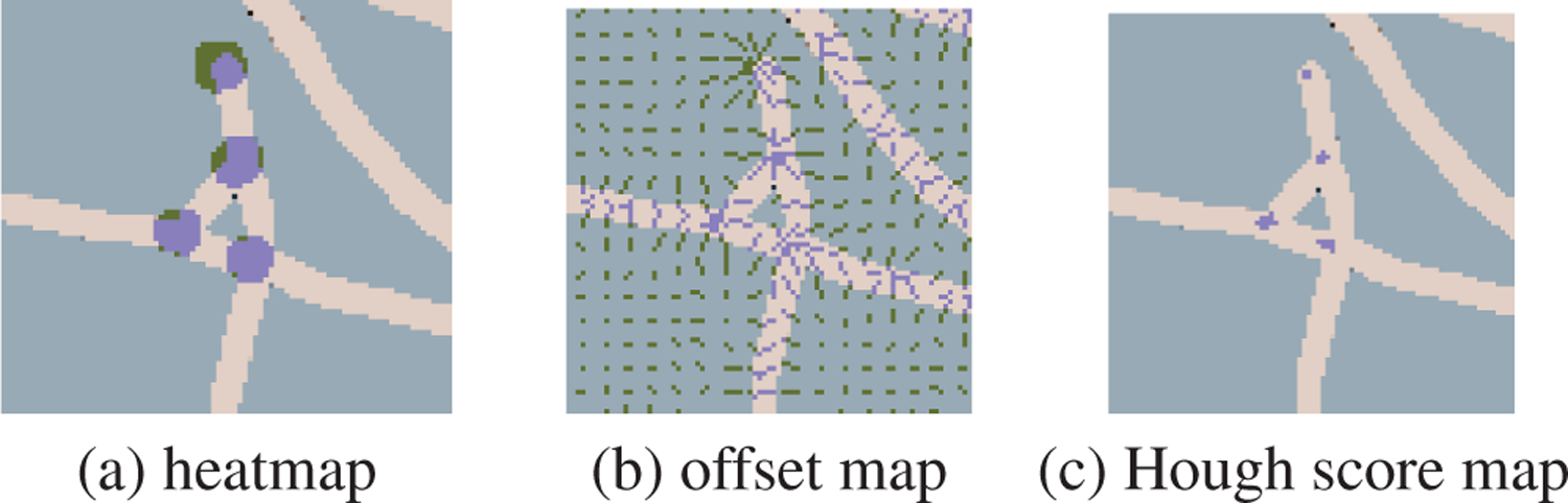
ResNet outputs (a) heatmap and (b) offsets map. Heatmap and offsets are aggregated via Hough voting into (c) Hough score map. The locations of keypoints are refined by Hough voting

3.4. Quantification analysis using a fast marching algorithm

In our work, we use a fast marching algorithm implementation [19] to compute the geodesic distance from junctions and endpoints. Since each path between junctions or endpoints represents an actin filament, we set initial contours around these keypoints. These contours grow outward with a constant speed in the local normal direction until they meet other contours or boundaries. The locations of local peak values of the distance map are the midpoints of actin filaments, and these local peak values are half of the length of filaments, as shown in Fig. 2. By doubling the peak values and counting the number of peaks, we can obtain the length and numbers of actin filaments.

4. ANALYSIS AND RESULTS

In this section, we discuss the experiments we have run, and we compare the performance of our proposed methods against other approaches.

We have run three experiments on our actin dataset: 1. SOAX [10]. 2. A method adapted from [1]. This method skeletonizes the binary segmentation first and obtains individual filaments by extracting disconnected components after disconnecting junctions. The binary segmentation we use for this method is obtained by the neural network in [11], which is the same as the one we use in the first step. 3. Our proposed approach.

Labeling individual filaments with limited resources is very difficult since there are hundreds of filaments in one image. To evaluate our approach without ground truth, we calculate the percentage difference(PD) of length, count, and average length between our approach and other methods. The formula of PD is as follows:

$$PD=\frac{A\hspace{0.17em}-\hspace{0.17em}B}{\left(A\hspace{0.17em}+\hspace{0.17em}B\right)/2}$$ (1)

As shown in table 1, the difference in total length is relatively low, which indicates that binary segmentation results are similar, and the critical difference depends on the number of filaments. As we can see from both 1 and 2, SOAX [10] obtains a much lower count on filaments, and this is because SOAX will group different contours to form a single actin filament by their geometric properties. SOAX works well with long actin filaments, but actin filaments in our microscopic images are very short and dense, and each small segment is considered an actin filament. So the results of the proposed approach and the method adapted from [1] are closer to manual count. Also, SOAX takes hours to analyze one image due to the contour-based approach, but our approach only takes seconds to run one image.

Table 1.

Quantitative comparison bewteen proposed approach and other approaches.

Model	Method adapted from [1]	SOAX [10]	Our method
Ave total length	38687.45	30990.07	47190.65
Ave filament length	20.62	46.58	29.49
Ave count per image	1876.67	665	1600
PD of total length	−0.066	−0.13	0
PD of ave length	−0.35	0.44	0
PD of count	0.14	−1.60	0

Though it requires tremendous work to manually count the filaments in each image, we only manually count the number of filaments for two images to show effectiveness of our approach, one with high PD of the count and one with low PD of the count. The result is shown in table 2.

Table 2.

Count of filaments of two images using different approaches.

Model	Image No.1	Image No.2
SOAX [10]	1147	237
Method adapted from [1]	3245	901
Our approach	2576	818
Manually count	2210	743

Fig. 5 provides a qualitative result of junction detection. Our proposed approach detects junctions more precisely, so our approach can avoid counting small false segments caused by skeletonization. The count from our proposed approach is lower than method adapted from [1], and our result is closer to ground truth value on the two selected images. More qualitative results are included in supplemental materials.

Fig. 5.

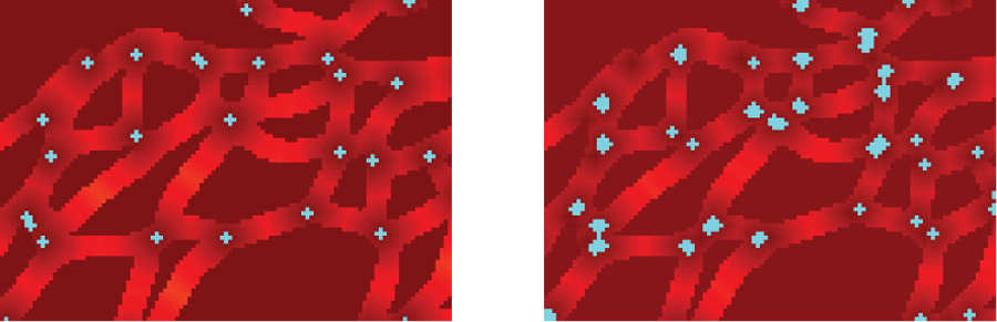
Junctions detected by our approach (Left) and junctions detected by skeletonization (Right). The thick points include more than one point. Our approach detects junctions more precisely.

5. CONCLUSION

On our dataset of actin filaments, we combine deep learning models and a fast marching algorithm to automate estimating the number and length of actin filaments in microscopic images. We have shown that our approach can successfully detect junctions and endpoints of actin filaments network, which is fundamental for estimating length using a fast marching algorithm. We prove that our approach is practical by comparing against other approaches. The total length of our approach is similar to that of other approaches, but the number of filaments predicted by us is closer to the actual number. We further prove that by showing that the count number of ours is the closet to ground truth on the two manually counted images. The main limitation of this work is unable to obtain other information such as orientation angle and curvatures, and we plan to improve our approach to quantify other features of actin filaments.