Estimation of Evapotranspiration and Energy Fluxes using a Deep-Learning based High-Resolution Emissivity Model and the Two-Source Energy Balance Model with sUAS information

Abstract

Surface temperature is necessary for the estimation of energy fluxes and evapotranspiration from satellites and airborne data sources. For example, the Two-Source Energy Balance (TSEB) model uses thermal information to quantify canopy and soil temperatures as well as their respective energy balance components. While surface (also called kinematic) temperature is desirable for energy balance analysis, obtaining this temperature is not straightforward due to a lack of spatially estimated narrowband (sensor-specific) and broadband emissivities of vegetation and soil, further complicated by spectral characteristics of the UAV thermal camera. This study presents an effort to spatially model narrowband and broadband emissivities for a microbolometer thermal camera at UAV information resolution (~0.15 m) based on Landsat and NASA HyTES information using a deep learning (DL) model. The DL model is calibrated using equivalent optical Landsat / UAV spectral information to spatially estimate narrowband emissivity values of vegetation and soil in the 7–14-nm range at UAV resolution. The resulting DL narrowband emissivity values were then used to estimate broadband emissivity based on a developed narrowband-broadband emissivity relationship using the MODIS UCSB Emissivity Library database. The narrowband and broadband emissivities were incorporated into the TSEB model to determine their impact on the estimation of instantaneous energy balance components against ground measurements. The proposed effort was applied to information collected by the Utah State University AggieAir small Unmanned Aerial Systems (sUAS) Program as part of the ARS-USDA GRAPEX Project (Grape Remote sensing Atmospheric Profile and Evapotranspiration eXperiment) over a vineyard located in Lodi, California. A comparison of resulting energy balance component estimates, with and without the inclusion of high-resolution narrowband and broadband emissivities, against eddy covariance (EC) measurements under different scenarios are presented and discussed.

1. INTRODUCTION

Thermal information provides valuable information on historical and current human and environmental activities such as vegetation and soil conditions^1–3, energy balance modeling^4–8, environmental stressor effects^9, and climate change^10–12. In agriculture, thermal information has demonstrated its importance at global, regional, farm and sub-plant scales from an array of technologies that includes thermocouples¹³, infrared radiometers^14,15, and microbolometer cameras^16–18. The infrared sensors and microbolometer cameras are technologies that can provide continuous soil, plant, and sub-plant thermal information, with applications in consumptive water use, nitrogen content, fruit/root development, crop water stress, soil moisture, and other parameters^19–22.

Thermal information from infrared technologies is affected by four major factors: radiometric calibration, atmospheric conditions (water vapor, air temperature), spectral characteristics of the instrument²³, and surface emissivity²⁴. All four factors must be addressed to adequately characterize the temperature conditions of the surface. The radiometric calibration can be addressed by using and verifying the infrared sensor’s radiometric measurements against a blackbody instrument²⁵. The atmospheric conditions can be addressed through a collection of ground temperature measurements or by using models that describe the effects of water vapor and CO₂—effects that vary with the spectral response²⁶. The other two factors are interrelated. The thermal emissivity of the surface, is related to the nature of the material and either the difference in radiation between a blackbody object and the object under study at the same temperature and infrared sensor spectral response (narrowband) or across the wavelength range of thermal response of Earth materials (3 to +15μm)²⁷. Tables and general criteria were developed to simplify assignment of emissivity values to Earth and man-made surfaces and were developed for existing thermal technology at the time of the table development (mostly satellite thermal sensors). These sensors are uniquely developed to address the four factors mentioned above, with emphasis on the selection of spectral regions that minimize atmospheric correction and allow for overall emissivity values for surface types (soil, vegetation, water). This is not the case for more recent portable or miniaturized thermal sensors, which may present significantly different emissivity values due to the broad spectral response (7 to 14μm). Still, assignment of emissivity values across agricultural or natural areas is mostly based on an initial classification of the surface (water, vegetation, and bare soil) using classification or vegetation indices (e.g., NDVI). Efforts to provide spatial emissivity estimates from satellite data exist, such as from the NASA’s ASTER Global Emissivity Dataset and ECOSTRESS programs. These estimates are being used to derive surface temperature from Landsat and ECOSTRESS²⁸. For miniaturized microbolometer sensor databases, such efforts do not exist, with only hyperspectral laboratory measurements such as the MODIS UC Santa Barbara Emissivity database, and measurements from NASA JPL Hyperspectral Thermal Emission Spectrometer (HyTES) currently available. These datasets are not well known or used by the UAV scientific community^29,30.

As shown in a previous study³¹, spatial narrowband emissivity could be estimated by a machine learning model (Random Forest) using Landsat optical bands (red, green blue, and near-infrared) vs. simultaneous emissivity values collected from the HyTES program. While the model was able to assign emissivity values to soil and vegetation, it had some limitations with surfaces such as vegetation with wet soils and service roads. The same study indicated that vegetation index–derived emissivity (NDVI) does not respond as previously reported in literature² with Landsat and HyTES datasets or a linear combination of other spectral bands. These results opened the opportunity to test complex machine learning models such as deep learning for thermal emissivity estimation. Given the range of emissivity measurements in the UC Santa Barbara dataset, broadband emissivity for different surfaces can be inferred from the database and relate it to the narrowband emissivity as derived from the deep learning (DL) model. As such, this study has two objectives: (a) test and assess the performance of a DL model in the estimation of a thermal emissivity for microbolometer cameras and (b) test the impact of spatial narrowband and broadband emissivity in the estimation of evapotranspiration with UAV information.

2. MATERIAL AND METHODS

2.1. Area of Study and UAV Sensor Description

For the current study, spatial information from NASA HyTES, Landsat, and UAV was captured in 2014, as shown in Table 1 over a Pinot Noir vineyard located near Lodi, California (38.29 N 121.12 W), in Sacramento County as part of the GRAPEX project and described in references^31,32. The UAV flight was synchronized with the Landsat satellite overpass and was operated by the AggieAir UAV research group at the Utah Water Research Laboratory at Utah State University. The study area employs a drip-irrigated system in which irrigation lines run along the base of the trellis at 30 cm agl with two emitters between each vine. The vineyard used a training system with “U” shaped trellises and canes trained upwards. The vine trellises were 3.35 m apart, and the heights to the first and second cordons were about 1.45 and 1.9 m, respectively³³.

Table 1.

Spatial products and capture times used in this study

Spatial Product	Spatial Information	Ground Resolution (m)	Capture Date and Time (PST)
NASA JPL HYTES	Hyperspectral Emissivity	6	2014-07-09 13:23
Landsat ETM+	Surface Corrected Reflectance	30	2014-07-09 10:36
AggieAir	High-Resolution Reflectance and Temperature	0.15 Reflectance 0.60 Temperature	2014-08-09 10:36

The hyperspectral emissivity information from the NASA HYTES airborne program was retrieved for this project. Details of the sensor and technology^34–37 and flown locations up to date³⁸ can be found in the references. The spatial emissivity information for the area of study covered different agricultural lands (vineyards, alfalfa) and natural environments, as presented in Fig. 1.

Fig 1.

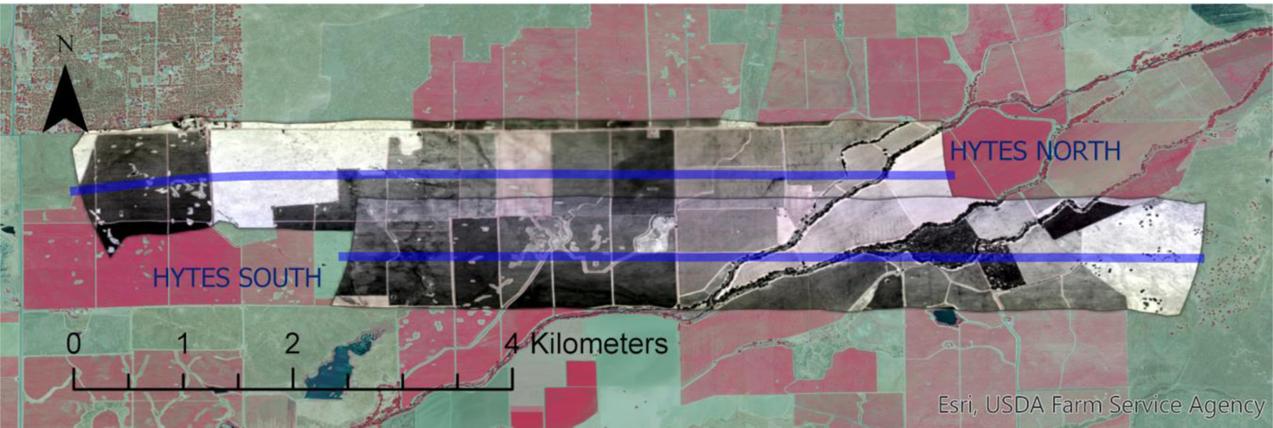
2014 NASA HYTES bands 150 (10.1 μm), 100 (9.2 μm), and 58 (8.5 μm) overpass over multiple vineyards and natural areas near Galt, CA. Two HYTES flights on the same date and time (NORTH and SOUTH, blue lines indicate flights) are used for this study.

As is evident from Table 1 and explained in a previous study³¹, a direct comparison of surface temperature between HYTES and UAV information is not possible, thus making necessary the implementation of several additional steps shown in Fig. 2 and based on the study described here³⁹.

Fig. 2.

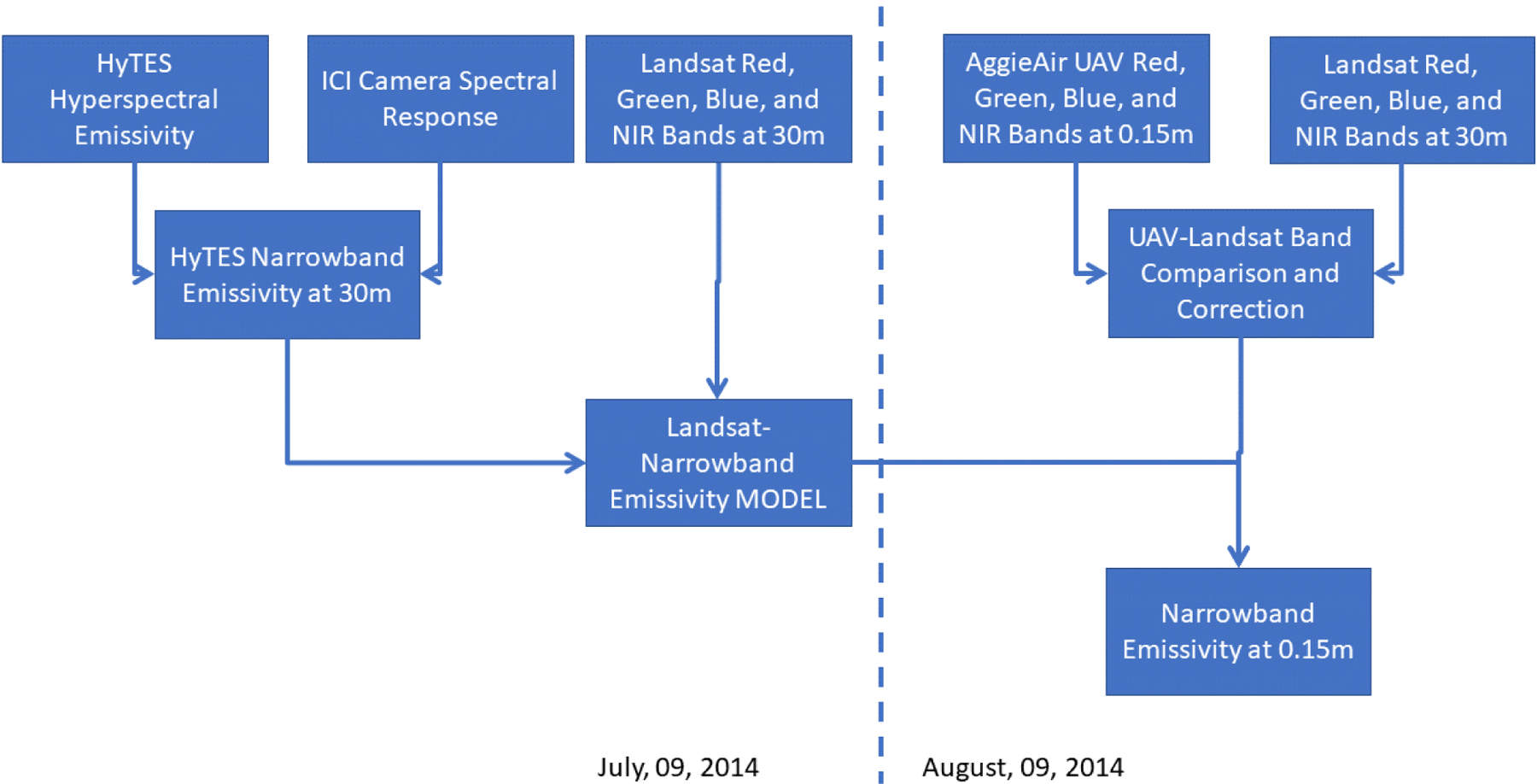
Flowchart for estimation of UAV resolution narrowband emissivity for ICI cameras as used in this study.

The different information sources are processed as described in Fig.2 for narrowband emissivity estimation. An important step is the UAV–Landsat band comparison to ensure that the reflectance values from both sensors agree, thus minimizing potential biases due to the optical sensor. A primary assumption in this analysis is the adequacy of the Landsat-Narrowband Emissivity model (developed using DL) for high-resolution imagery.

2.2. Deep Learning Emissivity Model

A DL model was calibrated using the same Landsat information as the documented Random Forest described in a previous study³¹ and Fig. 2 to estimate narrowband emissivity values. The DL model consisted of an Input Layer, Hidden Layers, and an Output Layer. The input layer consists of the Landsat bands, band ratios, and index values (i.e., four bands, six band ratios, and six Normalized Difference Indexes). The Output Layer consists of emissivity values. The hidden layers consist of a specific number of nodes that transform the input data and enable statistical interactions using activation functions (i.e., the Rectified Linear Unit function) between the inputs and outputs. A regularization method based on Lasso Regression was applied to avoid overfitting. The number of hidden layers, number of nodes per layer, number of epochs, and batch size had to be selected to find the appropriate DL model. The batch size is the number of training samples processed before the DL parameters are updated. Preliminary results showed that the optimal number of batch size was 100. Readers interested in greater detail regarding the DL model and its parameters are referred to the Keras Sequential Model page⁴⁰. The data sample consisted of 4932 observations. 70% of the data samples were used for training the model, and 30% were used for testing the model. Several DL models were built to include different parameter settings (the number of hidden layers (ranging from 1 to 4), the number of nodes per layer (ranging from 50 to 200 with increments of 50), and the number of epochs (1000 and 2000)). The goodness of statistics used for the selection of the model was the root mean square error (RMSE). The selected model is the one with the minimum RMSE corresponding to the testing phase (Table 2).

Table 2.

DL model performance for narrowband emissivity estimation based on Red, Green, Blue and Nir bands

DL Parameter Values	Inputs	Calibration scheme	Fit Statistics
Hidden Layers: 3	4 Bands: Blue, Green, Red, NIR	70 % Training	Obs: 4932
Nodes: 200	6 Ratios: Blue/Green, Blue/Red, Blue/NIR	30 % Testing	RMSE Train: 0.003
Epochs: 1000	Green/Red, Green/NIR, Red/NIR		RMSE Test: 0.004
Batch size: 100	6 Normalized Difference (ND) Indexes:
	ND_Green&Blue, ND_Red Blue, ND_NIR&Blue
	ND_Red&Green, ND_NIR&Green, ND_NIR&Red

The narrowband emissivity from the DL model and a previously trained Random Forest³¹ were numerically and visually assessed. The emissivity result with the best goodness of fit statistics was then incorporated into the radiometric temperature.

2.3. Broadband Emissivity

An additional analysis was performed based on the hyperspectral emissivity UCSB dataset (from 3 to 14μm) to approximate the broadband emissivity estimates at the UAV pixel scale, using the narrowband emissivity estimation. The broadband emissivity is necessary to estimate the Outgoing Longwave Radiation, as part of the Net Radiation, once the surface (kinematic) temperature is available⁴¹. Given the closeness of the spectral range of the narrowband to the broadband emissivities, the narrowband to broadband model was developed first by estimating the narrowband emissivity by the ratio of the convolved sum-product UCSB emissivity, microbolometer spectral response and the Planck equation at a temperature of 300K, and the convolved sum-product of the microbolometer spectral response and the Planck equation. The broadband emissivity was calculated as the sum-product of hyperspectral emissivity and the Planck equation divided by the sum of the Planck equation for the 3 to 14 μm⁴². Additional details are presented in the following section.

2.4. Two-Source Surface Energy Balance model

To test the impact of sensor-specific and broadband emissivity in this study, the Two-Source Energy Balance (TSEB) model with the Canopy and Soil (also called Dual) Temperature estimation as described by Nieto et al.⁴¹ is used. The Dual Temperature approach is shown in Fig 3. In this figure, the estimation/separation of the canopy and soil temperature within a spatial domain grid is achieved by the linear behavior of NDVI (or any other vegetation index) with temperature and defining soil or canopy average temperature conditions by thresholds that identify these two vegetation conditions. For example, bare soil threshold is NDVI below or equal to 0.3, and fully developed vegetation threshold is NDVI equal to or higher than 0.75).

Fig. 3.

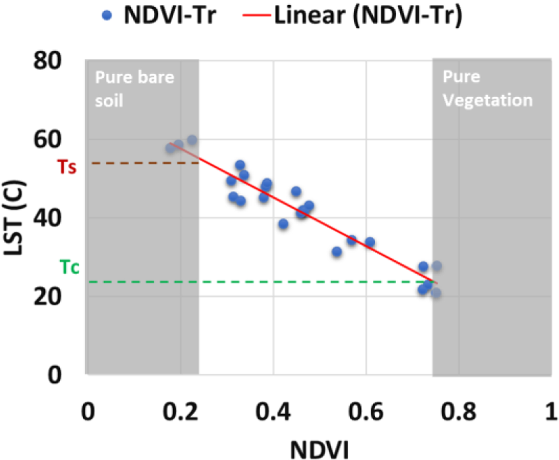
Canopy (Tc) and Soil (Ts) Temperature estimation over spatial domain grid based on a linear relationship between NDVI and Land Surface Temperature (LST).

The TSEB model can use radiometric or kinematic temperature to infer (radiometric or kinematic, respectively) canopy and soil temperature, which in turn are used to estimate energy balance components for each of them. Typically, the radiometric temperature is used due to the lack of spatially estimated emissivity. Assuming no atmospheric correction is needed, the estimation of kinematic temperature from radiometric temperature is:

$$Ts={(1/\epsilon )}^{0.25}Tr$$ (1)

where Ts is the kinematic temperature, ε is the narrowband emissivity, and Tr is the radiometric temperature, as provided by the infrared thermal sensor. Internally, the TSEB model does not assign a narrowband emissivity to vegetation and soil conditions. Also, internally, the TSEB model estimates the Net Radiation components, which requires solving the absorption and reflection of short-wave radiation, as well as the outgoing and incoming long-wave radiations, expressed as follows:

$$Rn=(1-\alpha )Rs-L\uparrow +L\downarrow$$ (2)

where Rn is the net radiation (W m−2), Rs is the solar radiation (W m−2), α is the soil surface albedo (α = 0–1), L↑ is the outgoing long-wave radiation (W m−2) from the Earth’s surface, and L↓ is the long-wave incoming radiation (W m−2) from the sky. The long-wave radiation uses the broadband emissivity and the kinematic temperature:

$$L\uparrow =\epsilon b\left(\sigma T{s}^4\right)$$ (3)

where εb is the broadband emissivity, σ is the Stefan-Boltzmann coefficient, and Ts is the kinematic temperature. A traditional broadband emissivity value of 0.98 for vegetation and 0.95 for soil is assigned as implemented within the TSEB model.

The incoming long-wave radiation values are obtained from eddy covariance (EC) instrumentation for clear skies, or it can be calculated as follow:

$$L\downarrow =\epsilon a\left(\sigma T{a}^4\right)$$ (4)

where εa is the air emissivity, and Ta is the air temperature at 2 m elevation from the ground. Figure 4 describes in detail the TSEB model process as well as the use of radiometric temperature and incoming and outgoing longwave radiation to solve the surface energy balance model.

Fig. 4.

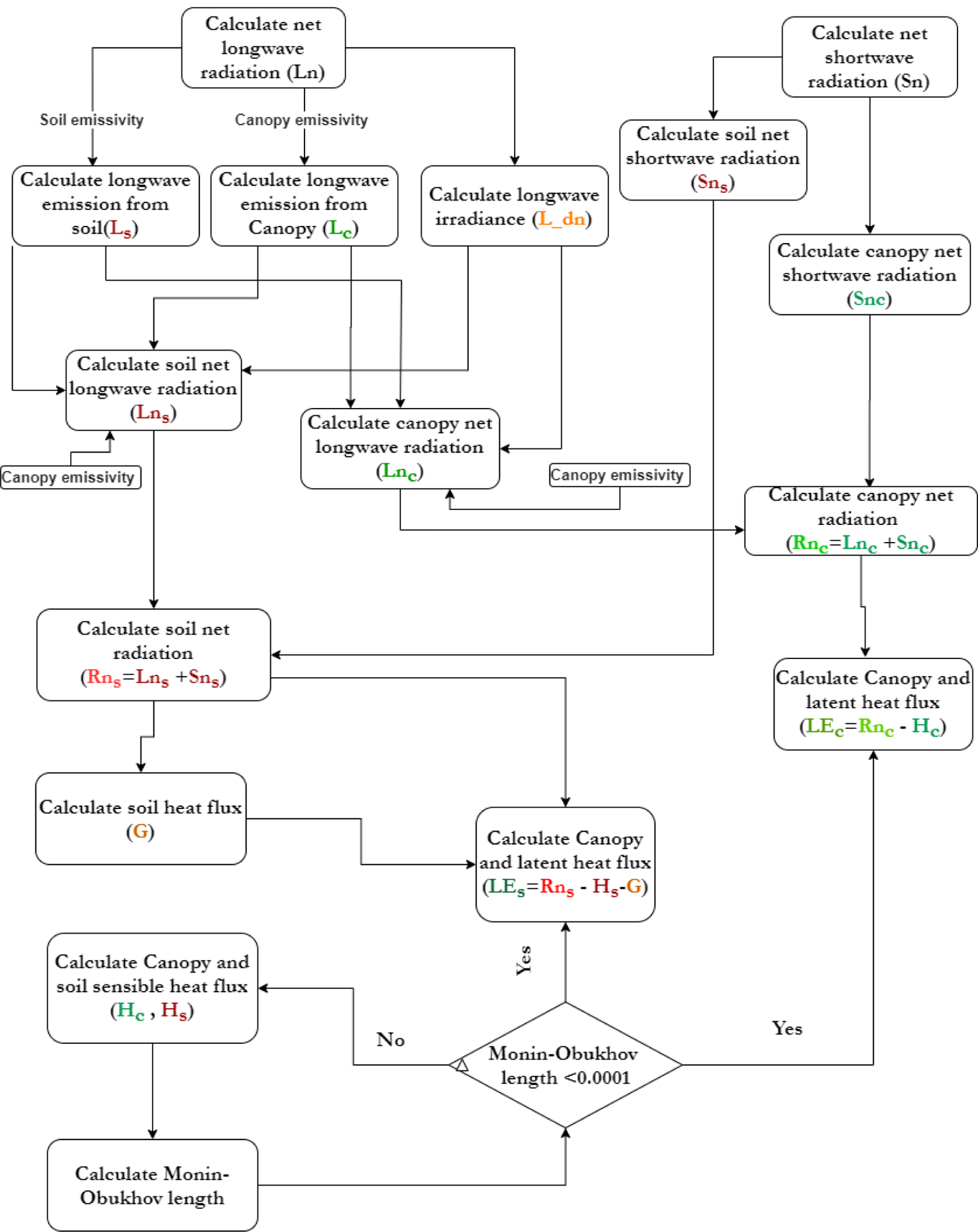
Example of the TSEB Dual Temperature data processing. Note the broadband emissivity parameters used in the model for characterization of the soil and canopy energy balance components.

As result of the TSEB model run, the instantaneous estimates of the four Energy Balance components are produced. These components are Rn: Net Radiation, G: Ground Heat Flux, H: Sensible Heat Flux, and LE: Latent Heat Flux, the last of which is the equivalent of evapotranspiration, in energy units (W/m2).

3. RESULTS

3.1. Narrowband Emissivity Model

Figure 5 shows the overall performance of the DL model for the estimation of narrowband emissivity using Landsat reflectance and NASA HyTES information. The scatter plot pattern indicates that, while the DL model results approximate the emissivity values, there are still conditions where the estimated emissivity does not relate to HyTES-derived emissivity. This limited relationship might be due to a potential issue where two or more inputs of the model are linearly related (multicollinearity) or the reduced relationship between used inputs and emissivity. This potential issue could lead to the wrong identification of relevant inputs and can affect the results. However, these are not definite conclusions, as they might not be sufficiently well supported. A more detailed analysis regarding strategies to improve the DL model performance will be carried out for future research. Still, Figs. 5 to 7 shows a better statistical performance of the DL model vs. the previously reported Random Forest model.

Figure 5.

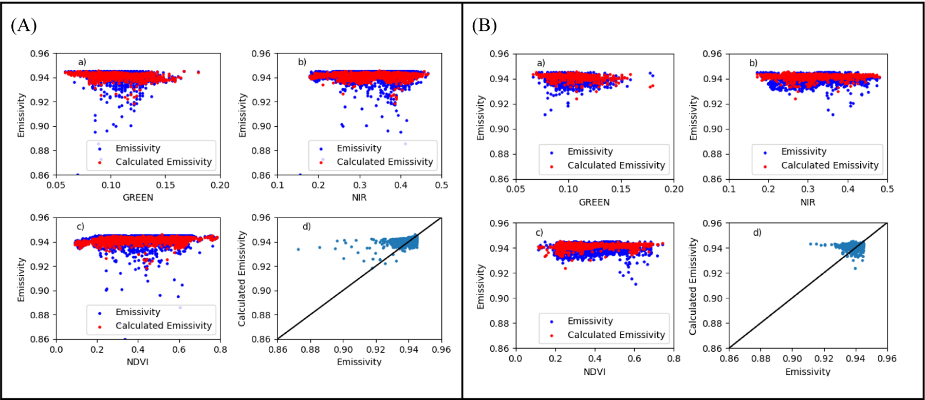
DL narrowband emissivity model performance (A) Training Phase, (B) Test Phase

Figure 7,

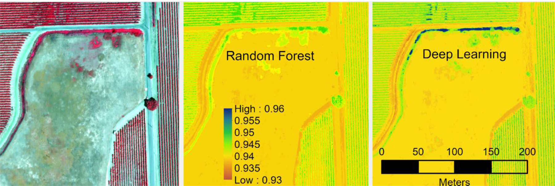
Close up of the Visual (left) and Narrowband Emissivity results from Random Forest (center) and DL (right) models

A visual comparison at UAV resolution (0.15m/pixel) between the DL and previously reported Random Forest models is presented in Figure 6 and 7.

Figure 6.

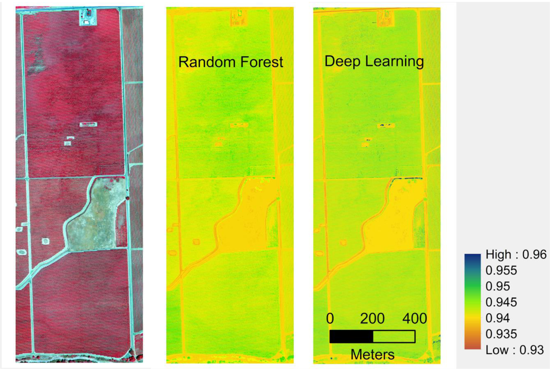
Visual (left) and Narrowband Emissivity results from Random Forest (center) and DL (right) models

Visual assessment of the produced emissivity at UAV optical resolution (0.15m) in Fig. 6 indicates that obtained emissivity values by the DL model better represents the soil, vegetation, and water conditions than the results obtained by the Random Forest. Figure 7 clearly illustrates this statement. A shallow wet earth canal displayed in the figure, fully covered by vegetation, is assigned emissivity values closer to 0.95 by the Random Forest model but higher than 0.96 by the DL model. The higher emissivity values go along with the expected soil moisture, water, and healthy vegetation emissivity. For soil emissivity, assigned values of 0.93 and 0.94 are similar in both emissivity models. Grapevine plant emissivity is higher in the DL model (0.95 and higher), while emissivity values for the Random Forest model are lower than 0.95. Based on these results, the DL emissivity model results will be incorporated into the TSEB model. Still, the DL model has some limitations on specific surfaces and locations (emissivity values under shaded conditions in the image were negative). In those cases, the DL emissivity results were replaced with the Random Forest results.

3.2. Broadband Emissivity

To estimate the broadband emissivity, water, soil, and vegetation emissivity samples from the UCSB emissivity archive, were processed as described in the methodology, along with a narrowband emissivity estimation for the ICI microbolometer UAV camera. The narrowband and broadband emissivity relationship and resulting linear equation are presented in Fig. 8.

Fig. 8.

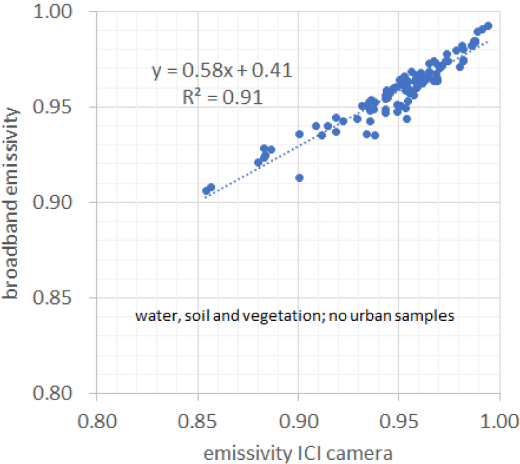
Broadband vs. ICI camera (narrowband) emissivity relationship based on the UCSB water, soil, and vegetation emissivity archive.

The found relationship of broadband to narrowband emissivity approximates a linear relationship, due to the broad spectral response of the ICI camera (7 to 14μm)²⁵. It is expected that other microbolometer sensors and infrared radiometers have a similar relationship due to their similar broad spectral response. Still, improvements to this equation can be made by separating the information in Fig. 8 by the type of surface (water, soil, vegetation) and developing separated relationships. For the purposes of this study, the presented equation is used then to estimate broadband emissivity from the DL emissivity results spatially.

3.3. Impact of Emissivity in the TSEB Model

The scheme detailed below was implemented to assess the impact of incorporating the spatial narrowband and broadband emissivities in the estimation of energy fluxes (net radiation, ground heat flux, and sensible and latent heat flux) in the TSEB model.

Ground Truth information

• EC measured fluxes (Ground Truth information)

Incorporation of emissivity schemes:

• Default TSEB narrowband and broadband emissivity values (no narrowband emissivity and 0.98 and 0.95, respectively, for vegetation and soil for broadband emissivity) (Emis Fixed)

• Incorporation of narrowband emissivity in the radiometric temperature using only Equation (1) (DL emis)

• Incorporation of narrowband and broadband emissivity in the TSEB model (Equations 1 and 3) (DL and Broadband emis)

The incorporation of emissivity schemes was evaluated under the following four scenarios:

• Using UAV radiometric temperature and using EC Incoming Long-wave Radiation (L↓) measured by Eddy Covariance (Tr Original and Measured L↓).

• Using UAV radiometric temperature and using Incoming Long-wave Radiation equation 4 (Tr Original and Calculated L↓).

• Using UAV radiometric temperature with atmospheric correction as described by Torres²⁵ and using EC Downwelling Radiation measured by the EC instruments (Tr Corrected and Measured L↓).

• Using UAV radiometric temperature with atmospheric correction as described by Torres²⁵ and using Incoming Longwave Radiation equation 4 (Tr Corrected and Calculated L↓).

These scenarios respond to the potential cases of radiometric temperature measurements and the Incoming Longwave Radiation information availability. These four incorporations of emissivity and four scenarios were evaluated under two EC instruments (North and South), over which the proposed analysis was performed. The location of the EC towers (red dots) and their footprint area (yellow area) are presented in Figure 9.

Figure 9.

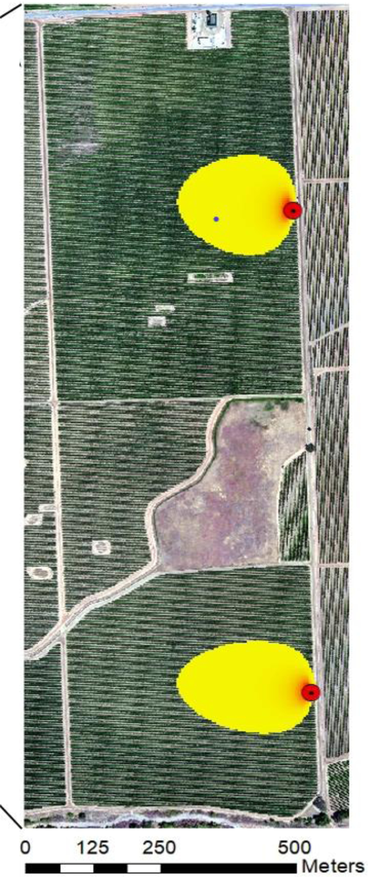
North (top) and South (bottom) EC towers located in the area of study.

The results of incorporating the emissivity values (narrowband and broadband) under different proposed scenarios in the TSEB model is presented in Fig 10.

Fig 10.

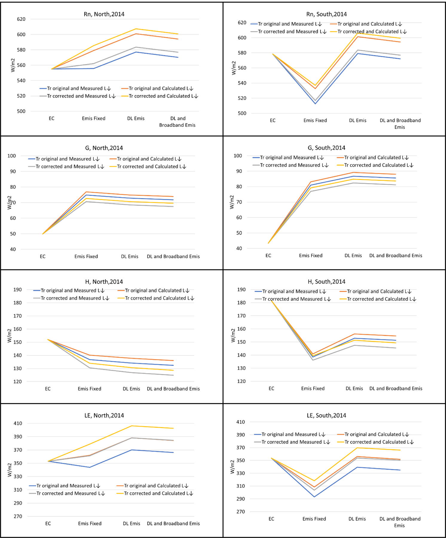
Energy Flux comparisons between EC) measurements (NORTH, left column, SOUTH, right column) and proposed scenarios using different radiometric temperature information.

The detail in Fig. 10 provides the necessary information to assess the defined schemes and scenarios for incorporation of emissivity (narrowband and broadband). Overall, inclusion of emissivity causes a small improvement in the estimated energy balance components when compared against the EC values. The default emissivity results (Emis Fixed) tend to be slightly better or equivalent to the eddy covariance energy balance components, although the incorporation of spatial emissivities (DL Emis and DL and Broadband Emis) significantly improve the performance of energy balance components for the SOUTH EC location. The improvement may occur because the emissivity values are likely adjusting the temperature values to the different vegetation conditions in the SOUTH location. Regarding the four evaluated scenarios, no preferable scenario emerged; although, for the Calculated L↓(incoming radiation) scenario, energy balance components performed similarly to the Measured L↓. The similarity between Calculated and Measured incoming radiation is an indication that, for a location with no EC instrumentation, the incoming radiation will be adequately calculated. With regards to atmospherically Corrected vs. Original UAV temperature information, no clear difference was identified between the energy balance results under the different schemes and scenarios. This limited difference implies that, despite the effect from the atmosphere on the thermal information, the TSEB model is not sensitive to it, and estimated energy balance components under the emissivity information and the proposed scenarios are similar.

A similar discussion can be done for each energy balance component. For Net Radiation (Rn), the scenario using NORTH and SOUTH EC locations, including emissivity (LD emis and DL and Broadband emis), and using Measured L↓ performs similar or better than Emis fixed. The Ground Heat Flux (G) value, which is internally estimated in TSEB, is overestimated for all emissivity schemes and scenarios. No preferable scheme nor scenario emerged, given the same estimate G value. For Sensible Heat Flux (H), the emissivity schemes and four scenarios provide equal or better estimates than the default TSEB (Emis fixed), although for all schemes and scenarios, H is underestimated, with no preferable scheme or scenario. Finally, for Latent Heat Flux (LE), the schemes and scenarios performed similarly or better than the default TSEB (Emis fixed). Differences between schemes and scenarios are minimal, with none prefered over any other.

These results, while performed over a single agricultural site and data, allows for the following overall conclusions. Spatial emissivity estimation (narrowband and broadband) does improve the energy balance model estimates, although in a small manner. Thus, whenever the availability of emissivity information from models like the proposed DL model used in this study or another is possible, then these emissivity values should be included in the analysis. The inclusion of only narrowband (DL emis) vs. both narrowband and broadband emissivities (DL and Broadband Emis) in the TSEB model in this study seems to indicate that the performance of these two schemes is similar, but using both by making use of relationships between the ~7 to ~14μm narrowband to broadband emissivity is still preferable, as derived in this study. Another point for consideration is the atmospheric correction of thermal images, which does not seem to influence the estimation of energy balance in the TSEB model, making it suitable to the range of optical and thermal instrumentation available for UAVs. The use of calculated L↓ performed well in this analysis, encouraging the use of the TSEB model with agricultural weather station information. One caveat of these findings is that these may not be extendable to other surface energy balance models that make use of temperature information due to the uniqueness of the dual temperature approach. Thus it is advisable to perform a similar effort to determine their sensitivity to emissivity for the sensor and broadband estimates.

4. CONCLUSIONS

Estimation of surface temperature enhances vegetation and soil condition monitoring efforts in agriculture. To achieve surface temperature, estimation of emissivity is necessary. For UAVs temperature sensors, emissivity estimates can differ from traditionally emissivity values due to the waveband. In this study, an effort to improve the spatial estimation of thermal emissivity for UAV technologies using a DL algorithm is evaluated as along with its impact on the temperature information used to estimate surface energy balance. For this work, Landsat optical information, NASA HyTES emissivity, and UAV data were used to spatially estimate narrowband and broadband emissivities and test under three schemes (fixed emissivity, narrowband emissivity, and narrowband and broadband emissivities) and four scenarios which contemplate the combination of UAV radiometric and atmospherically corrected temperature as also considering incoming radiation (measured and calculated). The energy balance model considered was the Two-Source Energy Balance model. Compared to the previously published work³¹, which used a Random Forest algorithm for estimation of emissivity, the DL model provides an improvement, especially in locations with confounding factors (water, soil, healthy vegetation). Additional data sets and locations can improve these initial results from this DL implementation. In terms of improvements to the estimation of surface energy balance and evapotranspiration, the TSEB model was shown to be insensitive to the changes in temperature and radiation that the schemes and scenarios provided and saw a small improvement in energy flux estimation by the inclusion of emissivity, thus its use is recommended whenever this information is available. Nevertheless, the documented insensitivity of the TSEB model to changes in temperature and radiation allows for its use with other UAV optical and thermal sensors, as currently available in the UAV sensor market.

REFERENCES

- [1].Berni JAJ, Zarco-Tejada PJ, Suarez L and Fereres E, “Thermal and Narrowband Multispectral Remote Sensing for Vegetation Monitoring From an Unmanned Aerial Vehicle,” IEEE Trans. Geosci. Remote Sens 47(3), 722–738 (2009). [Google Scholar]
- [2].Van de Griend AA AND OWE M, “On the relationship between thermal emissivity and the normalized difference vegetation index for natural surfaces,” Int. J. Remote Sens 14(6), 1119–1131 (1993). [Google Scholar]
- [3].Ochsner TE, Horton R and Ren T, “A New Perspective on Soil Thermal Properties,” Soil Science Society of America Journal 65(6), 1641–1647 (2001). [Google Scholar]
- [4].Carlson TN, Dodd JK, Benjamin SG and Cooper JN, “Satellite Estimation of the Surface Energy Balance, Moisture Availability and Thermal Inertia,” J. Appl. Meteorol 20(1), 67–87 (1981). [Google Scholar]
- [5].Bastiaanssen WGM, Menenti M, Feddes RA and Holtslag AAM, “A remote sensing surface energy balance algorithm for land (SEBAL). 1. Formulation,” J. Hydrol 212–213(1–4), 198–212 (1998). [Google Scholar]
- [6].Ling F and Zhang T, “A numerical model for surface energy balance and thermal regime of the active layer and permafrost containing unfrozen water,” Cold Regions Science and Technology 38(1), 1–15 (2004). [Google Scholar]
- [7].Jacob F, Olioso A, Gu XF, Su Z and Seguin B, “Mapping surface fluxes using airborne visible, near infrared, thermal infrared remote sensing data and a spatialized surface energy balance model,” Agronomie 22(6), 669–680 (2002). [Google Scholar]
- [8].Anderson MC, Allen RG, Morse A and Kustas WP, “Use of Landsat thermal imagery in monitoring evapotranspiration and managing water resources,” Remote Sens. Environ 122, 50–65 (2012/July). [Google Scholar]
- [9].Voogt JA and Oke TR, “Thermal remote sensing of urban climates,” Remote Sensing of Environment 86(3), 370–384 (2003). [Google Scholar]
- [10].Johannessen OM, Bengtsson L, Miles MW, Kuzmina SI, Semenov VA, Alekseev GV, Nagurnyi AP, Zakharov VF, Bobylev LP, Pettersson LH, Hasselmann K and Cattle HP, “Arctic climate change: observed and modelled temperature and sea-ice variability,” Tellus A: Dynamic Meteorology and Oceanography 56(5), 559–560 (2004). [Google Scholar]
- [11].Guilderson TP, Fairbanks RG and Rubenstone JL, “Tropical temperature variations since 20,000 years ago: modulating interhemispheric climate change,” Science 263(5147), 663–665 (1994). [DOI] [PubMed] [Google Scholar]
- [12].van Vliet MTH, Franssen WHP, Yearsley JR, Ludwig F, Haddeland I, Lettenmaier DP and Kabat P, “Global river discharge and water temperature under climate change,” Global Environmental Change 23(2), 450–464 (2013). [Google Scholar]
- [13].Ramos L, Villar D and Cabezas OA, “Water stress index (CWSI) of rice ir 71706 via calibrated canopy thermography in the molina, peru,” Agu Fall Meeting 2019, Agu (2019). [Google Scholar]
- [14].Blonquist JM Jr., Norman JM and Bugbee B, “Automated measurement of canopy stomatal conductance based on infrared temperature,” Agric. For. Meteorol 149(12), 2183–2197 (2009). [Google Scholar]
- [15].Lebourgeois V, Chopart J-L, Bégué A and Le Mézo L, “Towards using a thermal infrared index combined with water balance modelling to monitor sugarcane irrigation in a tropical environment,” Agricultural Water Management 97(1), 75–82 (2010). [Google Scholar]
- [16].Wang S, Garcia M, Bauer-Gottwein P, Jakobsen J, Zarco-Tejada PJ, Bandini F, Paz VS and Ibrom A, “High spatial resolution monitoring land surface energy, water and co2 fluxes from an unmanned aerial system,” Remote Sens. Environ 229, 14–31 (2019). [Google Scholar]
- [17].Malbéteau Y, Parkes S, Aragon B, Rosas J and Mccabe M, “Capturing the Diurnal Cycle of Land Surface Temperature Using an Unmanned Aerial Vehicle,” Remote Sensing 10(9), 1407 (2018). [Google Scholar]
- [18].Hassan-Esfahani L, Torres-Rua A, Jensen A and Mckee M, “Spatial Root Zone Soil Water Content Estimation in Agricultural Lands Using Bayesian-Based Artificial Neural Networks and High-Resolution Visual, Nir, and Thermal Imagery,” Irrigation and Drainage 66(2), 273–288 (2017). [Google Scholar]
- [19].Weng Q, “Thermal infrared remote sensing for urban climate and environmental studies: methods, applications, and trends,” ISPRS Journal of Photogrammetry and Remote Sensing 64(4), 335–344 (2009). [Google Scholar]
- [20].Quattrochi DA and Luvall JC, “Thermal Infrared Remote Sensing For Analysis of Landscape Ecological Processes: Current Insights and Trends,” Scale Issues In Remote Sensing, 34–60 (2014). [Google Scholar]
- [21].Khanal S, Fulton J and Shearer S, “An overview of current and potential applications of thermal remote sensing in precision agriculture,” Computers and Electronics in Agriculture 139, 22–32 (2017). [Google Scholar]
- [22].Wang L and Qu JJ, “Satellite remote sensing applications for surface soil moisture monitoring: a review,” Frontiers of Earth Science in China 3(2), 237–247 (2009). [Google Scholar]
- [23].Zhirong LIZR and Mcdonnell MJ, “Atmospheric correction of thermal infrared images,” International Journal of Remote Sensing 9(1), 107–121 (1988). [Google Scholar]
- [24].Hulley GC, Hook SJ, Abbott E, Malakar N, Islam T and Abrams M, “The Aster Global Emissivity Dataset (ASTER GED): Mapping Earth’s emissivity at 100 meter spatial scale: aster Emissivity Dataset,” Geophys. Res. Lett 42(19), 7966–7976 (2015). [Google Scholar]
- [25].Torres-Rua A, “Vicarious Calibration of sUAS Microbolometer Temperature Imagery for Estimation of Radiometric Land Surface Temperature,” Sensors 17(7) (2017). [DOI] [PMC free article] [PubMed] [Google Scholar]
- [26].Berk A, Bernstein LS and Robertson DC, [Modtran: A Moderate Resolution Model for LOWTRAN 7] (1989). [Google Scholar]
- [27].Idaho, U. of., “Metric Mapping Evapotranspirationat High Resolution using Internalized Calibration: Applications Manual for Landsat Satellite Imagery.”
- [28].Johnson WR, Hook SJ, Schmitigal WP, Gullioud R, Logan TL and Lum KT, “ECOSTRESS End-To-End Radiometric Validation,” 2019 IEEE Aerospace Conference (2019). [Google Scholar]
- [29].Wan Z, Ng D and Dozier J, “Spectral Emissivity measurements of land-surface materials and related radiative transfer simulations,” Adv. Space Res 14(3), 91–94 (1994). [Google Scholar]
- [30].Wan Z, “MODIS (Moderate Resolution Imaging Spectrometer) UCSB Emissivity Library,” USCB Emissivity Library, 10 November 1999, <https://www.icess.ucsb.edu/modis/emis/html/em.html> (16 March 2020). [Google Scholar]
- [31].Torres-Rua A, Aboutalebi M, Wright T, Nassar A, Guillevic P, Hipps L, Gao F, Jim K, Alsina MM, Coopmans C, Mckee M and Kustas W, “Estimation of surface thermal emissivity in a vineyard for uav microbolometer thermal cameras using nasa hytes hyperspectral thermal, and landsat and aggieair optical data,” Autonomous Air and Ground Sensing Systems For Agricultural Optimization and Phenotyping Iv 11008, 1100802, International Society For Optics and Photonics (2019). [DOI] [PMC free article] [PubMed] [Google Scholar]
- [32].Torres-Rua A, Nieto H, Parry C, Elarab M, Collatz W, Coopmans C, Mckee L, Mckee M and Kustas W, “Inter-comparison of thermal measurements using ground-based sensors, UAV thermal cameras, and eddy covariance radiometers,” Autonomous Air and Ground Sensing Systems for Agricultural Optimization and Phenotyping Iii 10664, 106640e, International Society for Optics and Photonics (2018). [DOI] [PMC free article] [PubMed] [Google Scholar]
- [33].Kustas William P, Knipper Kyle, Anderson Martha, Nieto Hector, Torres-Rua Alfonso F, Mckee Mac, Prueger John H, Alfieri Joseph G, Hain Christopher, Mckee Lynn, Yang Yun, Gao Feng, Wilson Tiffany G, Hipps Lawrence, Alsina Maria Mar, Dokoozlian Nick, Sanchez Luis., “Grapex: A Project Integrating Ground, Aerial and Satellite Observations for Improved Water Management of Vineyards” (10–14 December 2018). [Google Scholar]
- [34].Hook SJ, Johnson WR and Abrams MJ, “Nasa’s Hyperspectral Thermal Emission Spectrometer (HyTES),” [Thermal Infrared Remote Sensing: Sensors, Methods, Applications], Kuenzer C and Dech S, Eds., Springer Netherlands, Dordrecht, 93–115 (2013). [Google Scholar]
- [35].Johnson WR, Hook SJ, Mouroulis P, Wilson DW, Gunapala SD, Realmuto V, Lamborn A, Paine C, Mumolo JM and Eng BT, “Hytes: Thermal imaging spectrometer development,” 2011 Aerospace Conference, 1–8 (2011). [Google Scholar]
- [36].Gillespie A, Rokugawa S, Matsunaga T, Cothern JS, Hook S and Kahle AB, “A temperature and emissivity separation algorithm for Advanced Spaceborne Thermal Emission and Reflection Radiometer (ASTER) images,” IEEE Transactions on Geoscience and Remote Sensing 36(4), 1113–1126 (1998). [Google Scholar]
- [37].Seemann SW, Borbas EE, Knuteson RO, Stephenson GR and Huang H-L, “Development of a Global Infrared Land Surface Emissivity Database for Application To Clear Sky Sounding Retrievals from Multispectral Satellite Radiance Measurements,” Journal of Applied Meteorology and Climatology 47(1), 108–123 (2008). [Google Scholar]
- [38].“Welcome To Hyperspectral Thermal Emission Spectrometer website — Hyperspectual Thermal Emission Spectrometer.”, <https://hytes.jpl.nasa.gov/> (4 March 2019).
- [39].Aboutalebi Mahyar, Alfonso Torres-Rua Mac Mckee, Nieto Hector, Kustas William, Prueger John, Mckee Lynn, Alfieri Joseph, Hipps Lawrence, Coopmans Calvin., “Assessment of Landsat Harmonized sUAS Reflectance Products Using Point Spread Function (Psf) On Vegetation Indices (VIs) and Evapotranspiration (ET) Using the Two-Source Energy Balance (TSEB) Model” (2018). [Google Scholar]
- [40].“Guide to the Sequential model - Keras Documentation.”, <https://keras.io/getting-started/sequential-model-guide/> (1 April 2020).
- [41].Nieto Solana H, Kustas WP, Torres-Rua AF, Elarab M, Song L, Alfieri JG, Prueger JH, Mckee L, Anderson MC, Alsina MM, Jensen A and Mckee M, “Advances in the Two Source Energy Balance (TSEB) model using very high resolution remote sensing data in vineyards” (2015). [Google Scholar]
- [42].Hulley GC, Ghent D, Göttsche FM, Guillevic PC, Mildrexler DJ and Coll C, “3 - Land Surface Temperature,” [Taking the Temperature of the Earth], Hulley GC and Ghent D, Eds., Elsevier, 57–127 (2019). [Google Scholar]