The Ionospheric Connection Explorer Mission: Mission Goals and Design

Abstract

The Ionospheric Connection Explorer, or ICON, is a new NASA Explorer mission that will explore the boundary between Earth and space to understand the physical connection between our world and our space environment. This connection is made in the ionosphere, which has long been known to exhibit variability associated with the sun and solar wind. However, it has been recognized in the 21st century that equally significant changes in ionospheric conditions are apparently associated with energy and momentum propagating upward from our own atmosphere. ICON’s goal is to weigh the competing impacts of these two drivers as they influence our space environment. Here we describe the specific science objectives that address this goal, as well as the means by which they will be achieved. The instruments selected, the overall performance requirements of the science payload and the operational requirements are also described. ICON’s development began in 2013 and the mission is on track for launch in 2017. ICON is developed and managed by the Space Sciences Laboratory at the University of California, Berkeley, with key contributions from several partner institutions.

1. Introduction

The way in which planetary atmospheres interact with their space environments has emerged as a top science priority for NASA [Jakosky et al., 2015; Bougher et al., 2015]. New focus and interest in this topic in the terrestrial environment has originated in a number of recent and surprising discoveries that highlight the apparent influence of the troposphere and stratosphere on conditions well above the boundary of space (~100 km altitude at Earth), extending to the peak in the ionosphere (~ 300 km) [cf. Sagawa et al., 2005; Immel et al., 2006, 2009; England et al., 2006, 2008, 2009; Hagan et al., 2007; Goncharenko et al., 2010]. Global-scale imaging of the ionosphere afforded by a number of NASA and DoD missions has provided one of the keys to realizing this apparent connection. [Mende et al., 2000; Christensen et al., 2003] Though the solar and solar wind inputs to this region (and geospace as a whole) are now well quantified, the potential drivers of ionospheric variability originating from the troposphere and stratosphere are not. ICON is a single spacecraft mission that measures and analyzes these drivers, combining for the first time remote optical and in situ plasma measurements of observables that are tied together by Earth’s magnetic field. In this way, ICON simultaneously retrieves all of the properties of the system that both influence and result from the dynamical and chemical coupling of the atmosphere and ionosphere. With this approach, ICON will give us the ability to explain how energy and momentum from the lower atmosphere propagate into the space environment, how they are connected to the large day-today ionospheric variability, and how these drivers set the stage for the extreme conditions of solar-driven magnetic storms.

The roots of ICON’s science mission go back to many sources. One of the most broadly important theoretical efforts of the space age was by Hines [1960]. In this work was the first theoretical description of gravitationally bound atmospheric waves that could exist in Earth’s atmosphere and extend naturally from the surface to heights well above 100 km, depending upon their wave characteristics and background conditions. It had also become clear over time that the large-scale motion of the upper atmosphere bore many similarities to the natural tidal oscillations that had long been observed in the troposphere, mainly through barometric pressure observations. This realization came over time as the capability for deriving motion of the neutral gas in the ionosphere was developed using ground-based magnetometer observations combined later with better measurements and knowledge of the daytime E-region of the ionosphere [Chapman, 1919; Fejer, 1953; Vestine, 1954; Kato 1956, 1966; Hines, 1963, 1966; Chapman and Lindzen, 1970] However, the observed properties of tides in the upper atmosphere and the overall variation in the near-Earth space environment with season, solar cycle, and from year to year [cf., Mayr et al., 1976; Hernandez and Roble, 1976; Woodman et al., 1977; Park et al., 1978] presented a number of challenges to theoretical treatments. Extensive theoretical development [cf., Volland and Mayr, 1977, Schunk and Nagy, 1978; Torr et al., 1979,], solar observations [Hall and Hinteregger, 1970] and laboratory work [see the many reports by T. Slanger including Slanger and Black, 1974, 1976] paved the way for computational approaches in the 1980s [Rishbeth et al., 1987; Roble et al., 1988] that in turn spurred a drive for validation; specifically: height profiles of winds and temperatures in space. These were provided in part by a series of NASA missions: Dynamics Explorer (1981-1989), UARS (1991-2005), and TIMED (launched in 2002). ICON is designed to go beyond those missions in understanding the fundamental question of atmosphere-ionosphere coupling, bringing new technologies and instruments to bear in one powerful observatory. Its unique mission design puts its focus on low and middle latitudes to measure atmospheric tides in the region where they are thought to be most effective in modifying the ionosphere.

ICON performs a scientific investigation that would nominally require two or more satellites, one sampling the conditions in the lower thermosphere that are magnetically connected to a second set of observations at the peak of the ionosphere. With the instruments of the payload carefully selected and designed to meet the scientific measurement needs, and the performance of the spacecraft designed to support all of the necessary science operations, ICON performs the work of two satellites with a straightforward mission operations concept. In fact, the mission design allows ICON to perform thousands of individual comparisons that would be infeasible with any multiple-satellite mission. With ample instrument and spacecraft performance margins, ICON fills a key science gap in the “great observatory” of Heliophysics missions, and provides an innovative design basis for future missions to investigate (electro)dynamical coupling processes in planetary atmospheres.

ICON is a small observatory, with mass approximately 290 kg, that can be placed into its circular 575 km altitude, 27° inclination orbit by the Pegasus XL launch vehicle built by Orbital ATK. Once on orbit, ICON will continuously measure remotely the winds and temperatures of the upper atmosphere, and retrieve ion density profiles in the same region. It will also continuously measure the ion velocity vector at the observatory. The orbit selected provides ICON two key characteristics: 1) frequent periods of magnetically-connected remote and in situ measurements, and 2) rapid orbital precession to sample all available ranges of latitude, longitude, and local time. Further, with a maneuver of the observatory, ICON has the capability to “image” winds of the upper atmosphere at both the northern and southern footpoints of the magnetic field line that reaches 575 km at its apex, providing a completely new view of ion-neutral coupling and dynamo electric fields in Earth’s space environment. Here we describe key aspects of the mission design, including the payload complement and operational concept, given the science objectives described below.

2. ICON Science Objectives

ICON’s science objectives are to understand: 1) the sources of strong ionospheric variability; 2) the transfer of energy and momentum from our atmosphere into space; and 3) how solar wind and magnetospheric effects modify the internallydriven atmosphere-space system. Here we discuss these objectives and the specific measurements required to meet them. The specific requirements for the mission in terms of scientific measurement precision, spatial resolution, sampling and revisit frequency are addressed thereafter for each objective in Section 3.

2.1. Science Objective 1: The source of strong ionospheric variability

Observations such as those shown in Figure 1 illustrate the fact that the electric field and associated F-region ion drifts in the ionosphere are highly variable yearround, and under all geophysical conditions. This is plainly observed in the equatorial region, where the ionosphere is well shielded from external (magnetospheric and solar wind) influences. The strongest candidates for the origin of this variability are the neutral wind and the ionospheric conductance. ICON measures the wind and ionospheric O⁺ density at low latitudes for comparison with the concurrently obtained electric field close to the magnetic equator to determine the source of this variability. To address Science Objective 1, the problem can be approached in two ways, either 1) A direct comparison of the magnetically connected neutral winds and ion drifts, or 2) A statistical comparison of the spatial characteristics (gradients, dominant scale-sizes, variances) of the same neutral winds and ion drifts. ICON implements both of these studies.

Fig. 1.

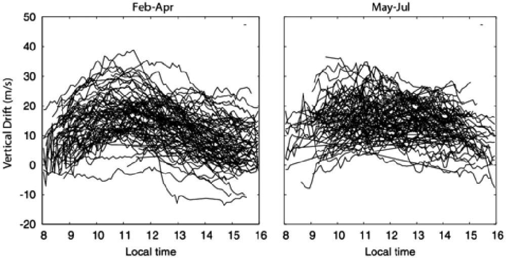
Variations in vertical plasma drifts measured at the magnetic equator from the Jicamarca Radio Observatory during periods of low solar activity. After Alken et al. [2009].

To establish the source of the variability in the daytime F-region ion drifts near the magnetic equator, we require knowledge of: (1) the neutral winds that can create dynamo electric fields throughout both the E- and F-regions (altitudes 100 – 300 km) above which winds are near-constant with altitude [cf. Rishbeth, 1972]; (2) the Hall- and Pedersen-conductance throughout the same region; and (3) the resultant high altitude electric field represented by the F-region ion drifts close to the magnetic equator. For item (1), this requires observations of the altitude profiles of the winds, which can only be obtained via limb-viewing remote-sensing instruments. For item (2), the E-region conductance in the low-latitude, daytime region is dominated by photochemistry that can be modeled accurately and validated with daytime O⁺ density retrievals and assimilative modeling, specifically using IDA4d [Bust et al., 2004; Bust and Datta-Barua, 2014]. For item (3), because magnetic field lines at F-region altitudes can be considered equipotentials, the electric field and associated ion drifts can be observed at any point along the same magnetic field line above the dynamo region (‘above’ being ~300-800 km altitude). Thus, it is vital for ICON to observe the neutral wind over the altitude range of the dynamo region (~100-160 km) and ion drifts at F-region altitudes in such a way that the two measurements are made on the same magnetic field line, and within a time-range that is small compared to the characteristic time-scale of the variability shown in Figure 1. As the winds can only be observed over this range using remote-sensing limb observations, the simultaneous observation can only be achieved via a combination of in situ determination of the electric field at the spacecraft with the remote-sensing of the winds on the limb. ICON determines the electric field by measuring with an Ion Velocity Meter (IVM) the local ion drift, which for F-region altitudes is directly related to the E-field. For locations close to the geomagnetic equator, these geometric requirements can be met, as described in the caption to Figure 2.

Fig. 2.

The unique observational strategy of ICON is illustrated in a pass of the spacecraft where its combined measurements give a complete characterization of the dynamical coupling between the daytime ionosphere and thermosphere. The three locations of the illustrated spacecraft indicate steps in the orbit over a total of ~7 minutes. The image of the daytime ionosphere is obtained in the region where the line-of-sight wind speed observations cross.

Near the dip equator, the geomagnetic field line curves down away from the spacecraft with a radius of curvature approximately equal to half the radius of the Earth. From this vantage point, tangent points on the limb of the wind observations made at 45° and 135° in azimuth relative to the spacecraft orbital track (necessary to provide vector wind measurements) descend similarly, nearly tracking the magnetic field. This figure thus describes the required viewing geometry obtained within a few degrees (~10°) of the geomagnetic equator. As long as all measurements are made, a view either north or south from the observatory will meet this viewing geometry requirement. The IVM instrument needs to be ram-facing to make this measurement, but as noted later, ICON carries two IVM heads separated by 180°, supporting complete scientific measurements for both north and south facing views.

2.2. Science Objective 2: How do large-scale atmospheric waves control the ionosphere at low latitudes?

It is now understood that large-scale waves generated in the lower and middle atmosphere may propagate upward and into the upper mesosphere and lower thermosphere (MLT). Furthermore, in the MLT, such waves are the dominant source of wave energy, though expected to dissipate at altitudes above ~140 km. Corresponding wave structures in the plasma have been observed throughout the low-latitude ionosphere reaching up to heights of 800 km [Hartman and Heelis, 2007]. One of the clearest examples of this is shown in Figure 3, where there is a close correspondence between tidal signatures at 115 km and ionospheric densities several 100s of kilometers higher. ICON will resolve fundamental questions about the coupling mechanisms between these two regions that drive similar-scale wave patterns and quantify the relative importance of (1) changes in the wind-driven electrodynamics; (2) changes in the conductance; (3) changes in neutral composition; and (4) direct forcing of the ionosphere by those large-scale atmospheric waves that actually propagate to higher altitudes. To do this, ICON must measure (1) the physical parameters that are directly associated with atmospheric waves: neutral winds, temperature, density, and composition, all as a function of altitude, local time and geographic location; (2) ion drifts on field lines co-located with (1); and (3) ionospheric density profiles, with coverage to match (1) and (2).

Fig. 3.

Longitudinal variations in the nighttime FUV brightness of the equatorial ionospheric anomaly compared to the amplitude of predicted temperature variations driven by non-migrating diurnal tides at the equator. The FUV emissions originate from the F-layer of the ionosphere above 300 km (from IMAGE FUV (black) and TIMED GUVI (red)), while the temperature amplitudes from the Global Scale Wave Model are shown at 115 km (blue). After Immel et al., 2006.

Exciting results from recent work have shown a striking resemblance between the large-scale structure of the equatorial ionosphere and tides in the lower thermosphere [see England (2012), for a complete review]. Solar thermal tides (as distinct from lunar gravitational tides) are atmospheric oscillations with periods that are sub-harmonics of a solar day. They are forced by processes connected with the diurnal cycle of heat release in the lower atmosphere. The daytime heating of Earth’s surface by sunlight, absorption of solar radiation by ozone, and the release of heat by the condensation of water vapor in convective clouds are the major drivers of tides. Migrating tides are westward propagating waves which follow the apparent motion of the sun [Forbes, 1995]. Thus they are typically linked to the diurnal cycle of radiative heating by, for example, ozone in the stratosphere. By contrast, nonmigrating tides are linked with latent heat release from deep tropical convection which is preferentially associated with specific geographic regions, but which also varies diurnally. These oscillations propagate up from the lower atmosphere to the thermosphere where they drive large wave patterns in the winds, temperatures and composition.

Through these changes, it is believed that these waves are able to drive the motion, production and evolution of the ionosphere at low latitudes, creating a coupling between our tropospheric weather system and the upper atmosphere and near-space environment that is stronger than previously determined. Following the paper that discovered clear signatures of this coupling by Immel et al. [2006], a number of recent studies have observed what appears to be tidally induced variability in the ionosphere and thermosphere: total electron content [Lin et al., 2007], vertical ion drifts [Hartman and Heelis, 2007; Kil et al., 2007], neutral winds throughout the thermosphere [Lühr et al., 2007; Talaat and Lieberman 2010], thermospheric O/N₂ [Zhang et al., 2010], and ionospheric electrojet currents [England et al., 2006b]. Each of these studies has identified a possible mechanism or pathway to produce the effect. However, it is simply not known how the wave signature in the atmosphere is impressed upon the ionosphere.

A study by England et al. [2010] examined four of the proposed pathways described in the above noted research. At present, we do not have measurements sufficient to rule out any of these four, or to determine how much of the longitudinal variability in the ionosphere can be attributed to each one of these. The only way to evaluate the competing influences is to simultaneously observe the key, unique features associated with each of these pathways along with the resultant ionospheric structure. In particular, these observations must be in the 100-300 km altitude region where the coupling mechanisms are believed to operate most effectively. ICON will provide the necessary measurements of winds at E- and F-region altitudes, conductivity, and chemical composition in order to identify the key drivers and understand how they may combine to produce the observed effects. Since each of the main tides in the thermosphere peak at different times of year, it is important that such observations be made at an appropriate cadence and duration to resolve the dominant mechanisms as they change throughout the year. ICON provides the measurements and coupled models necessary to carry out exactly such a study.

Central to ICON’s ability to address Science Objective 2 are its observations of atmospheric tides. Atmospheric tides are global-scale atmospheric waves with periods of 8, 12 and 24 hours, typical vertical wavelengths of ~20-30 km in the lower thermosphere (increasing with altitude to be quasi-infinite in the upper thermosphere) and horizontal wavelengths of integer fractions of the circumference of the planet (of order 60-360° in longitude and 30-90° in latitude). While the amplitudes of these waves can vary with season, previous observations of these waves in the mesosphere and lower thermosphere have shown that the dominant tidal waves persist for several months at a time, allowing good characterization of their properties by an observatory that can collect the adequate data in a period of time as long as a month. Specific requirements for tidal observations are discussed in Section 3.2.

2.3. Science Objective 3: How do ion-neutral coupling processes respond to increases in solar forcing and geomagnetic activity?

Remarkable changes in the ionosphere and thermosphere occur at low latitudes in response to disturbances in the solar wind. The electric field induced by the solar wind directly competes with internal drivers (Science Questions 1 and 2) and dynamo fields driven by storm-time neutral winds. Without comprehensive measurements of all the local drivers and the response of the ionosphere/thermosphere system, we depend upon numerical models to best understand the effects of these competing processes. ICON will provide the set of measurements that will allow for the first time a complete separation of internal “wind/wave-dominated” forcing from external “storm-driven” disturbance processes to understand how these processes interact to form the response of our ionosphere to storm inputs.

During periods of low magnetic activity, tidal forcing and other wave effects routinely shape the ionosphere (see Science Objectives 1 and 2). However, at enhanced levels of solar and geomagnetic activity the ionosphere changes on a global scale under the influence of EUV flare inputs [Immel et al., 2003; Sojka et al., 2013], storm-time electric fields [Tsurutani et al., 2004], and global modification of thermospheric neutral wind and composition [Fuller-Rowell et al., 1991; Immel et al., 2001]. ICON will be launched in the declining phase of solar activity, and will observe the ionosphere-thermosphere system affected by these inputs with a range of intensities. It will observe the modification of the equatorial ionosphere as it evolves from wave-dominated to storm-driven, a transition that is surprisingly complex and poorly understood, largely due to the absence of coordinated, simultaneous measurements such as those that will be made by ICON.

With the arrival at Earth of a large southward transient in the solar wind’s magnetic field, penetrating electric fields can lift the ionospheric plasma all across the dayside [Kelley et al., 2010]. These effects decline as shielding by inner magnetospheric current systems becomes more effective, a process that can take an hour for low- moderate activity (Kp~3) [Earle and Kelley, 1987] or longer for more energetic events [Huang et al., 2010]. The elevation of the F-layer significantly reduces ion drag, an effect that models predict will allow F-region neutral winds to increase across the dayside [Fuller-Rowell et al., 2002]. This buildup of momentum in neutral winds should develop at all local times, thus modifying the dynamo action of the F-region that is most effective at night [Heelis, 2004]. At the same time, the F-layer is potentially enhanced for the fact that its uplift reduces chemical recombination. When the denser layer does settle, ion drag on the neutral winds exceeds the initial condition. Thus, a “simple” action near noon drives a complex system with feedbacks that must be quantified before the non-linear ionospheric response to external forcing can be understood and predicted. ICON will monitor all aspects of these processes as a geomagnetic storm progresses.

Furthermore, with prolonged activity, the high-latitude effects of the solar wind disturbance drive a temporary neutral wind dynamo at lower latitudes that builds a dusk-to-dawn electric field that usually opposes the normal dynamo field [Blanc and Richmond, 1980]. These types of electric field disturbances extend from high- to low-latitudes over the hours of the disturbance epoch. ICON will be the first mission to simultaneously measure both disturbance electric fields and neutral winds and their effects on the densest plasma in geospace, the low-latitude ionosphere.

Extensive modeling of the coupled behavior of the ionized and neutral gases has provided significant insight into the processes at work [e.g., Maruyama et al., 2007]. The competing effects of penetrating electric fields and the disturbance dynamo have been evaluated using models, the latter of which, for instance, greatly reduces zonal winds in the post-sunset region from typically large eastward values (see Figure 4). However, recent results from incoherent scatter radars show that penetrating fields may actually reduce F-layer heights in this sector and therefore also slow zonal flow through increased ion drag [Kelley et al., 1989]. Direct observations of F-region winds and ionospheric heights in this region are required to unravel the relative importance of these competing effects. Furthermore, any effort to quantify these effects must properly account for the strong tidal and wave-forced “internal” variability that could otherwise be mistaken as temporal variability introduced by external agents.

Fig. 4.

Vectors show the difference in wind direction at 400 km altitude between a quiet and active run of a global I-T model from Maruyama et al. [2005], where colors indicate changes in total electron content. Post-sunset zonal winds are highly reduced from their normal eastward flow. Is this due to ion drag from the lowered F-layer or to disturbance winds from high latitudes?

The spatial, temporal and precision requirements for measurements of neutral winds and composition, plasma density and velocity taken to meet Science Objectives 1 and 2 are also stringent enough to characterize geomagnetic storm effects (as discussed in Section 3.3). In meeting Objectives 1 and 2, ICON will obtain the baseline characterization of the internally driven non-linear coupling between these neutral and ionospheric parameters that will be used to validate the ion-neutral physics simulated in the coupled ICON numerical models. During periods of enhanced solar and geomagnetic activity, ICON will determine how these parameters deviate from their baseline and will relate them to the strength of the solar-wind electric field forcing that is externally applied to the global ionosphere-magnetosphere system. Characterization of the external forcing will be derived from the AMIE assimilative model, which can provide a robust specification of the geo-effective cross-polar-cap potential (CPP) and other key parameters through assimilation of ground-based data, aided by direct measurements of the solar wind velocity and IMF or radar data (as available). By comparing the temporal behavior of the disturbance-driven components of the low latitude thermospheric and ionospheric responses with the development of the CPP, ICON will determine the relative importance of the drivers during different phases of increased geomagnetic activity.

3. Science Requirements

The ICON science requirements are developed such that the observatory may successfully achieve the scientific objectives described in the previous section. In the development of the requirements, the state of knowledge of the ionosphere-thermosphere system is reviewed, and the type and precision of measurements needed to fully address the objective is established. Through addressing the common needs of the three objectives, ICON’s requirements are reduced to a set that meets all science demands.

3.1. Requirements for Science Objective 1

As noted in the description of Objective 1 in Section 2.1, ICON must determine the neutral winds in the altitude region where they effectively generate dynamo electric fields, the altitude profile of conductivity throughout the same region; and the F-region ion drifts close to the magnetic equator. To provide sampling over the altitude range required, (1) and (2) can only be obtained via remote sensing, whereas (3) can be obtained in situ from low-Earth orbit. These measurements can be compared scientifically in the geometric configurations described in the Science Mission Design (Section 6.3)

Figure 5 shows a survey of one month of data from C/NOFS CINDI [Heelis et al., 2010] showing the typical variability seen in the daytime ion drifts during quiet periods. While the instrument is sampling at scales down to seven km in-track, the strongest variability is seen at scales of 800 km or more (note, this is quite different from the scales of instabilities that can dominate such a spectrum at night). Structures of this scale are generally associated with tides or planetary waves, generally propagating eastward or westward with velocities much smaller than the C/NOFS observatory. Thus, to establish the origin of this variability, ICON must sample the wind and conductivity parameters (1 and 2) at horizontal scales of 500 km, while measuring the related vertical drifts (3) at this resolution or better. These scientific measurement requirements define the instrument requirements regarding temporal and spatial resolution.

Fig. 5.

Spectral analysis of vertical drifts measured by C/NOFS-CINDI close to local noon, magnetic equator. Power spectrum for 1 month of data is shown. Almost all the power in the spectrum is for variations with horizontal scale sizes over 800 km (sampling frequency < 0.01 Hz), thus ICON is designed to observe the variability of the drivers chiefly of this scale and larger. Given orbital velocity, 1 Hz ~ 8 km.

Typical wind perturbations associated with large-scale waves in the daytime lower thermosphere are not expected larger than ±60 ms⁻¹ [cf. Hagan and Forbes, 2002], so to provide measurements with adequate resolution for comparison to ion drifts (say 6 range bins) ICON must measure winds with a per-sample precision better than 20 ms⁻¹. To determine if variations in the conductivity are able to produce the observed variability in the ion drift, ICON must measure the electron densities in the F-layer with a precision better than 20%, where the peak density (NmF2) can vary by a factor of 2. The height of the F-layer (hmF2) can vary by 100 km, and this height should be determined to better than 20 km. The related conductivity profiles are then determined using the IDA4D. The variability in the ion drifts can result in values during quiet times over a range of −30 to +30 ms⁻¹. For the equivalent number of range bins as the wind measurements, precision of 10 ms⁻¹ per sample of the plasma motion is needed to make comparisons with the winds and conductivity products. These requirements drive aspects of the observatory fine pointing capability, many aspects of the instrument design, and for the remote sensing instruments, the performance of the retrieval algorithms.

The daytime E-region wind dynamo is the target for these measurements, specifically in those regions magnetically connected to the higher altitude plasma observations. The winds in the E-region, from 100-160 km altitude, can be expected to change significantly with altitude. However, this assertion is based upon nighttime wind observations [cf. Larsen, 2002], and there are in fact very few daytime wind measurements in this altitude range. Though the nighttime E-region exhibits wind shears with reversals on scales of a few km, this is in the absence of strong drag from the daytime E-region plasma. Further, the dynamo fields originate in the convolution of those winds with a conductivity profile that in daytime varies more regularly with altitude [Richmond, 1995; Heelis, 2004]. In light of these facts, wind measurements with height resolution of 10 km obtained simultaneously over a range of altitudes that comprise the daytime dynamo region will provide a profound advance over any previous effort. Conductivity profiles must be determined on these scales as well. These requirements drive the spatial resolution of the remote sensing wind instrument, and the performance of the wind retrieval.

3.2. Requirements for Science Objective 2

To measure large-scale atmospheric waves and tides and their effects on the ionosphere, ICON must measure (1) the physical parameters that are directly associated with atmospheric waves: neutral winds, temperature, density, and composition, all as a function of altitude, local time (LT) and geographic location; (2) ion drifts on field lines co-located with (1); and (3) ionospheric density profiles, with coverage to match (1) and (2).

The most important observations are those of atmospheric tides in the neutral atmosphere. These waves have typical vertical wavelengths ≥20 km in the lower thermosphere (increasing with altitude to be quasi-infinite in the upper thermosphere) and horizontal wavelengths on the order of 2000 km. The resolution of the observations in (1) must be a fraction of these wavelengths (1000 km is adequate, 500 km is ideal). Each of these parameters must be measured with sufficient sensitivity to capture the tidal perturbations of the atmosphere.

Prior to discussing the specific measurement needs, it is important to consider the competing needs to provide good characterization of the tides at low to middle latitudes while maintaining the highest precession rate possible for rapid sampling of all combinations of latitude, longitude, and LT. The precession rate of a satellite in a circular orbit about Earth is reduced as orbital inclination increases, but the breadth of latitudinal sampling is of key importance as well. For example, an equatorial (0° inclination) mission could only provide the most limited information on tides, given the single latitude of observations.

An investigation of atmospheric tides and their effects at low latitudes can be achieved from a range of orbital inclinations. The 27° orbital inclination, described earlier for Objective 1, falls in this range, as described in the companion paper [Forbes et al., this issue]. This inclination provides access to a required range of latitudes and is sufficiently low to provide the rapid precession rate required for sampling all locations and LTs within one month (27-day half-precession @ 575 km circular orbit). Tidal parameters will be obtained from the ICON observations using Hough Mode Extensions [HME; Forbes and Hagan, 1982]. ICON will provide winds and temperatures sufficient to constrain the leastsquares fitting of each of the Hough modes to accurately retrieve the tidal components in the lower thermosphere and up to 400 km altitude for investigations of direct forcing of the F-layer. ICON fully specifies the tides that are critical to measure for equatorial science in less than half the time of the progenitor mission TIMED (that mission having a ~60-day half-precession period).

Typical tidal amplitudes in the region of interest are of order 10 ms⁻¹ and 20 K [Hagan and Forbes, 2002], implying specific measurement requirements that are determined below. First, consider the case of a TIMED-like 60-day full sampling period and define the spatial and temporal sampling bins that would be required to resolve any tides present. Given the vertical wavelength of tides as discussed above, winds and temperatures should be sampled with height resolution of 5 km. Representative latitude x longitude bins of 5°×15° and one hour of LT would be adequate to resolve tides, where multiple samples in each bin reduces the uncertainty in the wind and temperature to be fitted. Our orbit provides a minimum of 12 samples per bin for the winds and 24 for the temperatures. At each latitude, spatial-temporal fits are then made over all LT and longitudes (e.g. in the case of the wind, this fit involves ~5,000 samples). Thus, to achieve the 5 ms⁻¹ and 5 K requirement in measuring the tides over 60 days, the instrument must measure with a precision of 17 ms⁻¹ and 22 K per sample. Because the derived quantities are wave properties, rather than the absolute wind and temperature structure, there is no requirement for absolute accuracy beyond that the zero-wind determination cannot drift more than 2 ms⁻¹ in any n-day window (where n> 27 days for ICON).

For the shorter temporal resolution period of 27 days, and assuming smaller spatial bins of 5°×5°, the requirements are more stringent, with a precision of 8.7 ms⁻¹ and 12 K per sample, with a minimum of 3(6) samples per bin of velocity(temperature). Given the growing interest in understanding the temporal variability of tides at timescales better than 60 days [cf., Pedatella et al., 2016], ICON will provide new and much needed measurements of this phenomenon.

It is worth noting that throughout the discussion of the requirements for Science Objective 2, the requirement is stated in geophysical units, averaged over a spatial-temporal bin of a particular size. This is only used as a means of translating the requirement from the science objective to the instrument measurement requirements. No actual binning is used in the actual scientific analysis (the full spatial and temporal resolution available are used) and as such the size of the bin stated is of no consequence other than in helping translate the science requirement (e.g. the tidal spectrum from 60-days of observations) into a per-measurement instrument requirement. The performance of HME fitting routines that are constrained by data in the ICON sampling range is shown in Fig. 6. In comparison to HMEs that are constrained by a complete global set of observations, the fits to the limited range of data are, in this example, realistic. A broader set of tests is performed in the companion paper to this report [Forbes et al., 2017, this issue]

Fig. 6.

a,b,c Observing System Simulation Experiment of HME fitting routine to retrieve tidal components of the temperature field at the local time of noon. The temperature at the noon meridian at 100 km altitude predicted by the TIMEGCM for a 24-hour period is shown in Figure 6a. Temperatures reconstructed from an HME fit to the TIMEGCM wind and temperature fields using global sampling in the 90-105 km altitude range are shown in Figure 6b. Temperatures from the HME fit constrained only by data in the −12 to +42 degree latitude range (simulating ICON’s orbit and views) are shown in Fig. 6c.

To quantify further effects of tidal forcing, two parameters are measured: (1) the neutral composition changes that tides induce [Roble and Shepherd, 1997] and (2) the vertical ion drifts they impose by their modulation of the E-region dynamo [Hagan et al., 2007; Kil et al., 2007]. The composition changes (O/N₂) are measured during the day where their importance to the ionospheric production rate is greatest. The tides studied have been reported to produce changes in O/N2 of order 10% [Zhang et al., 2010], thus our requirement is to measure this ratio to 5% per 27 days (8.7% per 500 km). Vertical ion drifts are measured during day and night to study both electrodynamic and direct forcing of the ionosphere by tides. Previous observations have shown this varies by around 10-20 ms⁻¹ in response to tides, so our measurement requirement is a precision of 10 ms⁻¹ on scales of 500 km.

The time-integrated effects of photochemical and electric field forcing on ionospheric densities must be directly measured in the ionosphere. Altitude information is critical to observe the coupling between different layers and the development of these signatures throughout day and night. The key parameters of height and density of the F-layer, hmF2 and NmF2, can be retrieved from altitude profiles of dayside extreme-ultraviolet (EUV) 83.4 nm and nightside far-ultraviolet (FUV) 135.6-nm emissions. Previous observations have attributed changes as large as 40 km in hmF2 40% in NmF2 to tidal forcing [cf., Lin et al., 2007]. For adequate resolution in these ranges, therefore, measurements must have height resolution of 20 km or better, and sensitivity to retrieve NmF2 to at least 20%.

Primarily for this objective, ICON supports an atmospheric/ionospheric modeling effort to capture the dynamical forcing from the lower and middle atmosphere and simulate the effects at higher altitudes and in regions away from the ICON measurements. Two physical models are used for this: the TIEGCM [Maute, 2017, this issue; Richmond et al., 1992] and SAMI3 [Huba et al., 2017, this issue]. The TIEGCM lower boundary conditions are, in part, specified by the HME fits to measured winds and temperatures as discussed above. The signature of the tides at higher altitudes can be observed directly and compared to the TIEGCM wind and temperature fields as a validation of this process. Further, the TIEGCM neutral atmosphere (winds, composition, and temperature) will be passed to the SAMI3 model to provide a realistic environment for the simulation of ion chemistry and electrodynamics from the E-region to the plasmasphere with high spatial resolution. This modeling framework provides a capability to investigate the relative importance of winds, electric fields and changes in neutral composition on changing ion density.

3.3. Requirements for Science Objective 3

To evaluate the coupled behavior of the I-T system during periods of enhanced solar and geomagnetic activity, ICON will operate with a high operational efficiency to make continuous observations of conditions during which Kp rises to values of 5 or more. With launch planned for November 2017, it is expected that ICON will encounter ~4–8 such events in its first 12 months of operations which is sufficient to establish the change in the underlying ion-neutral coupling during these periods. The effects of these events last for ~3-24 hours, so rapid sampling of all local times (total LT coverage in 2 hours) is required.

Objective 3 will be addressed using simulations from the TIEGCM/SAMI3 models (described above for Science Objective 2) that are both constrained by and compared to ICON’s observations. These models are constrained at their lower boundary by the atmospheric tides ICON will measure (as addressed by meeting Objective 2) and at high latitudes using the AMIE assimilative model. AMIE produces high latitude potential maps that are constrained using all available data sources such as ground-based magnetometer networks, radars and solar wind monitors when available. Solar wind measurements are expected to be continuous during the ICON mission, with new assets committed to providing these [e.g. DSCOVR (Burt and Smith, 2012)]. The TIEGCM/ SAMI3 models require AMIE output at 5-minute cadence, which will be produced for the entire ICON mission and provided as a mission data product. To observe the motion of the F-layer in response to external forcing, ICON must measure (1) the low-latitude E×B ion drifts and (2) the height of the F-layer (hmF2) both day and night. Typical storm-time changes in the ion drifts are shown in Fig. 7. Recent measurements [Kelley et al., 2010] suggest more complex responses, such as where pre-reversal enhancement drifts may be reduced or even turn negative, while the daytime drifts remain upward during active times.

Fig. 7.

Mean vertical drift as a function of local time under quiet (case 0) and disturbed (case 2) electric field inputs prescribed by the Rice Convection Model [Toffoletto et al., 2003], after Huba et al. [2005]. The pre-noon maximum in upward drift corresponds to a peak in plasma production, while the 18 MLT peak is the pre-reversal enhancement.

ICON must measure these responses with a precision of 10 ms⁻¹ in order to identify their perturbation from quiet times. For changes in hmF2 to have any impact on the neutral winds, they must be on the order of a neutral scale height (~40 km in this region), so these must be measured with a precision of 20 km. To separate the effects of photochemistry from transport in changing the F-layer, ICON must also measure (3) the neutral composition (O/N₂) during the day when ions are produced. Perturbations in O/N₂ must be larger than those produced by atmospheric tides to produce any noticeable effect. Finally, to observe the changes in the winds from the reduced ion drag or disturbance winds, ICON must measure the horizontal neutral winds at F-region altitudes in both daytime and at night.

Figure 4 shows the typical wind perturbations expected, which would be well represented if ICON measured the winds with a precision of 10 ms⁻¹ in the F-region. For this objective, all requirements are in terms of precision. There is no accuracy requirement, as the absolute value of any parameter at any one time is not sought, but rather simply its change in relation to changes in geomagnetic activity.

Advances can be achieved by comparing the TIEGCM/SAMI3 models with the ICON observations. Specific conditions and behaviors of the system during each storm period can be evaluated, and attributed to aspects of the larger-scale/global storm response. Departures from modeled parameters can be evaluated in terms of the phenomena present regionally (e.g., pre reversal enhancement, daytime “superfountain”). Modifications of the free model parameters (e.g. eddy diffusion) can be tested if needed, offering a potential pathway for model improvements. Analyzing these final model runs with equivalent quiet-time simulations will enable us to identify departures in the I-T system associated with enhanced solar wind and geomagnetic activity. These simulations, combined with the capabilities necessary to address Objectives 1 and 2, fully describe the data and analysis required to also address Objective 3.

3.4. Science Requirements Summary

The science requirements for all three objectives discussed above were reviewed to determine the most stringent requirements for each measurement, and the results collected in a Program Level Requirements Agreement held by NASA. Table 1 summarizes these measurement precision requirements (last column) as Level 1 (L1) requirements. The table also reports the Level 2 (L2) requirement that the ICON project systems and instrument teams worked to meet during design and development phases of the mission, and verify before delivery. This established performance margins of 200-300% as the design and build of the instruments and spacecraft proceeded, and retrieval algorithms were developed. The L2 requirements reported in Table 1 are relaxed from the original values held for MIGHTI and IVM for the fact that during development, component testing or retrieval development efforts better informed performance predictions. Treating the established margins as performance reserve to the established L1 requirements gave project system engineering direct insight to the observatory performance during all mission phases. As is reported in Section 6.2, the observatory is predicted to meet these L2 requirements stated in Table 1.

Table 1.

Science requirements for the ICON mission. The ICON baseline mission meets all of these requirements. Nighttime requirements extend only to midnight. The threshold mission is enabled by meeting requirements SR-1,2, and 6. At launch, the ICON observatory has the capability to meet the baseline mission and Science Requirements SR-1 through SR-5, and the Science Operations Center is prepared to generate products identified in SR-6 and SR-7.

Program Level (L1)* Science Requirements for ICON
Altitude and Precision values reported at both Level 1 and Level 2
Label	Science Requirement Statement	Day/ night	Altitude L1,L2 (km)	Vertical Res.	Precision L1,L2
SR-1	ICON shall determine altitude profiles of upper atmospheric wind vectors on the limb with a horizontal range resolution of 500 km great circle.	Both	95-105, 90-105	5 km	16.6, 8.7 ms−1
		Day	105-150,105-170	5 km	16.6, 10 ms−1
		Day	N/A,170-200	30 km	16.6, 10 ms−1
		Night	220-280, 200-300	30 km	16.6, 8.7 ms−1
SR-2	ICON shall provide a measure of the vertical ion drift velocity component perpendicular to the magnetic field with horizontal range resolution of 250 km great circle.	Both	In situ		10, 7.5 ms−1**
SR-3	ICON shall measure the peak ion density of the daytime and nighttime ionospheric F-layer with horizontal range resolution of 500 km great circle.	Both	@ F-layer peak		20, 10%
	ICON shall measure the altitude of the layer peak with horizontal range resolution of 500 km great circle.		N/A		±20, ±10 km
SR-4	ICON shall determine altitude profiles of upper atmospheric temperature at a horizontal resolution element size of 5°x 5° latitude-longitude	Both	90-105	5 km	23.4, 12.2K
SR-5	ICON shall measure the altitude profiles of O and N2 to determine the column ratio of O/N2 in the daytime thermosphere with horizontal range resolution of 500 km great circle.	Day	130-200 km column		16.6, 8.7%
SR-6	ICON shall assimilate ionospheric measurements for determination of conductivity profiles coincident with limb measurements with horizontal range resolution of 500 km great circle.	Day	E- and F-Regions of ionosphere		10%
SR-7	ICON shall use geophysical models (eg. HME, TIE-GCM, SAMI3, AMIE) to support recovery and determination of the following parameters: Atmospheric Tidal Amplitude and Phases, Coupled Ionosphere-Thermosphere parameters, and High latitude Potential Distribution.	Both	E- and F-Regions of ionosphere		No Specification

^**for ICON orbit, corresponds to 5.5 and 21 ms⁻¹ cross-orbit-track and in-orbit-track velocity precision, respectively, in worst case magnetic/orbital geometry.

4. Science Instruments

4.1. Michelson Interferometer for Global High-resolution Thermospheric Imaging (MIGHTI)

The MIGHTI instrument is supplied by the Naval Research Laboratory (NRL). It can measure the wind velocity and temperature of the upper atmosphere with observations on Earth’s limb [Englert et al., 2017, this issue; Harlander et al., 2017, this issue]. Wind speed is measured by interpreting the Doppler shift of the atomic oxygen red and green lines (630.0nm and 557.7nm) [Harding et al., 2017, this issue]. Temperature is measured from the spectral shape of the molecular oxygen band at 762 nm [Stevens et al., 2017, this issue]. The two identical sensors of the MIGHTI, MTA and MTB are mounted orthogonally and image the upper thermosphere to provide line of sight Doppler velocity measurements that can be combined to report vector winds versus altitude. A common Camera Electronics package, MTE, supports both of CCD imaging cameras used in MTA and MTB. A Calibration Lamp, MTC, provides an optical calibration signal to both MTA and MTB via a fiber optic connection. Finally, a stepper motor driver, provided by UCB, is included on each MIGHTI optical assembly. It provides an electrical interface between the MIGHTI aperture actuators and the Instrument Control Package (see Section 5.1). A model of MIGHTI is shown graphically in Figure 8. Aside from the components listed above, evident are the large radiators that draw heat from the actively cooled CCD cameras through heatpipes so they can be operated at −40°C in all solar illumination conditions. There is no “cold side” of ICON that provides continuous access of radiators to deep space.

Fig. 8.

The ICON MIGHTI Instrument

The MIGHTI instrument is one of two ICON instruments that has moving parts used regularly during flight. While the interferometers themselves have no moving parts, there are two apertures in each sensor that are motor driven. One aperture is at the rear of the baffle (sensor pupil), and the another aperture is an internal Lyot stop. Both apertures are operated simultaneously to provide an aperture reduction to 15% of the full aperture to improve stray light rejection during the dayside of the orbit, when the Earth’s disk is many orders of magnitude brighter than the targeted signal in the atmosphere, only 90 km above the bright surface. Specific details of this capability are discussed in the companion paper that describes the instrument in detail [Englert et al., 2017]. The specific design of the interferometer at the heart of the instrument is described by Harlander et al. [2017]. The principles and design of the retrieval algorithms for neutral winds and temperatures are described in this issue by Harding et al. [2017] and Stevens et al. [2017], respectively.

4.2. ICON Ion Velocity Meter (IVM)

The IVM is supplied by the University of Texas at Dallas (UTD). It will be used to determine the electric field perpendicular to the magnetic field and the ion motion parallel to the magnetic field through measurement of the ion drift velocity vector. Two full IVM instruments, IVM-A and IVM-B, are carried by ICON. Two sensors are part of each of these IVM instruments, the Retarding Potential Analyzer (RPA) and a Drift Meter (DM), which together provide data to determine the total ion concentration, the major ion composition, the ion temperature and the ion velocity in the spacecraft reference frame. A model of an individual IVM instrument is shown graphically in Figure 9. As shown in Section 5.2, these are mounted on opposite faces of the payload deck, pointed in opposite directions, providing the capability to meet threshold science goals if IVM and MIGHTI work together in either northern or southern-facing modes. Unlike the MIGHTI instrument, only one IVM will be powered and operated at any time in nominal science mode, IVM-A when EUV, FUV (see following sections) and MIGHTI are facing toward the northern hemisphere and IVM-B when they are facing toward the southern hemisphere.

Fig. 9.

ICON Ion Velocity Meter (IVM)

The full build and performance discussion of the instrument is reported in a companion to this paper [Heelis et al., this issue]

4.3. ICON Far-Ultraviolet Imager (FUV)

The ICON FUV instrument is a spectrographic imager [Mende et al., 2000; 2016], which produces 2-dimensional images of the scene in its field-of-view at two selected wavelengths with an approximately 5-nm passband with two separate cameras. The instrument will measure the brightness of both the 135.6-nm emission of O and the LBH emission of N₂ near 157 nm on the limb during the day. This provides the information necessary to determine the daytime thermospheric density profile of the neutral species O and N₂ and also provides radiance measurements required to determine the nighttime O⁺ ion density. Its design makes it completely blind to visible light while having a large aperture for FUV light.

A model of the FUV instrument is shown in Figure 10. The steerable turret contains a mirror which allows the reorientation of the field of view over ±30° in the horizontal plane, in 13 discrete steps separated by 5°. The instrument is provided with a digital image processing capability located in the Instrument Control Package (Section 5.1) to reduce the blur due to motion of the spacecraft during imaging integrations. This motion compensation, termed Time-Delay Integration (TDI) corrects for the apparent motion of features in the imaged scene, from disk views below the limb out to the furthest limb tangent points.

Fig. 10.

ICON Far-Ultraviolet Imager (FUV)

The FUV turret and TDI imaging mode are only operated at night, providing capability to image structure in the ionospheric plasma at the limb (at tangent points 1200-2000 km from the spacecraft). This capability allows FUV to identify regions of disturbed plasma densities that should be excluded from analyses of large-scale tidal forcing (Objective 2). The FUV instrument is described in a companion paper [Mende et al., this issue] and the function of the TDI feature is described in a second companion paper [Wilkins et al., 2017, this issue]. The retrieval algorithms for thermospheric composition and ionospheric densities are described by Stephan et al. [2017b, this issue], and Kamalabadi et al. [2017, this issue], respectively.

4.4. ICON Extreme-Ultraviolet Spectrometer (EUV)

The ICON EUV is a 1D imaging spectrometer [Bowyer et al., 1997] with a bandpass that allows it to measure the altitude intensity profile of ionized oxygen emissions (O⁺ 83.4nm and 61.7nm) on the limb in the thermosphere as well as the He 58.4nm line. It specifically is required to measure the bright 58.4-nm line to demonstrate that it is sufficiently separated from the dim 61.7-nm line. The instrument can hold pressure or a vacuum, is purged with inert gas or sealed up to launch, and has a one-time opening door that protects the open multi-channel plate that converts incident UV photons into pulses of electrons that are registered on the 2D crossed-delay-line detector [Lampton et al., 1987]. Major elements of the EUV imager are illustrated in Figure 11.

Fig. 11.

The ICON EUV Instrument

The instrument field of view intersects horizon, providing spatial resolution only in the vertical sense (with altitude), as the light is focused into a single vertical profile that is dispersed vs wavelength across the detector by the toroidal UV grating. As such, it provides the necessary emission profiles of two EUV emissions of O⁺ separately on the detector, and thus the information necessary to retrieve altitude-density profiles of the ion in daytime. Data collection is suspended in nighttime, though the electronics and high voltage power supply stay on to maintain a continuous thermal state. The complete description of the EUV instrument is provided in the companion paper to this report [Sirk et al., 2017, this issue], and the retrieval method is described by Stephan et al., [2017a, this issue].

4.5. Instrument Operations

The ICON imaging instruments change their operational state depending on whether the instrument imaging targets are in daylight or night. MIGHTI changes integration time between 30 (day) and 60 (night) seconds. In daylight, FUV lowers the intensifier gain and takes images in each of the two channels that are each binned into 6 vertical profiles per channel every 12 seconds, allowing 6 independent retrievals. At night, FUV takes both full TDI images and 6 binned profiles of the 135.6nm channel only (4x16km pixels) every 12 seconds. In order to obtain optimal images of ionospheric structures that may form during nighttime, the FUV turret is oriented such that the local magnetic meridian falls within the field of view. As noted above, EUV data are not collected at night, though the imager remains on. The spacecraft magnetic torque bars (MTBs), part of the attitude determination and control system, are only used when the observatory is 15 or more degrees of magnetic latitude away from the dip equator, and then only during 12 s of successive 32 s periods. This results in nearequatorial IVM data uncontaminated by torqueing fields, and at least 19s of uncontaminated IVM data every 32s away from the equator. The times of activity of the MTBs will be noted in the IVM data. A summary of these different states is provided in Table 2.

Table 2.

Instrument operating modes in Day and Night Mode. MIGHTI A/B modes will be synchronized to terminator crossings of the respective tangent point locations in the fields of view, and so will have differently timed modes changes (5-6 minute differences at each terminator crossing).

Sensor	Day Configuration	Night Configuration
MIGHTI A/B	30 s integration, 15% aperture	60 s integration, 100% aperture
FUV Channel 1 (135.6)	12-s integration, co- addition of limb samples in six vertical stripes	12-s integration in 6 vertical stripes, plus full TDI images of both limb and disc. Turret adjustment to local magnetic meridian in 5° steps between ±30°,
FUV Channel 2 (LBH)	12-s integration, with 6 strip co-addition as Channel 1	No data taken
EUV	12 s integration	No data taken
IVM A/B	1 s samples	1 s samples
Magnetic Torque Bars	12 s on / 20 s off outside of ± 15° magnetic latitude only	12 s on / 20 s off outside of ± 15° magnetic latitude only

4.6. Science Data Products

The four instruments of the science payload produce all of the observational data products of the ICON mission. Those products are listed below and their relationship noted in Figure 12. Each of these products from Level 1 to 4 will be available in NetCDF format.

Fig. 12.

The science data products for the ICON mission.

Level 0 are unprocessed outputs from the ICP. For MIGHTI, EUV and IVM, these are essentially direct outputs from the sensors, either CCD readouts (MIGHTI), electric currents (IVM), or integrated counts from the crossed delay line detector (EUV). FUV goes through additional processing steps, and direct CCD readouts are only provided in engineering modes.

Level 1 data from the remote sensing instruments are reported in calibrated radiances for EUV and FUV. For MIGHTI, interferogram phases and amplitudes and the relative brightnesses in the infrared channels are derived. For IVM, the arrival angles at the driftmeter are reported, as well as the current vs. voltage relationships determined in every RPA voltage sweep.

Level 2 products are retrieved geophysical parameters. For IVM, these require a calculation and conversion to plasma drift parameters in the frame of references of the rotating Earth [Heelis et al., this issue]. For the remote sensing instrument, these products all require the application of a retrieval algorithm to determine the geophysical parameters from the limb radiances. These retrievals vary in sophistication needed to meet the science requirements, and are discussed in companion papers to this one in this issue. [Stevens et al., 2017; Harding et al., 2017; Kamalabadi et al., 2017; Stephan et al., 2017 a, 2017b; all in this issue]. Level 3 products are daily summaries of the L2 products, and will likely be used to rapidly create browse products.

Level 4 products are outputs of the first principles and assimilative models that are regularly run to support the ICON science investigation. Outputs of all instruments are incorporated into the L4 products, by several pathways. The HME product incorporates temperature and winds from MIGHTI, which then informs the TIEGCM and subsequent SAMI3 model runs. Both daytime and nighttime ionospheric measurements are incorporated into the IDA4D assimilation, using the EUV L2 ionospheric profiles and the FUV L1 calibrated line-of-sight radiances directly.

5. Science Payload Design

5.1. Payload Control, Data, and Power

The power, commanding and data interfaces for all ICON science instruments reside in the Instrument Control Package, or ICP, which is provided by the University of California, Berkeley (UCB). It provides the electronic interface between the Spacecraft bus and the Instrument sensors.

The ICP consists of four boards illustrated in Figure 13. These boards provide the science payload all of its power, instrument control and data processing capability. The primary data interface for all instruments is provided by the Data Control Board (DCB). Data from the instruments is transferred to solid state memory on the DCB where an embedded processor implements all required algorithms for data handling/manipulation, as well as CCSDS-compliant packetization and eventual transfer to a solid state recorder in the spacecraft bus. The Power Control Board (PCB) is used to control power and monitor current to MIGHTI, IVM, MIGHTI Calibration Lamps and all the Payload operational heaters. A Low Voltage Power Supply (LVPS) powers the ICP itself and supplies switched, secondary power to the EUV and FUV instruments. The TEC Power Supply (TPS) provides software-controlled power to thermoelectric coolers within the MIGHTI cameras to chill the CCDs. Embedded software maintains the temperature of the CCDs at −40°C ±1°C using a proportional–integral control algorithm.

Fig. 13.

The ICON ICP, with four main boards in aluminum housings on a flexure mount, provide all necessary functionality for the 4 ICON science instruments, and a single point interface to the spacecraft. Unit is shown without a large flight radiator that attaches by the set of bolts to the LVPS.

The ICP provides all numerical processing for the payload, including the 2D FUV imaging mode that uses a Time-Delay Integration (TDI) algorithm to provide motion compensation during the accumulation of individual CCD readout frames at 8 Hz (100 frames co-added in 12 seconds) [see Wilkins et al., this issue]. It also implements the thermal control algorithms that maintain the MIGHTI interferometer temperatures in the narrow range (within <±0.1°C) necessary to minimize changes optical path difference within the interferometer due to both thermal expansion/contraction and refractive index changes of its components. The ICP therefore implements critical operational capabilities of the FUV and MIGHTI instruments, as well as for EUV and IVM, that are continuously used during science operation of the ICON payload.

5.2. Payload Mechanical and Thermal

The ICON science payload carries all of the science instruments and supporting harnessing and attachment points. The payload is integrated on a Payload Interface Plate (PIP) that connects physically to the spacecraft by three carbonfiber-based bipods. Each side of the PIP is populated with instruments and their supporting components, as well as spacecraft components consisting of 2 star trackers, the navigational magnetometer, and the S-Band antenna. The MIGHTI boresights are directed to provide two orthogonal lines-of-sight at a continuous tangent height approximately 1500 km from the orbital plane, which in the baseline configuration with IVM-A directed in the ram direction is to the port side, or north of the orbit track.

5.3. Payload Views and Pointing

From the vantage point of its planned 575 km circular orbit, the ICON remote sensing instruments are pointed toward Earth’s limb. Expected altitude ranges are reported in the companion papers for each instrument. The primary flight rule during science operations is to direct the bottom of the fields of view of both MIGHTI A and B to a tangent altitude of 90 km. This is performed regularly by the observatory, continuously correcting in pitch and roll for terrestrial nonsphericity and non-circular orbit, respectively. ICON is designed to meet its science requirements across the full range of potential observatory orbital altitudes from 450 km to 610 km, representing a 3-sigma orbit insertion error of the Pegasus launch vehicle. With a nominal orbit insertion in late 2017, ICON will likely be above 450 km for more than 10 years.

6. Observatory and Mission Design

6.1. Observatory Design

The ICON spacecraft is based on Orbital ATK’s LEOStar-2/750 platform, following the design established on missions such as GALEX, AIM, OCO, and NuSTAR but incorporating a new single avionics box called the Master Avionics Unit (MAU) that performs all Command and Data Handling tasks, controlling the Attitude Determination and Control Subsystem (ADCS) while also providing control of the Electric Power Subsystem. Its design supports all science requirements of the mission, meeting needs that include precise and stable pointing, rapid yaw maneuvers and ample battery power for all required observations during nighttime.

Upon deployment, the single solar array rotates once per orbit, maintaining the angle between the sun and the array normal at the minimum possible value. This rotation is not interrupted for any reason other than the case that the spacecraft enters safe mode, at which time the rotation is halted and the array normal is oriented toward the sun. The array is mounted away from the instrument FOVs, effectively eliminating glint from the panels as a source of stray light in the instruments, as illustrated in Figure 16.

Fig. 16.

The ICON observatory with solar array deployed

The observatory operates with no expendable propellants, maintaining attitude with 4 reaction wheels and 3 magnetic torque bars (MTBs). Its driving requirement is to implement specific series of yaw maneuvers in rapid succession, and to settle for science operations soon after the maneuver (see Section 6.4 for detail). Specifically, a 90° yaw must be completed in 150 s, including the time to settle to required observatory stability for science observations. All simulations and tests performed during ICON development and build show that the observatory meets these requirements.

The MTBs are a source of interference for the IVM measurements. Therefore, as noted in Section 4.5, no MTB operation is allowed within 15 degrees of magnetic latitude from the dip equator, and only in a 12/20 s on/off sequence at higher latitudes. Given this significant limitation in duty cycle, the ADCS for ICON is designed with a great deal of authority compared to other observatories of comparable size (285 kg). There are side-benefits to this besides performance margin in operational momentum unloading and magnetic dipole generation. For example, analysis shows that the atmospheric drag on the asymmetric observatory introduces a small torque, mainly in the yaw sense. The ADCS for ICON is easily able to counter this at any operational altitude of the observatory or conceivable atmospheric density profile. By this last point, it is expected that ICON will be able to provide the pointing performance required for scientific operations during periods of high solar activity and/or after an extended period of slowly decaying orbit.

The observatory is equipped with an S-band transceiver for communications. Observatory science and engineering data are stored onboard in a 2GB memory area and transmitted over an S-Band radio link to ground stations in 5-6 daily contacts at a data rate of 4 Mbps. The command uplink is also over S-band at 2 kbps. The expected volume of data generated by the observatory is approximately 1 GB per day.

The pointing requirements of the observatory are driven by the scientific performance requirements of the MIGHTI and IVM instruments. Only by maintaining precise control and knowledge of the observatory attitude can those requirements be met. The spacecraft carries a star tracker, provided by the Danish Technical University, equipped with two camera head units (CHUs) to meet these requirements, and can perform with either one of them occulted (i.e., with the sun near their field-of-view), or otherwise out of service. This is due in part to the availability of inertial data from the ICON spacecraft’s inertial measurement unit, that together with the un-occulted CHU can propagate position and pointing knowledge with precision and accuracy to meet science requirements through every expected occulted condition.

The payload deck and interface to the spacecraft must be stable under all solar illumination conditions, and so is constructed of aluminum honeycomb with carbon fiber facesheets and mounted to the spacecraft via three carbon fiber bipods. These design features support continuous science operations under the wide range of sun angles encountered by the observatory with every orbit, through every precession cycle and season.

6.2. Observatory Build

The ICON payload was integrated and tested for flight at Space Dynamics Laboratory in Logan, UT, including all harness and thermal blanketing. The ICON spacecraft was built, integrated and tested at Orbital ATK in Reston, VA, where the payload was received, and parts of the spacecraft subsystem added to it (S-band antenna, three-axis magnetometer, and both star tracker CHUs) before mating to the spacecraft. The observatory was at that point nearly complete, and ready for thermal blanketing and extensive rounds of performance testing and subsystem checkout. Full Observatory environmental testing was performed at the Orbital ATK spacecraft facility in Chandler, AZ. Figure 17 shows the complete observatory without the solar array in a 10k clean tent in Chandler. Covers on the CHUs are temporary and removed before encapsulation in the Pegasus fairing. Covers on MIGHTI A and B are also removed before flight (Cover A removed before fairing encapsulation, Cover B removed at the range just prior to launch).

Fig. 17.

The ICON observatory accompanied by Orbital ATK I&T leads in Chandler, Arizona in May, 2017.

6.3. Observatory Performance

As part of the verification of mission requirements, an extensive set of simulations of atmospheric and ionospheric conditions was performed, as described in the number of papers in this issue describing the retrievals. A summary of the performance of the observatory is provided in Table 3. These are the best available estimates before launch, and will be held against the required performance after observatory checkout (Launch + 30 days).

Table 3 –

Expected Observatory Performance by Instrument. Altitude resolution and precision for each measurement by ICON is provided, including uncertainties originating with pointing errors. MIGHTI measurement precision for winds and temperatures is determined for retrievals with the described vertical resolution (roughly half the vertical imaging resolution). In contrast, instrument vertical resolution is reported for the retrievals of key ionospheric/thermospheric parameters using the FUV and EUV, noted with asterisks.

A key requirement of the spacecraft is to provide pointing information for the payload with high precision and accuracy. Pointing errors can result in incorrect removal of spacecraft velocity from the remotely-retrieved wind or the in-situ plasma drift measurements. As such, the spacecraft is required to provide 3σ pointing accuracy and precision of 142 and 86 arcsec, respectively, in all three rotation axes. Analysis shows that in worst case conditions, the spacecraft exceeds these requirements, providing performance margins of 40 and 18% respectively.

6.3. Science Mission Design

ICON’s design allows it to make observations necessary to address its 3 science objectives, measuring the key parameters that influence the coupling of the ionosphere and thermosphere. In any 7-minute period it makes all of these measurements, including the neutral wind altitude profiles that are so crucial for understanding the variability of the ionosphere.

ICON will only spend some fraction of any of its (nominally ~94.8 min period) orbits in the geometry shown in Figure 18, where the observatory is in the immediate vicinity of the apex of a magnetic field line. On average during a day, this fraction is a basic function of orbital inclination. A study of the effect of orbital inclination is summarized in Table 4. For latitudes equatorward of ~15°, ICON would not cross the magnetic equator at every longitude, thus no inclination below 15° is acceptable for complete equatorial coverage. At inclinations higher than ~30°, the time ICON spends in this region drops below 100 minutes per day, which would still permit the investigation required for Science Objective 1, but is less than ideal. The length of time per orbit that ICON remains in the required viewing geometry is also an important consideration. Because daytime data primarily between 9-15 hours LT are used for Science Objective 1, each daytime pass must be considered in isolation. Thus, the longer ICON spends per orbit in the required viewing geometry, the better gradients and spatial scales of variability can be determined. Table 4 shows that the maximum duration decreases by a factor of 2 going from 15 to 27° orbital inclination, and is further reduced by another factor of 2 going from 30 to 45°. From this information, the optimum orbital inclination to address Science Objective 1 alone would be seen to be between 0-15°, and no higher than 27°. However, the importance of Science Objectives 2 and 3 further weigh on the selection of orbital inclination for ICON. These latter objectives require middle latitude observations, and so higher inclinations. For these reasons, the inclination of ICON is selected in the high end of the acceptable range for Objective 1. Notably, inclinations of 54° and larger never provide the geometry to make comparable observations for Objective 1, and near equatorial orbits will never provide data that would allow specification of atmospheric tidal components for Objective 2.

Fig. 18.

Geometry of the ICON observations required for Science Objective 1. ICON is shown near the magnetic equator. At position T=0, FUV and EUV instruments view the limb thermosphere/ionosphere (fields of views shown in light blue) while the IVM measures the in situ ion drift, representative of the electric field present on the field line (red arrows). MIGHTI (fields of view shown in light red) measure the relevant wind vector components (yellow) at positions T-3.5 min and T+3.5 min. The tangent point locations where MIGHTI samples the wind field vary with altitude following closely the Earth’s dipole magnetic field line that is intersecting the spacecraft at the T=0 position.

Table 4.

The effect of varying ICON’s orbital inclination on the length of time per day and per orbit that ICON is in the orbital viewing geometry for Objective 1.

Orbital inclination	Optimal geometry per day	Maximum duration single orbit
0°	330 min	45 min (0 min in S. American sector)
15°	213 min	45
27°	108 min	25
45°	67 min	10

6.4. Conjugate Operations

ICON’s Conjugate Operation is required to gather the observations for the complete, instantaneous comparison of the magnetically connected winds and ion drifts. The Conjugate Operation involves a sequence of 4 yaw maneuvers shown in Figure 19. Through this sequence of maneuvers, ICON is able to observe the horizontal neutral winds along both the northern and southern dynamo regions connected to the in situ drifts, allowing for a complete determination of the dynamo drivers, while maintaining the critical observing attitude described in Figure 2 during 95% of its science operations. It also makes a series of EUV measurements during the sequence, further informing the determination of ionospheric conductance. This sequence will be performed as ICON is crossing the geomagnetic equator during daylight, usually between 9 and 15 LT. The Conjugate Operations maneuver will occur up to twice per day. These will provide critical information in addition to the survey ICON data for Objective 1, which is otherwise collected continuously. The optimal locations for conjugate operations are regions where the remotely measured winds are closest to the magnetic field line that extends down into the E-region from the point where ICON crosses the dip equator. Regions of optimal geometry for these observations are identified in Figure 20. Locations on the ICON orbit from which point the remotely observed winds at 120 km are within 500 km of the field line that the observatory crosses, on either side of the equator, are identified in blue.

Fig. 19.

Cartoon of the conjugate observations. At pre-scheduled times when the geometry is correct, ICON initiates four timed yaw maneuvers (approximately −90°, +90°, +90° and −90°, exact angle depends on declination and initial orientation of the observatory) to make wind observations at two magnetically conjugate points.

Fig. 20.

Map of regions of potential Conjugate Operations. Regions in light blue show where Conjugate Operations may be centered in order to match northern and southern footpoint observations that are also magnetically conjugate. The combined offset of the wind measurements from the conjugate points is never 0 km but often less than 500 km, the width of two MIGHTI wind samples on the limb. Locations over the Pacific show regions where operations are possible in the descending node of the orbit. Locations over the Atlantic offer opportunities in the ascending node.

6.3. Launch and Early Operations

The operations timeline for the first month of the mission is shown in Table 5. First, all spacecraft subsystems are checked out in the first week with no instrument operations or opening. The ICP is turned on in the 2^nd week and subsequently the instruments are powered on to test for liveness and brought to operational temperature ranges. MIGHTI and IVM are first, while the contamination-sensitive UV instruments remains closed. FUV is opened in the 3^rd week, and EUV is opened and checked out in the 4^th week. Science operations begin soon thereafter. The first maneuvers of the observatory support the photometric calibration of the UV instruments, directing the instruments toward bright UV stars, the full moon, and the noon-time dayglow of Earth. The MIGHTI channels are pointed to starfields to determine their exact post-launch pointing relative to the two spacecraft star trackers. Operations include the first several conjugate maneuvers, occurring when the right ascension of the ascending node of the orbit brings the equatorial crossings into the afternoon local time period.

Table 5.

Launch and Early Operations Schedule for ICON, including instrument checkouts, planned contacts with ground station and TDRSS, and staffing plan.

7.0. Summary

The Ionospheric Connection Explorer continues the practice of NASA’s Explorer Program; to respond to emerging scientific mysteries with focused missions that implement recent and tested advances in instrument and spacecraft development. ICON carries 4 instruments to a low-inclination orbit to address the open scientific questions relating to the strong, unexplained variability in our space plasma environment and determine the drivers that cause our space environment to vary in concert with Earth’s weather. It surmounted many challenges in its development [Rider et al., 2014] and exercised no scientific descopes at all. With this, it is ready to advance our scientific understanding of Earth’s upper atmosphere and ionosphere. ICON is completely equipped to explore the region of space where Earth’s weather meets space weather, with a launch planned for Late 2017.

Fig. 14.

a, b A model of the ICON science payload, viewed from a point above its Earth-facing side (Fig. 14a), and also from the side that will face the spacecraft (Fig. 14b). Each instrument and components are noted. The two star trackers (CHUs) are found on either side of the EUV instrument, also visible in Figure 15.

Fig. 15.

The angular boresights and extent of fields of views (FOV) of each of the instruments as designed. Final values are determined prior to launch and validated during in-flight 30-day checkout. IVM values are keepout zones. In these graphics, abbreviations MA,B are MIGHTI-A and MIGHTI-B and S/C is Spacecraft, which defines the observatory coordinate system. Table shows final instrument fields-of-view