A fractional order SITR mathematical model for forecasting of transmission of COVID-19 of India with lockdown effect

Abstract

In this paper, we consider a mathematical model to explain, understanding, and to forecast the outbreaks of COVID-19 in India. The model has four components leading to a system of fractional order differential equations incorporating the refuge concept to study the lockdown effect in controlling COVID-19 spread in India. We investigate the model using the concept of Caputo fractional-order derivative. The goal of this model is to estimate the number of total infected, active cases, deaths, as well as recoveries from COVID-19 to control or minimize the above issues in India. The existence, uniqueness, non-negativity, and boundedness of the solutions are established. In addition, the local and global asymptotic stability of the equilibrium points of the fractional-order system and the basic reproduction number are studied for understanding and prediction of the transmission of COVID-19 in India. The next step is to carry out sensitivity analysis to find out which parameter is the most dominant to affect the disease’s endemicity. The results reveal that the parameters $\eta ,\mu$ and $\rho$ are the most dominant sensitivity indices towards the basic reproductive number. A numerical illustration is presented via computer simulations using MATLAB to show a realistic point of view.

Introduction

Since COVID-19 transmission started in January 2020, mathematical modeling has been at the forefront of shaping the decisions around different non-pharmaceutical interventions to confine its’ spread in the world. Mathematical modeling is a powerful tool for understanding transmission of COVID-19 and exploring different scenarios. But, instead of focusing on which model is correct, we should accept that “one model can not answer it all” and that we need more models that answer complementary questions that can piece together the jigsaw and halt COVID- 19 spread. Models are used to predict the future of a population. In the case of epidemics, we need mathematical modeling to understand how the disease is most likely to spread, and where it is more likely to spread. This will help avoid risky trial experiments or random guesses with real populations. It can also be viewed as a shortcut, instead of implementing many guesses about how to deal with the spread of a disease we can see what implementing each of these guesses would mean using some nifty equations, and take more well-informed decisions. Even as you read this, mathematical modeling has been at the heart of several policy decisions worldwide regarding the response to COVID-19.

Fractional calculus can be considered as the generalization of their order where fractional order is replaced with integer order. In systematic study it has been observed that integer order model is a special case of fractional order model where solution of fractional order system must converge to the solution of integer order system as the order approaches to one [17]. There are numerous fields where fractional order frameworks are more reasonable than integer order frameworks. Phenomena, which are connected with memory property and affected by hereditary property, cannot be expressed by integer order systems [18]. It is seen that the information gathered from real life phenomena fits better with fractional order frameworks.

Postavaru et al. [19] proposed a fractional order SEIR model to analysis the dynamics of COVID-19 in China, South Korea, Italy and the USA. Zhang et al. [20] formulate and analyze a new mathematical model for COVID-19 epidemic with isolated class in fractional order. To predict the transmission of COVID-19 in Iran, Rezapour et al. [21] provide a SEIR epidemic model using the Caputo fractional derivative. A mathematical model of fractional order is constructed to study the significance of the lockdown in mitigating the virus spread by Ahmed et al. [22]. Shaikh et al. [23] have analysed a Bats-Hosts-Reservoir-People transmission fractional-order COVID-19 model for simulating the potential transmission with the thought of individual response and control measures by the government of India. Ahmad et al. [24] developed a fuzzy fractional order system to analyse novel coronavirus infection in Caputo’s sense. Baleanu et al. [25] proposed and analyzed a fractional differential equation model for the COVID-19 transmission by using the Caputo-Fabrizio derivative. Khan et al. [26] has formulated and analyzed a new mathematical model using fractal-fractional derivative in Atangana-Baleanu sense for the dynamics of COVID-19 in China with quarantine and isolation. Bushnaq et al. [27] have investigated a new model on COVID-19 disease under Mittag-Leffler type derivative. Yadav and Verma[28] have been developed a fractional model based on Caputo-Fabrizio fractional derivative for the transmission of COVID-19 in Wuhan China. A nonlinear dynamical model of COVID-19 disease under fuzzy caputo, random and ABC fractional order derivative has studied by Rahman et al. [29]. Mohammad and Trounev[30] have proposed a new fractional order model based on the well-known Atangana-Baleanu fractional derivative with non-singular kernel for COVID-19 disease spread analysis. Tuan et al. [31] has presented a mathematical model for the transmission of COVID-19 in the world by the Caputo fractional-order derivative. Complex dynamics of novel COVID-19 (2019-nCov) with fractional derivative have been investigated by Khan and Atangana[32]. Ahmad et al. [33] proposed a mathematical model for the transmission dynamics of COVID-19 disease under the fractional-order derivative. Haar collocation method is established to compute the approximate solution of the COVID-19 model in [34]. Fractional order epidemic model to describe the dynamics of COVID-19 under nonsingular kernel type of fractional derivative has been introduced in [35]. Higazy[36] proposed a fractional order mathematical model for COVID-19 pandemic. Alkahtani and Alzaid[37] proposed a mathematics model of COVID-19 with fractional derivative to analyze the spread of it in Italy. Zhang et al. [38] proposed a time fractional derivative model to predict COVID-19 evolution in the United States, Italy, Japan, and South Korea. Trend of COVID-19 in the USA has been studied by a generalized fractional-order SEIR model in [39] Lu et al. [40] proposed a fractional model based on the coupling effect of inter-city networks. Rajagopal et al. [41] proposed a fractional-order model for the spread of COVID-19. There are more fractional order models on COVID-19, for example one can see ([42], [43], [44], [45], [46], [47], [48], [49], [50]).

This paper introduces a four-compartmental COVID-19 infection model with fractional order. We have separated the total populace of India into four classes, purposely susceptible $\left(S\left(t\right)\right)$, infected individuals which are not under treatment $\left(I\left(t\right)\right)$ and infected individuals which are under treatment $\left(T\left(t\right)\right)$ as well as recovered class $\left(R\left(t\right)\right)$. We have also introduced sensitive analysis of ${\mathcal{R}}_0$ in the model which makes the model more realistic and biologically significant. Preliminaries of fractional order calculus are discussed in section 2. The model derivation and limitation of our model are explained in Section 3. The basic properties of our proposed model structure are discussed in section 4. In section 4, we introduce the concept of the basic reproduction number ${\mathcal{R}}_0$ [13]. Next we are dealing with the two types of equilibrium points of the system namely disease-free equilibrium (DFE) $E_0$; and endemic equilibrium $E^{\ast }$. We observe that if ${\mathcal{R}}_0<1$ then the system becomes locally asymptotically stable at $E_0$. Again if ${\mathcal{R}}_0>1$ then the system becomes unstable at $E_0$ but $E^{\ast }$ is stable. Section 4. discusses the sensitivity analysis of ${\mathcal{R}}_0$. Analytical results obtained in the previous sections are numerically verified in section 6 with the help of realistic values of the model parameters using MATLAB.

Preliminaries on fractional calculus

First we recall the basic definitions and some relevant results regarding to the Caputo fractional derivative ([1], [2]).

Definition 1

For a given function y $\in {\mathbb{C}}^n$ and $t,\alpha$ $∊\mathbb{R}$ then the fractional order derivative having order $\alpha$ in Caputo sense is given by

$$\left(D^{\alpha }\left(y\left(t\right)\right)=\frac{1}{\mathrm{\Gamma }\left(n-\alpha \right)}{\int }_0^t\frac{y^n\left(\mathcal{X}\right)}{{\left(t-\mathcal{X}\right)}^{\alpha +1-n}}d\mathcal{X}\right),$$

where $\left(n-1<\alpha <n\in \mathbb{N}\right)$. $\mathrm{\Gamma }$ is the well-known gamma function.

Definition 2

For a function $h:{\mathbb{R}}^{+}\to \mathbb{R}$, the fractional integral having order $\alpha$ is given by

$$\left(I^{\alpha }\left(y\left(t\right)\right)=\frac{1}{\mathrm{\Gamma }\left(\alpha \right)}{\int }_0^{t}y\left(\mathcal{X}\right){\left(t-\mathcal{X}\right)}^{\alpha -1}d\mathcal{X}\right)\text{.}$$

Definition 3

[5] For a given dynamical system with Caputo fractional operator given by

$$\left(D^{\alpha }y\left(t\right)=u\left(t,y\left(t\right)\right)\text{;}y\left(0\right)=y_0\text{;}\alpha \in \left(0,1\right),\right)$$ (2.1)

A point $y^{\ast }$ is called an equilibrium point of the system if it satisfies $u\left(t,y^{\ast }\right)=0$. This equilibrium point is locally asymptotically stable if all eigenvalues ${\lambda }_j$ of the Jacobian matrix $J=\frac{\partial u}{\partial y}$ evaluated at $y^{\ast }$ satisfy $\left|\arg \left({\lambda }_j\right)\right|>\frac{\alpha \pi }{2}$.

In order to implement Lyapunov stability method for a system involving Caputo derivative, we re-call the relevant result from ([5], [6]).

Theorem 1

For an equilibrium point given by $y^{\ast }$ for the system in Caputo sense (2.1) and $\mathrm{\Omega }\in {\mathbb{R}}^n$ be the domain such that $y^{\ast }\in \mathrm{\Omega }$ and let $\mathcal{G}:[0,\infty )\times \mathrm{\Omega }\to \mathbb{R}$ , be a continuously differentiable function and if

$$\left(V_1\left(y\right)⩽\mathcal{G}\left(t,y\left(t\right)\right)⩽V_2\left(y\right)\right)$$ (2.2)

and

$$\left(D^{\alpha }y\left(t\right)⩽-V_3\left(y\right)\right)$$ (2.3)

$\forall \alpha \in \left(0,1\right)$ and $y\in \mathrm{\Omega }$ . Where $V_1\left(y\right),V_2\left(y\right)$ and $V_3\left(y\right)$ are continuously positive definite functions over $\mathrm{\Omega }$ , then the point y of (2.1) is uniformly asymptotically stable.

The following theorem is important to show the uniform boundedness of the solution.

Theorem 2

(Comparison Theorem [3]). Let $y\left(t\right)\in C\left(\right[0,+\infty \left)\right)$ . If $u\left(t\right)$ satisfies

$$\left(D^{\alpha }y\left(t\right)⩽-\lambda y\left(t\right)+\xi ,y\left(0\right)=u_0\in \mathbb{R},\right)$$

where $\alpha \in \left(0,1\right],\lambda ,\xi \in \mathbb{R}$ and $\lambda \ne 0$ , then

$$\left(y\left(t\right)⩽\left(u_0-\frac{\xi }{\lambda }\right)E_{\alpha }\left[-\lambda t^{\alpha }\right]+\frac{\xi }{\lambda },\right)$$

where $E_{\alpha }\left(z\right)$ is the Mittag-Leffler function of one parameter, which is defined by

$$\left(E_{\alpha }\left(z\right)={\displaystyle \sum _{j=1}^{\infty }}\frac{z^j}{\mathrm{\Gamma }\left(\alpha j+1\right)}.\right)$$

This function plays a crucial role in the classical calculus for $\alpha =1$ , where it becomes the exponential function as follows,

$$\left(e^z=E_1\left(z\right)={\displaystyle \sum _{j=1}^{\infty }}\frac{z^j}{\mathrm{\Gamma }\left(j+1\right)}.\right)$$

In [4] , the fractional derivatives of Mittag-Leffler functions and further several important properties were established. The relationships between the Mittag-Leffler and Wright functions were also proved in [4] .

Algorithm for fractional-order dynamic systems

We consider the fractional differential equation with initial conditions

$$D^{\alpha }y\left(t\right)=u(t,y(t\left)\right),\mathrm{for}0⩽t<T\mathrm{with}{y}^{\left(k\right)}\left(0\right)=y_0^{\left(k\right)},k=0,1,\dots ,n-1\text{.}$$

Here $y^{\left(n\right)}\left(t\right)$ is the ordinary $n^{\mathit{th}}$ derivative of $y\left(t\right)$. It is equivalent to the Volterra integral equation

$y\left(t\right)={\sum }_{k=0}^{\lceil \alpha \rceil -1}{y}_0^{\left(k\right)}\frac{t^k}{k!}+\frac{1}{\mathrm{\Gamma }\left(\alpha \right)}{\int }_0^t{(t-\tau )}^{\alpha -1}u(\tau ,y(t\left)\right)d\tau$ Set $h=\frac{T}{N},t_j=\mathit{jh},j=0,1,\dots ,N\in Z^{+}$, then it can be discretized as follows:

$y_h\left(t_{n+1}\right)={\sum }_{k=0}^{\lceil \alpha \rceil -1}{y}_0^{\left(k\right)}\frac{t_{n+1}^k}{k!}+\frac{h^{\alpha }}{\mathrm{\Gamma }(\alpha +2)}u(t_{n+1},y_h^p(t_{n+1}\left)\right)+\frac{h^{\alpha }}{\mathrm{\Gamma }(\alpha +2)}{\sum }_{j=0}^n{a}_{j,n+1}u(t_j,y_h(t_j\left)\right)$where $a_{j,n+1}=\left\{\begin{array}{c}\hfill n^{\alpha +1}-(n-\alpha ){(n+1)}^{\alpha }\mathrm{for}j=0\hfill \\ \hfill {(n-j+2)}^{\alpha +1}+{(n-j)}^{\alpha +1}-2{(n-j+1)}^{\alpha +1}\mathrm{for}1⩽j⩽n\hfill \\ \hfill 1\mathrm{for}j=n+1\hfill \end{array}\right)$. The solution of the fractional differential equation is $y_h^p\left(t_{n+1}\right)={\sum }_{k=0}^{\lceil \alpha \rceil -1}{y}_0^{\left(k\right)}\frac{t_{n+1}^k}{k!}+\frac{1}{\mathrm{\Gamma }\left(\alpha \right)}\sum _{j=0}^n{b}_{j,n+1}u(t_j,y_h(t_j\left)\right)$, where $b_{j,n+1}=\frac{h^{\alpha }}{\alpha }({(n-j+1)}^{\alpha }-{(n-j)}^{\alpha })$, for  $0⩽j⩽n$.

The error estimate in this method is

$e=\begin{array}{c}\hfill \max \hfill \\ \hfill j=0,1,\dots ,N\hfill \end{array}\left|y\right(t_j)-y_h(t_j\left)\right|=O\left(h^p\right)$ in which $p=\min (2,1+\alpha )$.

This is called the Adams-Bashforth-Moulton predictor-corrector scheme, which is a time-domain approach and is more effective for investigating the dynamics of fractional-order system ([7], [8]).

Mathematical model of COVID-19 with Caputo fractional derivative

To construct the model we divide the total population N into four subclasses i.e., suspectable class $S\left(t\right)$, infected class (i.e. infected but not under treatment) $I\left(t\right)$, treatment class (i.e. infected but under treatment) $T\left(t\right)$ and those who recovered are denoted by $R\left(t\right)$. The suspectable population is recruited at the rate $\mathrm{\Lambda }$. The natural death rate in all classes is denoted by d. The function $\eta \left(1-\mu \right)\mathit{SI}$ denotes the incidence rate function describing the rate at which the suspectable one becomes infectious and joins the infected and treatment classes. The parameter ${\beta }_2$ and ${\gamma }_2$ are the recovery rate of infected and treatment class respectively. We apply proportional refuge $\mu S$ in our model to study the effect of lockdown in COVID-19 spread in India. As of our knowledge, this is a new concept to analysis the lockdown effect in COVID-19 epidemic model. The dynamics in each class is governed by a fractional order differential equation (FDE). Hence, the proposed fractional order SITR model is given by the following nonlinear system of FDEs.

$$\left(D^{\alpha }S\left(t\right)=\mathrm{\Lambda }-\eta \left(1-\mu \right)\mathit{SI}-\mathit{dS}\right)$$ (3.4)

$$\begin{array}{cc}\hfill & \left(D^{\alpha }I\left(t\right)=\rho \eta \left(1-\mu \right)\mathit{SI}-\left({\beta }_1+{\beta }_2+d\right)I\right)\hfill \\ \hfill & \left(D^{\alpha }T\left(t\right)=(1-\rho )\eta \left(1-\mu \right)\mathit{SI}-\left({\gamma }_1+{\gamma }_2+d\right)T\right)\hfill \\ \hfill & \left(D^{\alpha }R\left(t\right)={\gamma }_{2}T+{\beta }_{2}I-\mathit{dR}\right)\hfill \end{array}$$

with the initial conditions, $S\left(0\right)=S_0>0,I\left(0\right)=I_0⩾0,T\left(0\right)=T_0⩾0$ and $R\left(0\right)=R_0⩾0$.

In (3.4), $D^{\alpha }$ denotes the Caputo derivative having order $\alpha \in (0,1)$ in order to describe the memory effects in the proposed epidemic model. In this model we consider that all the infected population are not under treatment. That is the main reason of spread COVID-19 in India.

To make our study more effective we have assumed that $\lambda \left(S,I\right)=\eta \left(1-\mu \right)\mathit{SI}$ is to be non-negative and continuously differentiable in the interior of ${\mathbb{R}}_{+}$.

The model’s parameters are described as follows:

• $\mathrm{\Lambda }$: The recruitment rate of susceptible population

• $\mu$: The refuge parameter

• $\rho \eta$: The coefficient of transmission (coronavirus infection) rate from susceptible population to infected but not under treatment population and the rate of transmission of infection is of the form: $\rho \eta \left(1-\mu \right)\mathit{SI}$

• $(1-\rho )\eta$: The coefficient of transmission (coronavirus infection) rate from susceptible population (infected by infected population) to infected but under treatment population and the rate of transmission of infection is of the form: $(1-\rho )\eta \left(1-\mu \right)\mathit{SI}$

• ${\beta }_1$: Disease death rate of infected but not under treatment class without treatment.

• ${\beta }_2$: The rate at which infected but not under treatment class recovered from disease without treatment by own immunity.

• ${\gamma }_1$: Disease death rate of infected but under treatment class.

• ${\gamma }_2$: The rate at which infected but under treatment class recovered from disease.

• d: The coefficient of natural death rate of all epidemiological individual classes ($S,I,T$ and R).

The variable t represents time, and can be measured in hours, days, weeks, or months, depending on the disease spread. Doing the substitution $R=N-S-I-T$, we can remove the fractional order differential equation for R, and then we obtain the simpler model

$$\left(D^{\alpha }S\left(t\right)=\mathrm{\Lambda }-\eta \left(1-\mu \right)\mathit{SI}-\mathit{dS}\right)$$ (3.5)

$$\begin{array}{cc}\hfill & \left(D^{\alpha }I\left(t\right)=\rho \eta \left(1-\mu \right)\mathit{SI}-\left({\beta }_1+{\beta }_2+d\right)I\right)\hfill \\ \hfill & \left(D^{\alpha }T\left(t\right)=(1-\rho )\eta \left(1-\mu \right)\mathit{SI}-\left({\gamma }_1+{\gamma }_2+d\right)T\right)\hfill \end{array}$$

The above model formulation (3.5) can be rewritten as

$$\left(D^{\alpha }S\left(t\right)=\mathrm{\Lambda }-\eta \left(1-\mu \right)\mathit{SI}-\mathit{dS}\right)$$ (3.6)

$$\begin{array}{cc}\hfill & \left(D^{\alpha }I\left(t\right)=\rho \eta \left(1-\mu \right)\mathit{SI}-\mathit{BI}\right)\hfill \\ \hfill & \left(D^{\alpha }T\left(t\right)=(1-\rho )\eta \left(1-\mu \right)\mathit{SI}-\mathit{CT}\right)\hfill \end{array}$$

where $B=\left({\beta }_1+{\beta }_2+d\right)\text{;}C=\left({\gamma }_1+{\gamma }_2+d\right)$ with the initial conditions, $S\left(0\right)=S_0>0,I\left(0\right)=I_0⩾0,T\left(0\right)=T_0⩾0$ and $R\left(0\right)=R_0⩾0$.

Limitation of the model: We assume in our model that the disease spreads uniformly all over the country but it is not true. We also assume that the infected class (i.e. infected but not under treatment) $I\left(t\right)$ is not under treatment in future but in real situation it is not true. Our second last assumption is that disease does not spread from treatment class (i.e. infected but under treatment) $T\left(t\right)$. Our last assumption is that there is no latent period, after infection either they go to class $I\left(t\right)$ or $T\left(t\right)$.

Analysis of the fractional-order COVID-19 system

The mathematical analysis of the fractional-order system (3.4) is presented in this section.

Existence and uniqueness of the solution

The existence and uniqueness of the solutions of fractional order system ( 3.4) are studied in the region ${Ϝ}_M\times \left(0,T\right]$ where $\left({Ϝ}_M=\left\{\left(S,I,T,R\right)\in {\mathbb{R}}^4:\max \left(\left|S\right|,\left|I\right|,\left|T\right|,\left|R\right|\right)⩽\xi \right\}\right)$.

Theorem 3

For each $X_0=\left(S_0,I_0,T_0,R_0\right)\in {Ϝ}_M$ , there exists a unique solution $X\left(t\right)\in {Ϝ}_M$ of the fractional-order system (3.4) with initial condition $X_0$ , which is defined for all $t⩾0$ .

Proof

The approach used in [9] is adopted. Consider $G\left(X\right)=\left(G_1\right(X),G_2(X),G_3(X),G_4(X\left)\right)$ and

$$\left(G_1\left(X\right)=\mathrm{\Lambda }-\eta \left(1-\mu \right)\mathit{SI}-\mathit{dS}\right)$$ (4.7)

$$\begin{array}{cc}\hfill & \left(G_2\left(X\right)=\rho \eta \left(1-\mu \right)\mathit{SI}-\mathit{BI}\right)\hfill \\ \hfill & \left(G_3\left(X\right)=(1-\rho )\eta \left(1-\mu \right)\mathit{SI}-\mathit{CT}\right)\hfill \\ \hfill & \left(G_4\left(X\right)={\gamma }_{2}T+{\beta }_{2}I-\mathit{dR}\right)\hfill \end{array}$$

For any $X,\tilde{X}\in {Ϝ}_M$, it follows from (4.7) that,

$$\begin{array}{cc}\hfill & \left(‖G\left(X\right)-G\left(\tilde{X}\right)‖=|G_1\left(X\right)-G_1\left(\tilde{X}\right)|+|G_2\left(X\right)-G_2\left(\tilde{X}\right)|+|G_3\left(X\right)-G_3\left(\tilde{X}\right)|+|G_4\left(X\right)-G_4\left(\tilde{X}\right)|\right)\hfill \\ \hfill & \left(=|\mathrm{\Lambda }-\eta \left(1-\mu \right)\mathit{SI}-\mathit{dS}-\mathrm{\Lambda }+\eta \left(1-\mu \right)\tilde{S}\tilde{I}+d\tilde{S}|+|\rho \eta \left(1-\mu \right)\mathit{SI}-\mathit{BI}-\rho \eta \left(1-\mu \right)\tilde{S}\tilde{I}+B\tilde{I}|\right)\hfill \\ \hfill & \left(+\left|\right(1-\rho )\eta \left(1-\mu \right)\mathit{SI}-\mathit{CT}-(1-\rho )\eta \left(1-\mu \right)\tilde{S}\tilde{I}+C\tilde{T}|+|{\gamma }_{2}T+{\beta }_{2}I-\mathit{dR}-{\gamma }_2\tilde{T}-{\beta }_2\tilde{I}+d\tilde{R}|\right)\hfill \\ \hfill & \left(⩽\left|\eta \left(1-\mu \right)\left(\mathit{SI}-\tilde{S}\tilde{I}\right)\right|+d|S-\tilde{S}|+\left|\rho \eta \left(1-\mu \right)\left(\mathit{SI}-\tilde{S}\tilde{I}\right)\right|+B|I-\tilde{I}|+\left|\right(1-\rho \left)\eta \left(1-\mu \right)\left(\mathit{SI}-\tilde{S}\tilde{I}\right)\right|+C|T-\tilde{T}|\right)\hfill \\ \hfill & \left(⩽\eta \left(1-\mu \right)\xi |S-\tilde{S}|+\eta \left(1-\mu \right)\xi |I-\tilde{I}|+d|S-\tilde{S}|+\rho \eta \left(1-\mu \right)\xi |S-\tilde{S}|+\rho \eta \left(1-\mu \right)\xi |I-\tilde{I}|+B|I-\tilde{I}|\right)\hfill \\ \hfill & \left(+(1-\rho )\eta \left(1-\mu \right)\xi |S-\tilde{S}|+(1-\rho )\eta \left(1-\mu \right)\xi |I-\tilde{I}|+C|T-\tilde{T}|+{\gamma }_2|T-\tilde{T}|+{\beta }_2|I-\tilde{I}|+d|R-\tilde{R}|\right)\hfill \\ \hfill & \left(⩽\left(\xi \left(1-\mu \right)\left(2\eta +d\right)\right)|S-\tilde{S}|+\left(\xi \left(1-\mu \right)\left(2\eta +B+{\beta }_2\right)\right)|I-\tilde{I}|+\left(C+{\gamma }_2\right)|T-\tilde{T}|+d|R-\tilde{R}|\right)\hfill \\ \hfill & \left(⩽H‖\left(S,I,T,R\right)-\left(\tilde{S},\tilde{I},\tilde{T},\tilde{R}\right)‖\right)\hfill \\ \hfill & \left(⩽H‖X-\tilde{X}‖\right)\hfill \end{array}$$

where $\left(H=\max \left\{\left(1-\mu \right)\xi \left(2\eta +d\right),\left(1-\mu \right)\xi \left(2\eta +B+{\beta }_2\right),\left(C+{\gamma }_2\right),d\right\}\right)$ Hence, $G\left(X\right)$ satisfies the Lipschitz condition and so the existence and uniqueness of fractional order system (3.4) are established.  □

Boundedness and non-negativity

The solutions of the system (3.4) are the densities of the interacting populations and so must be non-negative and bounded. This is investigated in this section.

Theorem 4

The solutions of fractional order system (3.4) which start in ${\mathbb{R}}_{+}^4$ are uniformly bounded and non-negative.

Proof

The approach used by [9] is followed. Define the function $\left(W\left(t\right)=S\left(t\right)+I\left(t\right)+T\left(t\right)+R\left(t\right)\right)$. Then

$$\begin{array}{cc}\hfill & \left(D^{\alpha }W\left(t\right)=D^{\alpha }S\left(t\right)+D^{\alpha }I\left(t\right)+D^{\alpha }T\left(t\right)+D^{\alpha }R\left(t\right)\right)\hfill \\ \hfill & \left(=\mathrm{\Lambda }-\eta \left(1-\mu \right)\mathit{SI}-\mathit{dS}+\rho \eta \left(1-\mu \right)\mathit{SI}-\mathit{BI}+(1-\rho )\eta \left(1-\mu \right)\mathit{SI}-\mathit{CT}+{\gamma }_{2}T+{\beta }_{2}I-\mathit{dR}\right)\hfill \\ \hfill & \left(=\mathrm{\Lambda }-{\beta }_{1}I-{\gamma }_{1}T-d\left(S+I+T+R\right)\right)\hfill \\ \hfill & D^{\alpha }W\left(t\right)+\mathit{dW}\left(t\right)=\mathrm{\Lambda }-{\beta }_{1}I-{\gamma }_{1}T\hfill \\ \hfill & \left(D^{\alpha }W\left(t\right)+\mathit{dW}\left(t\right)⩽\mathrm{\Lambda }\right)\hfill \end{array}$$

Now applying the standard comparison theorem for the fractional order [10], we have

$\left(0⩽W\left(t\right)⩽W\left(0\right)E_{\alpha }\left(-d{\left(t\right)}^{\alpha }\right)+\frac{\mathrm{\Lambda }}{d}{\left(t\right)}^{\alpha }{E}_{\alpha ,\alpha +1}\left(-d{\left(t\right)}^{\alpha }\right),\right)$ where $E_{\alpha }$ is the Mittag-Leffler function. According to Lemma 5 and Corollary 6 in [10], by taking $t\to \infty$, this gives   $\left(0⩽W\left(t\right)⩽\frac{\mathrm{\Lambda }}{d}.\right)$ Hence, the solutions of fractional order system (3.4) starting in ${\mathbb{R}}_{+}^4$ are uniformly bounded within the region $W_1$, where $\left(W_1=\left\{\left(S,I,T,R\right)\in {\mathbb{R}}_{+}^4:W\left(t\right)⩽\frac{\mathrm{\Lambda }}{d}+∊,∊>0\right\}.\right)$ Now, the non-negativity of the solutions of the fractional-order system (3.4) is studied. From (3.4), one has

$D^{\alpha }S\left(t\right){|}_{S=0}=\mathrm{\Lambda }>0$,

$D^{\alpha }I\left(t\right){|}_{I=0}=0$,

$D^{\alpha }T\left(t\right){|}_{T=0}=(1-\rho )\eta \left(1-\mu \right)\mathit{SI}⩾0$,

$D^{\alpha }R\left(t\right){|}_{R=0}={\gamma }_{2}T+{\beta }_{2}I⩾0$.

According to Lemmas 5 and 6 in [11], one can deduce that the solutions of the fractional order system (3.4) are non-negative. □

Equilibrium points and stability

To evaluate the equilibria of the proposed model (3.6) we need to solve the following linearized system:

$$\begin{array}{cc}\hfill & \left(\mathrm{\Lambda }-\eta \left(1-\mu \right)\mathit{SI}-\mathit{dS}=0\right)\hfill \\ \hfill & \left(\rho \eta \left(1-\mu \right)\mathit{SI}-\mathit{BI}=0\right)\hfill \end{array}$$ (3.8)

$$\left((1-\rho )\eta \left(1-\mu \right)\mathit{SI}-\mathit{CT}=0\right)$$

Thus, we have the fractional SITR model (3.6) with at the most two equilibria which are:

The disease free equilibrium (DEF) given by

$$\left(E_0=\left(S_0,0,0\right)=\left(\frac{\mathrm{\Lambda }}{d},0,0\right),\right)$$

The endemic equilibrium (EE) denoted by $E^{\ast }=\left(S^{\ast },I^{\ast },T^{\ast }\right)$, where, $\left(S^{\ast }=\frac{B}{\rho \eta \left(1-\mu \right)}\right),\left(T^{\ast }=\frac{(1-\rho )}{\rho }\times \frac{B}{C}{I}^{\ast }\right)$ and $\left(I^{\ast }=\frac{\mathrm{\Lambda }\rho \eta \left(1-\mu \right)-\mathit{dB}}{B\eta \left(1-\mu \right)}=\frac{d}{\eta \left(1-\mu \right)}\left({\mathcal{R}}_0-1\right)\mathrm{existsif}{\mathcal{R}}_0>1.\right)$ where ${\mathcal{R}}_0$ is the basic reproduction number. The basic reproduction number has an important biological meaning. It is the number of infected mice resulting from each infected mouse during its infected lifetime [12].

The next generation method [13] is used to obtain ${\mathcal{R}}_0$ for system (3.6). The fractional order system (3.6) can be rewritten as follows:

$$\left(D^{\alpha }I\left(t\right)=\rho \eta \left(1-\mu \right)\mathit{SI}-\mathit{BI}\right)$$ (3.9)

$$\begin{array}{cc}\hfill & \left(D^{\alpha }T\left(t\right)=(1-\rho )\eta \left(1-\mu \right)\mathit{SI}-\mathit{CT}\right)\hfill \\ \hfill & \left(D^{\alpha }S\left(t\right)=\mathrm{\Lambda }-\eta \left(1-\mu \right)\mathit{SI}-\mathit{dS}\right)\hfill \end{array}$$

The system (3.9), can be written:

$D^{\alpha }X\left(t\right)=\mathcal{F}\left(X\right)-\mathcal{V}\left(X\right)$ where $\mathcal{F}\left(X\right)=\left[\begin{array}{c}\hfill f_1\hfill \\ \hfill f_2\hfill \\ \hfill f_3\hfill \end{array}\right]=\left[\begin{array}{c}\hfill \rho \eta \left(1-\mu \right)\mathit{SI}\hfill \\ \hfill (1-\rho )\eta \left(1-\mu \right)\mathit{SI}\hfill \\ \hfill 0\hfill \end{array}\right]\text{and}\mathcal{V}\left(X\right)=\left[\begin{array}{c}\hfill v_1\hfill \\ \hfill v_2\hfill \\ \hfill v_3\hfill \end{array}\right]=\left[\begin{array}{c}\hfill \mathit{BI}\hfill \\ \hfill \mathit{CT}\hfill \\ \hfill \eta \left(1-\mu \right)\mathit{SI}+\mathit{dS}-\mathrm{\Lambda }\hfill \end{array}\right]$ The matrices $F\left(X\right)$ and $V\left(X\right)$ are defined as follows:

$$\left(F\left(X\right)=\left[\begin{array}{ccc}\hfill \frac{\partial f_1}{\partial I}\hfill & \hfill \frac{\partial f_1}{\partial T}\hfill & \hfill \frac{\partial f_1}{\partial S}\hfill \\ \hfill \frac{\partial f_2}{\partial I}\hfill & \hfill \frac{\partial f_2}{\partial T}\hfill & \hfill \frac{\partial f_2}{\partial S}\hfill \\ \hfill \frac{\partial f_2}{\partial I}\hfill & \hfill \frac{\partial f_3}{\partial T}\hfill & \hfill (\frac{\partial f_3}{\partial S}\hfill \end{array}\right]=\left[\begin{array}{ccc}\hfill \rho \eta \left(1-\mu \right)S_0\hfill & \hfill 0\hfill & \hfill 0\hfill \\ \hfill (1-\rho )\eta \left(1-\mu \right)S_0\hfill & \hfill 0\hfill & \hfill 0\hfill \\ \hfill 0\hfill & \hfill 0\hfill & \hfill 0\hfill \end{array}\right]\right)$$

$$\left(V\left(X\right)=\left[\begin{array}{ccc}\hfill \frac{\partial v_1}{\partial I}\hfill & \hfill \frac{\partial v_1}{\partial T}\hfill & \hfill \frac{\partial v_1}{\partial S}\hfill \\ \hfill \frac{\partial v_2}{\partial I}\hfill & \hfill \frac{\partial v_2}{\partial T}\hfill & \hfill \frac{\partial v_2}{\partial S}\hfill \\ \hfill \frac{\partial v_3}{\partial I}\hfill & \hfill \frac{\partial v_3}{\partial T}\hfill & \hfill \frac{\partial v_3}{\partial S}\hfill \end{array}\right]=\left[\begin{array}{ccc}\hfill B\hfill & \hfill 0\hfill & \hfill 0\hfill \\ \hfill 0\hfill & \hfill C\hfill & \hfill 0\hfill \\ \hfill \eta \left(1-\mu \right)S_0\hfill & \hfill 0\hfill & \hfill d\hfill \end{array}\right]\right)\text{.}$$

Now, $\left(\left|V\right|=\mathit{BCd}\right)$,

$\left(V^{-1}\left(X\right)=\frac{1}{\mathit{BCd}}\left[\begin{array}{ccc}\hfill \mathit{Cd}\hfill & \hfill 0\hfill & \hfill 0\hfill \\ \hfill 0\hfill & \hfill B\hfill & \hfill 0\hfill \\ \hfill C\eta \left(1-\mu \right)S_0\hfill & \hfill 0\hfill & \hfill \mathit{BC}\hfill \end{array}\right].\right)$ Then,

$\left(\begin{array}{c}\hfill F.V^{-1}=\frac{1}{\mathit{BCd}}\left[\begin{array}{ccc}\hfill \rho \eta \left(1-\mu \right)S_0\hfill & \hfill 0\hfill & \hfill 0\hfill \\ \hfill (1-\rho )\eta \left(1-\mu \right)S_0\hfill & \hfill 0\hfill & \hfill 0\hfill \\ \hfill 0\hfill & \hfill 0\hfill & \hfill 0\hfill \end{array}\right]\left[\begin{array}{ccc}\hfill \mathit{Cd}\hfill & \hfill 0\hfill & \hfill 0\hfill \\ \hfill 0\hfill & \hfill B\hfill & \hfill 0\hfill \\ \hfill C\eta \left(1-\mu \right)S_0\hfill & \hfill 0\hfill & \hfill \mathit{BC}\hfill \end{array}\right]=\frac{1}{\mathit{BCd}}\left[\begin{array}{ccc}\hfill \rho \eta \left(1-\mu \right)S_0\mathit{Cd}\hfill & \hfill 0\hfill & \hfill 0\hfill \\ \hfill (1-\rho )\eta \left(1-\mu \right)S_0\mathit{Cd}\hfill & \hfill 0\hfill & \hfill 0\hfill \\ \hfill 0\hfill & \hfill 0\hfill & \hfill 0\hfill \end{array}\right]\hfill \end{array}\right)$ To obtain the eigenvalues of $F.V^{-1}$, at the infected mice extinction equilibrium point $E_0=\left(S_0,0,0\right)=\left(\frac{\mathrm{\Lambda }}{d},0,0\right)$, the following equation: $\left(|F.V^{-1}-\lambda I|=0\right)$, needs to be solved. Here, $\lambda$ is the eigenvalue and I is the identity matrix, $F.V^{-1}$ is the next generation matrix for the model (3.6), ${\lambda }_1,{\lambda }_2$ can be computed as ${\lambda }_1=0,{\lambda }_2=0$ and ${\lambda }_3=\frac{\rho \eta \left(1-\mu \right)S_0\mathit{Cd}}{\mathit{BCd}}=\frac{\rho \eta \left(1-\mu \right)}{B}\times \frac{\mathrm{\Lambda }}{d}$. It follows that the spectral radius of matrix $F.V^{-1}$ is $\rho \left(F.V^{-1}\right)=\max \left({\lambda }_{1,2,3}\right)$. According to Theorem 2 in [13], the basic reproduction number of the fractional order model (3.6) is:

$$\left({\mathcal{R}}_0=\frac{\rho \eta \left(1-\mu \right)}{B}\times \frac{\mathrm{\Lambda }}{d}\right)\text{.}$$ (3.10)

Theorem 5

The DF equilibrium point $E_0(S_0,0,0)$ of the fractional order system ( 3.6 ) is stable if ${\mathcal{R}}_0<1$ .

Proof

Following Matignon’s condition ([14], [15]), the equilibrium point $E_0$ of the fractional order system (3.6) is locally asymptotically stable if and only if all the eigenvalues ${\lambda }_i$ of the Jacobian $J\left(E_0\right)$ satisfy $\left|\arg \left({\lambda }_i\right)\right|>\frac{\alpha \pi }{2}$. The Jacobian matrix of system (3.6) evaluated at the equilibrium point $E_0$ is:

$$\left(J\left(E_0\right)=\left[\begin{array}{ccc}\hfill -d\hfill & \hfill -\eta \left(1-\mu \right)S_0\hfill & \hfill 0\hfill \\ \hfill 0\hfill & \hfill \rho \eta \left(1-\mu \right)S_0-B\hfill & \hfill 0\hfill \\ \hfill 0\hfill & \hfill (1-\rho )\eta \left(1-\mu \right)S_0\hfill & \hfill -C\hfill \end{array}\right]\right)$$

The eigenvalues of the characteristic equation of $J\left(E_0\right)$ are ${\lambda }_1=-d,{\lambda }_2=\rho \eta \left(1-\mu \right)S_0-B$ and ${\lambda }_3=-C$. It can be observed that, if $\rho \eta \left(1-\mu \right)S_0<B\Rightarrow {\mathcal{R}}_0<1$ then ${\lambda }_2$ does satisfy the Matignons condition ([14], [15]). Therefore the equilibrium point $E_0$ of the fractional order system (3.6) is stable if ${\mathcal{R}}_0<1$. □

Theorem 6

The equilibrium point $E^{\ast }\left(S^{\ast },I^{\ast },T^{\ast }\right)$ of the fractional order system (3.6) is an asymptotically stable point if ${\mathcal{R}}_0>1$.

Proof

Following Matignon’s condition ([14], [15]), the equilibrium point $E^{\ast }$ of the fractional order system (3.6) is locally asymptotically stable if and only if all the eigenvalues ${\lambda }_i$ of the Jacobian $J\left(E^{\ast }\right)$ satisfy $\left|\arg \left({\lambda }_i\right)\right|>\frac{\alpha \pi }{2}$. The Jacobian matrix of system (3.6) evaluated at the equilibrium point $E^{\ast }$ is:

$$\left(J\left(E^{\ast }\right)=\left[\begin{array}{ccc}\hfill a_{11}\hfill & \hfill a_{12}\hfill & \hfill 0\hfill \\ \hfill a_{21}\hfill & \hfill a_{22}\hfill & \hfill 0\hfill \\ \hfill a_{31}\hfill & \hfill a_{32}\hfill & \hfill a_{33}\hfill \end{array}\right]\right)$$

where $a_{11}=-\eta \left(1-\mu \right)I^{\ast }-d,a_{12}=-\eta \left(1-\mu \right)S^{\ast },a_{21}=\rho \eta \left(1-\mu \right)I^{\ast }$, $a_{22}=\rho \eta \left(1-\mu \right)S^{\ast }-B,a_{31}=(1-\rho )\eta \left(1-\mu \right)I^{\ast },a_{32}=(1-\rho )\eta \left(1-\mu \right)S^{\ast },a_{33}=-C$.

The eigenvalue of the characteristic equation of $J\left(E^{\ast }\right)$ be ${\lambda }_1=a_{33}=-C<0$, and the other two satisfy the equation

$$\left({\lambda }^2+C_1\lambda +C_2=0\right)$$ (3.11)

where $C_1=-\left(a_{11}+a_{22}\right)=\left(1-\mu \right)\left(\eta I^{\ast }-\rho \eta S^{\ast }\right)+d+B=d{\mathcal{R}}_0$ and $C_2=a_{11}{a}_{22}-a_{12}{a}_{21}=\left\{\left(1-\mu \right)\left(\eta {\mathit{BI}}^{\ast }-d\eta S^{\ast }\right)+\mathit{dB}\right\}=\mathit{dB}\left({\mathcal{R}}_0-1\right)$. Therefore the equilibrium point $E^{\ast }$ of the fractional order system (3.6) is stable if ${\mathcal{R}}_0>1$. □

Global stability

The global stability of the solution of the fractional order model always becomes a most important concern, which is discussed in the following section.

Global stability of disease-free equilibrium $E_0\left(S_0,0,0\right)$

The global stability of the disease-free equilibrium $E_0$ is easily proved by using common Lyapunov function.

Theorem 7

The disease-free equilibrium $E_0=\left(S_0,0,0\right)$ of proposed model (3.6) is globally asymptotically stable if ${\mathcal{R}}_0<1$ and unstable when ${\mathcal{R}}_0>1$ .

Proof

To prove this, we define a Lyapunov function $V\left(t\right)$ given by $\left(V\left(S,I,T\right)={\mathcal{A}}_{1}I+{\mathcal{A}}_{2}T.\right)$ Now, we have

$$\begin{array}{cc}\hfill & \left(D^{\alpha }V={\mathcal{A}}_1{D}^{\alpha }I\left(t\right)+{\mathcal{A}}_2{D}^{\alpha }T\left(t\right)\right)\hfill \\ \hfill & \left(={\mathcal{A}}_1\left[\rho \eta \left(1-\mu \right)\mathit{SI}-\mathit{BI}\right]+{\mathcal{A}}_2\left[(1-\rho )\eta \left(1-\mu \right)\mathit{SI}-\mathit{CT}\right]\right)\hfill \\ \hfill & \left(=\left({\mathcal{A}}_1\rho \eta +{\mathcal{A}}_2(1-\rho )\eta \right)\left(1-\mu \right)\mathit{SI}-{\mathcal{A}}_1\mathit{BI}-{\mathcal{A}}_2\mathit{CT}\right)\hfill \\ \hfill & \left(={\mathcal{A}}_{1}B\left[\frac{\left({\mathcal{A}}_1\rho \eta +{\mathcal{A}}_2(1-\rho )\eta \right)}{{\mathcal{A}}_1}\times \frac{\rho \eta \left(1-\mu \right)}{B}S-1\right]I-{\mathcal{A}}_2\mathit{CT}\right)\hfill \end{array}$$ (3.12)

Using the disease-free steady state condition of the model (3.6), $S_0=\frac{\mathrm{\Lambda }}{d}$, one gets from the Eq. (3.12),

$$\begin{array}{cc}\hfill & \left(D^{\alpha }V={\mathcal{A}}_{1}B\left[\frac{\left({\mathcal{A}}_1\rho \eta +{\mathcal{A}}_2(1-\rho )\eta \right)}{{\mathcal{A}}_1}\times \frac{\rho \eta \left(1-\mu \right)}{B}{S}_0-1\right]I-{\mathcal{A}}_2\mathit{CT}\right)\hfill \\ \hfill & \left(={\mathcal{A}}_{1}B\left[\frac{\left({\mathcal{A}}_1\rho \eta +{\mathcal{A}}_2(1-\rho )\eta \right)}{{\mathcal{A}}_1}\times \frac{\rho \eta \left(1-\mu \right)}{B}\times \frac{\mathrm{\Lambda }}{d}-1\right]I-{\mathcal{A}}_2\mathit{CT}\right)\hfill \\ \hfill & \left(={\mathcal{A}}_{1}B\left[\frac{\left({\mathcal{A}}_1\rho \eta +{\mathcal{A}}_2(1-\rho )\eta \right)}{{\mathcal{A}}_1}{\mathcal{R}}_0-1\right]I-{\mathcal{A}}_2\mathit{CT}.\right)\hfill \end{array}$$

Let the constants be ${\mathcal{A}}_1=(1-\rho )\eta$ and ${\mathcal{A}}_2=1-\rho \eta$, then simplifying, we have,

$$\left(D^{\alpha }V=-\left(1-\rho \eta \right)\mathit{CT}+(1-\rho )\eta B\left[{\mathcal{R}}_0-1\right]I.\right)$$

Therefore

$$\left(D^{\alpha }V⩽0\right)$$

It follows that if ${\mathcal{R}}_0<1$, then we have $D^{\alpha }V{|}_{(}3.6)⩽0$. In addition, we know that $D^{\alpha }V{|}_{(}3.6)=0$ , if and only if $S\left(t\right)=S_0$ and $T\left(t\right)=0$. Substituting $T\left(t\right)=0$ into (3.6), one can directly obtain $I\left(t\right)=0$. Therefore, the maximum invariant set for $\left\{\left(S,I,T\right)\in {\mathrm{\Omega }}^0:D^{\alpha }V{|}_{(}3.6)=0\right\}$ is the singleton set $E_0$. According to the LaSalle’s invariance principle, we know that all solutions in ${\mathrm{\Omega }}^0$ converge to $E_0$. Therefore, the disease-free steady state of model (3.6) is globally asymptotically stable when ${\mathcal{R}}_0<1$. This completes the proof. □

Global stability of endemic equilibrium $E^{\ast }\left(S^{\ast },I^{\ast },T^{\ast }\right)$

Theorem 8

The endemic equilibrium ( $\mathit{EE}),E^{\ast }$ of the system (3.6) is Globally asymptotically stable (GAS) If ${\mathcal{R}}_0>1$ .

Proof

Consider the model given by (3.6). Let ${\mathcal{R}}_0>1$, so that the associated endemic equilibrium exists. Further, consider the following nonlinear Lyapunov function:

$$\left(\mathcal{W}\left(t\right)=\left(S-S^{\ast }-S^{\ast }\ln \left(\frac{S}{S^{\ast }}\right)\right)+\frac{1}{\rho }\left(I-I^{\ast }-I^{\ast }\ln \left(\frac{I}{I^{\ast }}\right)\right)+\frac{1}{(1-\rho )}\left(T-T^{\ast }-T^{\ast }\ln \left(\frac{T}{T^{\ast }}\right)\right)\right)$$ (3.13)

with Lyapunov fractional order derivative

$$\left(D^{\alpha }\mathcal{W}\left(t\right)=\left(1-\frac{S^{\ast }}{S}\right)D^{\alpha }S\left(t\right)+\frac{1}{\rho }\left(1-\frac{I^{\ast }}{I}\right)D^{\alpha }I\left(t\right)+\frac{1}{(1-\rho )}\left(1-\frac{T^{\ast }}{T}\right)D^{\alpha }T\left(t\right)\right)$$ (3.14)

$$\begin{array}{cc}\hfill & \left(=\left(1-\frac{S^{\ast }}{S}\right)\left[\mathrm{\Lambda }-\eta \left(1-\mu \right)\mathit{SI}-\mathit{dS}\right]+\frac{1}{\rho }\left(1-\frac{I^{\ast }}{I}\right)\left[\rho \eta \left(1-\mu \right)\mathit{SI}-\mathit{BI}\right]\right)\hfill \\ \hfill & \left(+\frac{1}{(1-\rho )}\left(1-\frac{T^{\ast }}{T}\right)\left[(1-\rho )\eta \left(1-\mu \right)\mathit{SI}-\mathit{CT}\right]\right)\hfill \end{array}$$

It can be shown from (3.6) that, at endemic steady state,

$$\left(\mathrm{\Lambda }=\eta \left(1-\mu \right)S^{\ast }{I}^{\ast }-{\mathit{dS}}^{\ast },B=\rho \eta \left(1-\mu \right)S^{\ast },C=(1-\rho )\eta \left(1-\mu \right)\frac{S^{\ast }{I}^{\ast }}{T^{\ast }}\right)$$ (3.15)

Using the relations (3.15) in (3.14) gives

$$\begin{array}{cc}\hfill & \left(D^{\alpha }\mathcal{W}\left(t\right)={\mathit{dS}}^{\ast }\left(2-\frac{S}{S^{\ast }}-\frac{S^{\ast }}{S}\right)+\eta \left(1-\mu \right)S^{\ast }{I}^{\ast }\left(1-\frac{\mathit{SI}}{S^{\ast }{I}^{\ast }}-\frac{S^{\ast }}{S}+\frac{I}{I^{\ast }}\right)\right)\hfill \\ \hfill & \left(\eta \left(1-\mu \right)S^{\ast }{I}^{\ast }\left(\frac{\mathit{SI}}{S^{\ast }{I}^{\ast }}-\frac{S}{S^{\ast }}-\frac{I}{I^{\ast }}+1\right)+\eta \left(1-\mu \right)S^{\ast }{I}^{\ast }\left(\frac{\mathit{SI}}{S^{\ast }{I}^{\ast }}-\frac{{\mathit{SIT}}^{\ast }}{S^{\ast }{I}^{\ast }T}-\frac{T}{T^{\ast }}+1\right)\right)\hfill \end{array}$$

After simplification, we have

$$\left(D^{\alpha }\mathcal{W}\left(t\right)={\mathit{dS}}^{\ast }\left(2-\frac{S}{S^{\ast }}-\frac{S^{\ast }}{S}\right)+\eta \left(1-\mu \right)S^{\ast }{I}^{\ast }\left(3-\frac{S^{\ast }}{S}-\frac{S}{S^{\ast }}\left(1-\frac{I}{I^{\ast }}\right)-\frac{T}{T^{\ast }}-\frac{{\mathit{SIT}}^{\ast }}{S^{\ast }{I}^{\ast }T}\right).\right)$$

Finally, since the arithmetic mean exceeds the geometric mean, then

$$\left(\left(2-\frac{S}{S^{\ast }}-\frac{S^{\ast }}{S}\right)⩽0,\right)$$

and if

$$\left(\left(3-\frac{S^{\ast }}{S}-\frac{S}{S^{\ast }}\left(1-\frac{I}{I^{\ast }}\right)-\frac{T}{T^{\ast }}-\frac{{\mathit{SIT}}^{\ast }}{S^{\ast }{I}^{\ast }T}\right)⩽0.\right)$$

then, by Lyapunov stability theorem, it ensures that the model is GAS at $E^{\ast }$ when ${\mathcal{R}}_0>1$.

A sensitivity analysis of ${\mathcal{R}}_0$

Here, we investigate the response of ${\mathcal{R}}_0$ to parameter changes and determine the effect of each parameter on ${\mathcal{R}}_0$ and the potential for effective control and elimination of the disease.

It is straightforward to calculate the partial derivatives of the value of ${\mathcal{R}}_0$ using (3.10) with respect to the parameters $\mathrm{\Lambda },\eta ,\mu ,\rho ,{\beta }_1$ and ${\beta }_2$. With all other parameters held constant, the elasticity $E_x$ (or the variable’s normalized forward sensitivity index) approximates the fractional change in ${\mathcal{R}}_0$ that results from a unit fractional change in parameter x defined as

$$\left(E_x=\frac{x}{{\mathcal{R}}_0}\times \frac{\partial {\mathcal{R}}_0}{\partial x}.\right)$$

This index shows how sensitive ${\mathcal{R}}_0$ is to changes of parameter x. Specifically, a positive (negative) index shows that an increase in the parameter value results in an increase (decrease) of ${\mathcal{R}}_0$ [16] (See Fig. 1 )

Fig. 1.

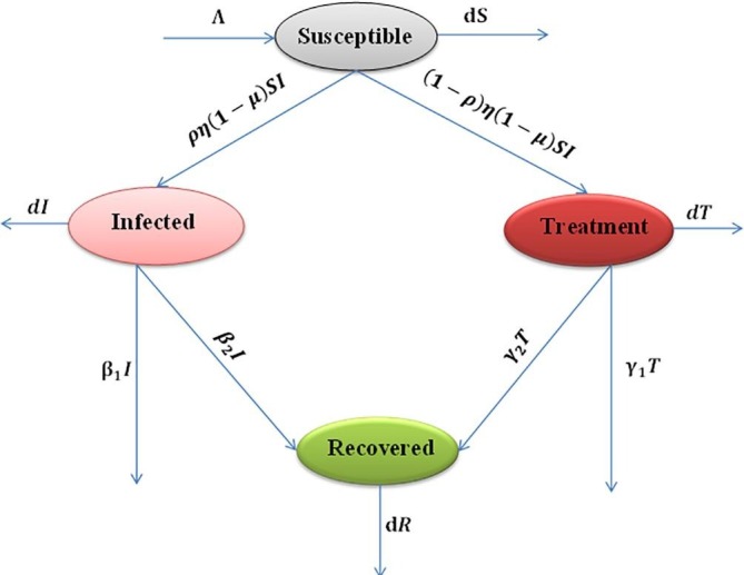
Transfer Diagram of SITR model.

The elasticities for the quantities of interest are

$$\left(E_{\mathrm{\Lambda }}=1\right)$$ (5.16)

$$\left(E_{\eta }=1\right)$$ (5.17)

$$\left(E_{\mu }=-\frac{\mu }{1-\mu }\right)$$ (5.18)

$$\left(E_{\rho }=1\right)$$ (5.19)

$$\left(E_{{\beta }_1}=-\frac{{\beta }_1}{B}\right)$$ (5.20)

$$\left(E_{{\beta }_2}=-\frac{{\beta }_2}{B}\right)$$ (5.21)

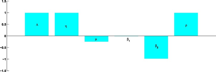
Fig. 2 indicates that, ${\mathcal{R}}_0$ is most sensitive to $\mathrm{\Lambda },\eta ,\rho$ and ${\beta }_2$. The rate $\mu$ has some sensitivity index. It can also be observed that, ${\mathcal{R}}_0$ is less sensitive to ${\beta }_1$, the disease induced death rate.

Fig. 2.

The sensitivity analysis of the basic reproductive number.

The sensitivity indexes for $\mathrm{\Lambda },\eta ,\mu ,\rho ,{\beta }_1$ and ${\beta }_2$, are found to be $1,1,-0.25,1,-0.0164$ and $-0.9833$, respectively, once all parameters are fixed at their baseline values (Fig. 2). Thus, for instance, if the growth rate $\mathrm{\Lambda }$ of susceptible populations is increased or (decreased) by $10\%$, then the value of ${\mathcal{R}}_0$ would increase or (decrease) by $10\%$. Likewise, a $10\%$ increase or (decrease) of the $\eta$ would correspond to a $10\%$ increase or (decrease) of the ${\mathcal{R}}_0,10\%$ increase or (decrease) of $\mu$ would correspond to a $2.5\%$ decrease or (increase) in the value of ${\mathcal{R}}_0,10\%$ increase or (decrease) of the $\rho$ would correspond to a $10\%$ increase or (decrease) of the ${\mathcal{R}}_0$, $10\%$ increase or (decrease) of ${\beta }_1$ would decrease or (increase) the ${\mathcal{R}}_0$ by $0.164\%$ and $10\%$ increase or (decrease) of ${\beta }_2$ would correspond to decrease or (increase) the value of ${\mathcal{R}}_0$ by $9.833\%$.

Therefore, the above interpretations recommend that control strategies that can efficiently decrease the probability of disease transmission $\eta$, growth rate $\mathrm{\Lambda }$ and $\rho$should be used to control the disease transmission effectively. Additionally, increase in the rate of $\mu ,{\beta }_2$ will lead to a decrease in ${\mathcal{R}}_0$. Effect of lockdown $\mu$ on ${\mathcal{R}}_0$ is very small. Since there is no strong evidence to determine those who have been contacted with COVID-19 and those who are not carrying the virus. Due to the situations, preventive measures, such as social and physical distancing, are still the only option to halt the transmission of COVID-19. Since lockdown effect on ${\mathcal{R}}_0$ is very small, so we can avoid this to rescue our economy. (See Table 1 )

Table 1.

Sensitive analysis for India based on sensitive parameters.

x	$\mathrm{\Lambda }$	$\eta$	$\mu$	$\rho$	${\beta }_1$	${\beta }_2$
$E_x$	1	1	$-0.25$	1	$-0.0164$	$-0.9833$

Numerical simulation and discussion

In this section, numerical simulations of the fractional-order epidemiological model (3.4) are conducted to illustrate the theoretical results obtained before. Most non-linear fractional-order differential equations do not have exact analytical solutions and numerical methods are necessary to solve these equations. For the numerical simulation of fractional-order epidemic system, the Adams-Bashforth-Moulton type predictor-corrector scheme is applied. Numerical algorithm for the proposed fractional-order dynamic systems is

$S_{n+1}=S_0+\frac{h^{\alpha }}{\mathrm{\Gamma }(\alpha +2)}\left\{\mathrm{\Lambda }-\eta \left(1-\mu \right)S_{n+1}^p{I}_{n+1}^p-{\mathit{dS}}_{n+1}^p+{\sum }_{j=0}^n{a}_{1,j,n+1}(\mathrm{\Lambda }-\eta \left(1-\mu \right)S_j{I}_j-{\mathit{dS}}_j)\right\}$ $I_{n+1}=I_0+\frac{h^{\alpha }}{\mathrm{\Gamma }(\alpha +2)}\left\{\rho \eta \left(1-\mu \right)S_{n+1}^p{I}_{n+1}^p-{\mathit{BI}}_{n+1}^p+{\sum }_{j=0}^n{a}_{2,j,n+1}(\rho \eta \left(1-\mu \right)S_j{I}_j-{\mathit{BI}}_j)\right\}$ $T_{n+1}=T_0+\frac{h^{\alpha }}{\mathrm{\Gamma }(\alpha +2)}\left\{(1-\rho )\eta \left(1-\mu \right)S_{n+1}^p{I}_{n+1}^p-{\mathit{CT}}_{n+1}^p+{\sum }_{j=0}^n{a}_{2,j,n+1}\left(\right(1-\rho )\eta \left(1-\mu \right)S_j{I}_j-{\mathit{CT}}_j)\right\}$ in which

$\left\{\begin{array}{c}\hfill S_{n+1}^p=S_0+\frac{1}{\mathrm{\Gamma }\left(\alpha \right)}\sum _{j=0}^n{b}_{1,j,n+1}(\mathrm{\Lambda }-\eta \left(1-\mu \right)S_j{I}_j-{\mathit{dS}}_j)\hfill \\ \hfill I_{n+1}^p=I_0+\frac{1}{\mathrm{\Gamma }\left(\alpha \right)}\sum _{j=0}^n{b}_{2,j,n+1}(\rho \eta \left(1-\mu \right)S_j{I}_j-{\mathit{BI}}_j)\hfill \\ \hfill T_{n+1}^p=T_0+\frac{1}{\mathrm{\Gamma }\left(\alpha \right)}\sum _{j=0}^n{b}_{2,j,n+1}\left(\right(1-\rho )\eta \left(1-\mu \right)S_j{I}_j-{\mathit{CT}}_j)\hfill \end{array}\right)$ where$\left\{\begin{array}{c}\hfill b_{1,j,n+1}=\frac{h^{\alpha }}{\alpha }({(n-j+1)}^{\alpha }-{(n-j)}^{\alpha }),0⩽j⩽n\hfill \\ \hfill b_{2,j,n+1}=\frac{h^{\alpha }}{\alpha }({(n-j+1)}^{\alpha }-{(n-j)}^{\alpha }),0⩽j⩽n\hfill \\ \hfill b_{3,j,n+1}=\frac{h^{\alpha }}{\alpha }({(n-j+1)}^{\alpha }-{(n-j)}^{\alpha }),0⩽j⩽n\hfill \end{array}\right)$ $\left\{\begin{array}{c}\hfill a_{1,j,n+1}=\left\{\begin{array}{c}\hfill n^{\alpha +1}-(n-\alpha ){(n+1)}^{\alpha }\hfill \\ \hfill {(n-j+2)}^{\alpha +1}+{(n-j)}^{\alpha +1}-2{(n-j+1)}^{\alpha +1}\hfill \\ \hfill 1\hfill \end{array}\right)\begin{array}{c}\hfill \mathrm{for}j=0\hfill \\ \hfill \mathrm{for}1⩽j⩽n\hfill \\ \hfill \mathrm{for}j=n+1\hfill \end{array}{a}_{2,j,n+1}=\left\{\begin{array}{c}\hfill n^{\alpha +1}-(n-\alpha ){(n+1)}^{\alpha }\hfill \\ \hfill {(n-j+2)}^{\alpha +1}+{(n-j)}^{\alpha +1}-2{(n-j+1)}^{\alpha +1}\hfill \\ \hfill 1\hfill \end{array}\right)\begin{array}{c}\hfill \mathrm{for}j=0\hfill \\ \hfill \mathrm{for}1⩽j⩽n\hfill \\ \hfill \mathrm{for}j=n+1\hfill \end{array}{a}_{3,j,n+1}=\left\{\begin{array}{c}\hfill n^{\alpha +1}-(n-\alpha ){(n+1)}^{\alpha }\hfill \\ \hfill {(n-j+2)}^{\alpha +1}+{(n-j)}^{\alpha +1}-2{(n-j+1)}^{\alpha +1}\hfill \\ \hfill 1\hfill \end{array}\right)\begin{array}{c}\hfill \mathrm{for}j=0\hfill \\ \hfill \mathrm{for}1⩽j⩽n\hfill \\ \hfill \mathrm{for}j=n+1\hfill \end{array}\hfill \end{array}\right)$

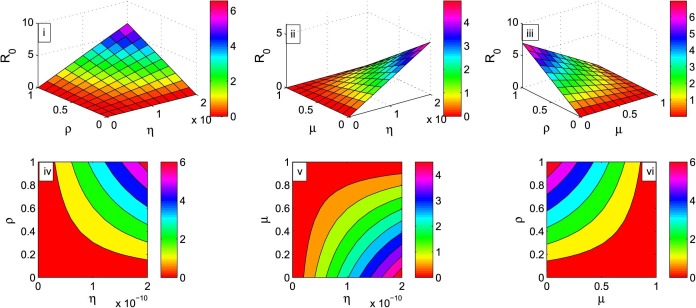
Based on Table 3 , the basic reproduction number is ${\mathcal{R}}_0=3.2776$, which is much greater than 1. Hence the infection spreads so quickly in India. All the figures from Fig. 3 to Fig. 8 are drawn based on the values from Table 2 and Table 3 except the varied parameters. For the proposed model, graphical presentation of ${\mathcal{R}}_0$ with respect to $\eta ,\rho$ and $\mu$ is given in Fig. 3.

Table 3.

Model parameters for COVID-19 system

Parameters	India	Source
$\mathrm{\Lambda }$	$50000$	https://www.mohfw.gov.in/
$\eta$	$0.00000000017$	Estimated
$\rho$	$0.6$	Assumed
${\beta }_1$	$0.001$	Assumed
${\beta }_2$	$0.06$	Assumed
${\gamma }_1$	$0.002$	Estimated
${\gamma }_2$	$0.06$	Estimated
$\mu$	$0.2$	Assumed
d	$0.00002$	https://www.mohfw.gov.in/
$\alpha$	$0.95$	Assumed

Fig. 3.

The figure shows the basic reproduction number ${\mathcal{R}}_0$ when $\left(i\right)$$\eta$ and $\rho$ varies, $\left(\mathit{ii}\right)$$\eta$ and $\mu$ varies, $\left(\mathit{iii}\right)$$\mu$ and $\rho$ varies. Contour plots of basic reproduction number ${\mathcal{R}}_0$ with respect to $\left(\mathit{iv}\right)$$\eta$ and $\rho$, ($v)$$\eta$ and $\mu$, $\left(\mathit{vi}\right)$$\mu$ and $\rho$.

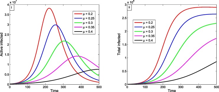
Fig. 8.

(i) Time series of active infected population which is under treatment for different values of $\mu$. (ii) Time series of total infected population which is under Treatment for different values of $\mu$.

Table 2.

Estimated Initial population (as of $1^{\mathit{st}}$July, 2020)

$\mathit{Region}$	$S\left(0\right)$	$I\left(0\right)$	$T\left(0\right)$
$\mathit{India}$	$12\times {10}^8$	$3\times {10}^5$	220114

From Fig. 3(i), we observe that when $\eta$ and $\rho$ gradually decrease, ${\mathcal{R}}_0$ decreases, which means that when infected cases are strictly identified, then ${\mathcal{R}}_0$ gradually decreases, i.e., the rate of spreading of the infection gradually decreases. From Fig. 3(ii), we observe that when $\eta$ gradually increases and $\mu$ gradually decreases, ${\mathcal{R}}_0$ is gradually increased. From Fig. 3(iii), we observe that when $\mu$ gradually increases and $\rho$ gradually decreases, ${\mathcal{R}}_0$ is gradually decreased. In addition,we draw the contour plots for the basic reproduction number ${\mathcal{R}}_0$ with respect to the parameters 3(iv) $\eta$ versus $\rho$, 3(v) $\eta$ versus $\mu$, 3(vi) $\mu$ versus $\rho$ to visualize the influence of the control parameters in controlling the reproduction number ${\mathcal{R}}_0$.

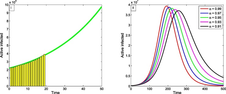
In Fig. 4 (i) the green curve presents infected individuals which are under treatment for this proposed model and bar diagram shows the actual infected individual. Fig. 4(i) depicts the actual infected individual that almost coincides to our proposed model curve from $1^{\mathit{st}}$ July to ${29}^{\mathit{th}}$ July 2020. Therefore, the proposed COVID-19 model is best fitted to the current situation of India.

Fig. 4.

(i) Time series of active infected population from 1/7/2020 to 20/7/2020. (ii) Time series of active infected population which is under treatment for different values of fractional order $\alpha$.

Now taking all the parameters value from Table 2 and Table 3, then if we gradually decreases $\alpha$, then active infected individuals which are under treatment decrease which are presented in Fig. 4(ii).

Fig. 4(ii) shows that, if the fractional order $\alpha$ decreases in long run, then the active infected individuals which are under treatment decrease. From the figure it is clear that when $\alpha =0.99$ then the active infected individuals which are under treatment are nearly $37\times {10}^7$ in around 200 days after that active individuals decrease as day increases and before 500 days it has been vanished. Again, if $\alpha =0.97,\alpha =0.95,\alpha =0.93,\alpha =0.91$ i.e., $\alpha$ decreases and then the number of active cases are decreased and attain the maximum number as days increase. Therefore, the number of active cases are decreased as days increase.

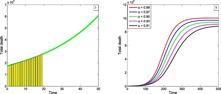
In Fig. 5 (i) the green curve presents total deaths which are under treatment for this proposed model and bar diagram is the actual deaths as per our available data. Fig. 5(i) depicts that the actual deaths almost coincide to our proposed model curve from $1^{\mathit{st}}$ July to ${29}^{\mathit{th}}$ July 2020. Therefore, the proposed COVID-19 model is best fitted to the current situation of India. Here the number of deaths are coming only from treatment section, in infected but not under treatment section. The number of deaths are unknown because of the deaths are not notified in Governmental section from infected zone. So, day by day the number of infected people is increasing and therefore the number of deaths are increased. So, our job has to be identified those people who are infected by COVID-19 and send them to hospital in treatment section such that number deaths may be minimized.

Fig. 5.

(i) Time series of Total deaths from 1/7/2020 to 20/7/2020. (ii) Time series of Total Death case in India for differentent values of fractional order $\alpha$.

Now taking all the parameters value from Table 2 and Table 3, then if we gradually decreases $\alpha$, then the total death of under treatment population decreases, which is presented by Fig. 5(ii).

Fig. 5(ii) shows that if the fractional order $\alpha$ decreases in long run, then the total death cases are decreased and after certain time this rate is stable. From the figure it is clear that when $\alpha =0.99$ then the total death cases are nearly $10\times {10}^8$ in around 400 days after that active individuals are stable as day increases. Again, if $\alpha =0.97,\alpha =0.95,\alpha =0.93,\alpha =0.91$ then the number of total death cases are decreased and attain its maximum number. Therefore the number of total death cases are increased and stable as day increases.

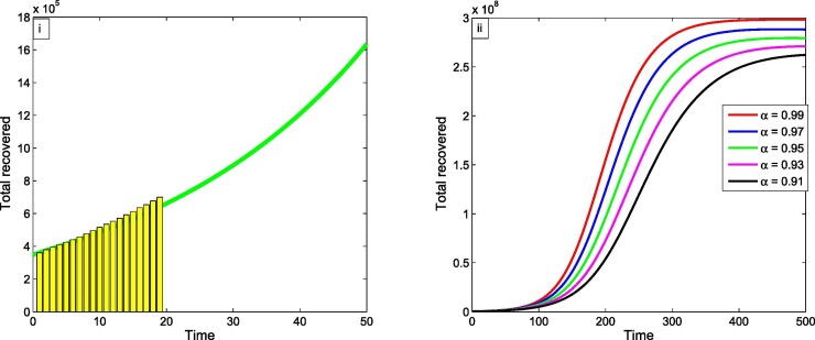
In Fig. 6 (i) the green curve indicates infected individuals which are under treatment for this proposed model and bar diagram refers to the total recoveries as per our available data. Fig. 6(i) depicts that the actual recoveries almost coincide our proposed model curve from $1^{\mathit{st}}$ July to ${29}^{\mathit{th}}$ July 2020. Therefore, the proposed COVID-19 model is best fitted to the current situation of India. Here the number of recoveries are coming only from Treatment section, in infected section the number of recoveries are not notified in Governmental section from infected zone. So they should be increased. This should be a great achievement in our Governmental section in front of whole world. So, the rest of world follows our trend such that infected rate are minimized. So, our job has to be identified those people who are recover from COVID-19 and notify the records.

Fig. 6.

(i) Time series of total recoveries from 1/7/2020 to 20/7/2020. (ii) Time series of active infected population which is under Treatment for different values of fractional order $\alpha$.

Now taking all the parameters value from Table 2 and Table 3. If we gradually decreases $\alpha$ and further steadily decreases of active infected individuals which are under treatment then it is also decreased and is presented by Fig. 6(ii).

Fig. 6(ii) shows that, if the fractional order $\alpha$ decreases in long run, then the total recoveries cases are decreased and after certain time this rate is stable. From the figure it is clear that when $\alpha =0.99$ then the total recoveries cases are nearly $3\times {10}^8$ in around 400 days after that active individuals are stable as day increases. Again, if $\alpha =0.97,\alpha =0.95,\alpha =0.93,\alpha =0.91$ then the number of total recoveries cases are decreased and attain its maximum number as days increase. Therefore, the number of total recoveries cases are increased and stable as day increases.

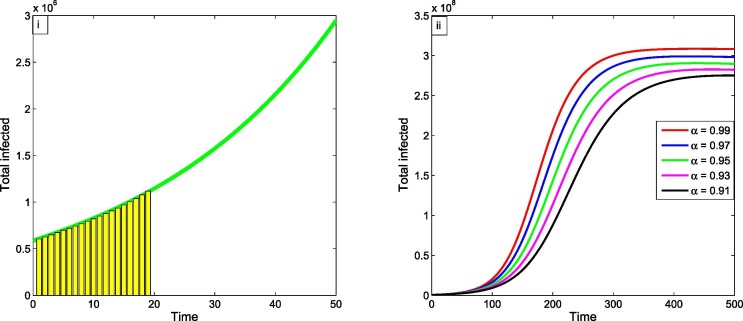
In Fig. 7 (i) the green curve presents infected individual which are under treatment for this proposed model and bar diagram presents the total infected as per our available data. Fig. 7(i) depicts that the total infected almost coincides our proposed model curve from $1^{\mathit{st}}$ July to ${29}^{\mathit{th}}$ July 2020. Therefore, the proposed COVID-19 model is best fitted to the current situation of India. Here the number of total infected are coming only from treatment section, in infected section the number of infected are unknown because the infected ones are not notified in Governmental section from infected zone. So, day by day the number of infected people is increasing due to carefulness of people. So, our job has to be identified those people who are infected by COVID-19 and send them to hospital in treatment section such that number of deaths is are minimized.

Fig. 7.

(i) Time series of total infected from 1/7/2020 to 20/7/2020. (ii) Time series of active infected population which is under treatment for different values of fractional order $\alpha$.

Now taking all the parameters value from Table 2 and Table 3, then if we gradually decreases $\alpha$ and further steadily decreases of active infected individuals which is under treatment it is also decreased and is presented by Fig. 7(ii).

Fig. 7(ii) shows that, if the fractional order $\alpha$ decreases in long run, then the total infected cases are decreased and after certain time this rate is stable. From the figure it is clear that when $\alpha =0.99$ then the total death cases are nearly $3\times {10}^8$ in around 400 days after that active individuals are stable as day increases. Again, if $\alpha =0.97,\alpha =0.95,\alpha =0.93,\alpha =0.91$ then the number of total death cases is decreased and attain its maximum number as days increase. Therefore, the number of total death cases is increased and stable as day increases.

From, Fig. 8(i), we observe that when $\mu$ is considered as a lockdown effect, then an increases in the rate of lockdown effect the number of active infected cases is minimized. If $\mu =0.2$ i.e. 20% of lockdown implies that the high number of active infected cases reaches to 225 day’s but the percentage of lockdown effect increases and then the number of active infected cases is minimized and takes some more extra days.

Fig. 8(ii) shows that if the lockdown effect $\mu$ increases in long run, then the total infected cases is decreased and after certain time this rate is stable. Clearly, the rate at which infected cases are slow is due to increasing of lockdown percentage. From the figure it is clear that when $\alpha =0.99$ then the total infected cases are nearly $29\times {10}^7$ in around 400 days after that active individuals are stable as day increases. Again, if $\alpha =0.97,\alpha =0.95,\alpha =0.93,\alpha =0.91$ then the number of total infected cases is decreased and attain its maximum number as days increase and then the number of total infected cases is increased and stable as day increases.

Our main aim is to minimize the infection and death rate due to COVID-19. To control such cases we should identify the infected case and gives better treatment. We identify the infected individuals so that spread of infection should be minimized. Finally, In this paper, we extend the classical SIR model with treatment factor to a system of fractional ordinary differential equations (FODEs). For our fractional-order model, we determine the basic reproduction ${\mathcal{R}}_0$ and prove that if ${\mathcal{R}}_0<1$, the disease-free equilibrium is locally asymptotically stable. We establish the existence conditions of endemic equilibrium points. We prove the global stability of disease free equilibrium point and endemic equilibrium point. From sensitivity analysis of basic reproduction number ${\mathcal{R}}_0$ it shows that if we identify the rate of infection from susceptible zone to infected zone and give better treatment then the deaths rate may be minimized and people who are infected too. The stability of endemic equilibrium points can be controlled by modifying the value of $\alpha$. In fact, the fractional-order model can be achieved in the steady state by controlling the parameters which affect the value of $\alpha$ as shown in the Fig. 4(ii), Fig. 5(ii), Fig. 6(ii) and Fig. 7(ii). In the end of our paper, the analytical results are confirmed by some numerical simulations for real data related to COVID-19 disease. In Fig. 8, it is shown that the deadly disease can be controlled by restriction of appropriate percentage of lockdown. From this model we can easily identify the number of percussion that is required to avoid the infection from COVID-19. The proposed model can provide useful information for understanding and prediction of the transmission of different epidemics worldwide. Most importantly, the goal of this model is to estimate in future the number of total infected, active cases, deaths as well as the recoveries from COVID-19. This helps to decide the future decision so that we control or minimize the above cases.

Future Expectation for the model system:

From the above obtained results we can conclude that if we have not be able to control the infected rate then the deaths rate is unstoppable. From this paper we expect the future of infected individuals from Fig. 4(i). We discuss that in the following table:

From the Table 4 it is clear that if we could not control the spread of COVID-19 in human body then day by day active infected cases are rapidly increasing.

Table 4.

Expected number of future prediction.

Date	Total Infected	Total death
01/08/2020	$1.673\times {10}^6$	$3.773\times {10}^4$
01/09/2020	$4.253\times {10}^6$	$8.543\times {10}^4$
01/10/2020	$1.017\times {10}^7$	$1.959\times {10}^5$
01/11/2020	$2.403\times {10}^7$	$4.62\times {10}^5$
01/12/2020	$5.137\times {10}^7$	$1.019\times {10}^6$

CRediT authorship contribution statement

S.S. Askar: Formal analysis, Funding acquisition, Investigation, Methodology, Project administration, Resources, Software, Supervision, Validation, Visualization, Writing - review & editing. Dipankar Ghosh: Conceptualization, Data curation, Formal analysis, Investigation, Methodology, Project administration, Resources, Validation, Visualization, Writing - original draft. P.K. Santra: Conceptualization, Data curation, Formal analysis, Project administration, Resources, Software, Supervision, Validation, Visualization, Writing - original draft. Abdelalim A. Elsadany: Conceptualization, Data curation, Formal analysis, Investigation, Methodology, Visualization, Writing - original draft, Writing - review & editing. G.S. Mahapatra: Conceptualization, Data curation, Formal analysis, Funding acquisition, Investigation, Methodology, Project administration, Software, Supervision, Validation, Visualization, Writing - original draft, Writing - review & editing.

Declaration of Competing Interest

The authors declare that they have no known competing financial interests or personal relationships that could have appeared to influence the work reported in this paper.

References

- 1.Podlubny I. Academic Press; California, USA: 1999. Fractional differential equations. [Google Scholar]
- 2.Samko S.G., Kilbas A.A., Marichev O.I. CRC; 1993. Fractional integrals and derivatives: theory and applications. [Google Scholar]
- 3.Li H.L., Zhang L., Hu C., Jiang Y.L., Teng Z. Dynamical analysis of a fractional-order predator-prey model incorporating a prey refuge. J Appl Math Comput. 2017;54:435–449. [Google Scholar]
- 4.Saleh W. Kílíçman A. Note on the fractional mittag-leffler functions by applying the modified riemann-liouville derivatives. Bol Soc Parana Mat; 2019.
- 5.Delavari H., Baleanu D., Sadati J. Stability analysis of Caputo fractional-order nonlinear systems revisited. Nonlinear Dyn. 2012;67:2433–2439. [Google Scholar]
- 6.Leon C.V.D. Volterra-type Lyapunov functions for fractional-order epidemic systems. Commun Nonlinear Sci Numer Simul. 2015;24:75–85. [Google Scholar]
- 7.Diethelm K., Ford N., Freed A. A predictor–corrector approach for the numerical solution of fractional differential equations. Nonlinear Dyn. 2002;29:3–22. [Google Scholar]
- 8.Diethelm K. Springer; Berlin: 2010. The analysis of fractional differential equations. [Google Scholar]
- 9.Hong-Li L., Long Z., Cheng H., Yao-Lin J., Zhidong T. Dynamical analysis of a fractional-order predator-prey model incorporating a prey refuge. J Appl Math Comput. 2016;54:435–449. [Google Scholar]
- 10.Choi S.K., Kang B., Koo N. Stability for Caputo fractional differential systems. Abstr Appl Anal. 2014;2014:1–6. [Google Scholar]
- 11.Boukhouima A., Hattaf K., Yousfi N. Dynamics of a fractional order HIV infection model with specific functional response and cure rate. Int J Differ Equ. 2017 doi: 10.1155/2017/8372140. [DOI] [Google Scholar]
- 12.Chen M., Clemence D.P. Analysis of and numerical schemes for a mouse population model in Hantavirus epidemics. J Differ Equ Appl. 2006;12:887–899. [Google Scholar]
- 13.Van den Driessche P., Watmough J. Reproduction numbers and sub-threshold endemic equilibria for compartmental models of disease transmission. Math Biosci. 2002;180:29–48. doi: 10.1016/s0025-5564(02)00108-6. [DOI] [PubMed] [Google Scholar]
- 14.Ahmed E., El-Sayed A., El-Saka H.A. Equilibrium points, stability and numerical solutions of fractional-order predator–prey and rabies models. J Math Anal Appl. 2007;325:542–553. [Google Scholar]
- 15.Matignon D. vol. 2. Lille; France: 1996. Stability results for fractional differential equations with applications to control processing; pp. 963–968. (Computational engineering in systems applications). [Google Scholar]
- 16.Chitnis N., Hyman J.M., Cushing J.M. Determining important parameters in the spread of malaria through the sensitivity analysis of a mathematical model. Bull Math Biol. 2008;70:1272–1296. doi: 10.1007/s11538-008-9299-0. [DOI] [PubMed] [Google Scholar]
- 17.Teodoro G.S., Machado J.T., de Oliveira E.C. A review of definitions of fractional derivatives and other operators. J Comput Phys. 2019;388:195–208. [Google Scholar]
- 18.Du M., Wang Z., Hu H. Measuring memory with the order of fractional derivative. Sci Rep. 2013;3:3431. doi: 10.1038/srep03431. [DOI] [PMC free article] [PubMed] [Google Scholar]
- 19.Postavaru O., Anton S.R., Toma A. COVID-19 pandemic and chaos theory. Math Comput Simul. 2021;181:138–149. doi: 10.1016/j.matcom.2020.09.029. [DOI] [PMC free article] [PubMed] [Google Scholar]
- 20.Zhang Z, Zeb A, Egbelowo OF, Erturk VS. Dynamics of a fractional order mathematical model for COVID-19 epidemic. Adv Diff Equ 2020(1), art. no. 420. [DOI] [PMC free article] [PubMed]
- 21.Rezapour S, Mohammadi H, Samei ME. SEIR (2020) epidemic model for COVID-19 transmission by Caputo derivative of fractional order. Adv Diff Equ 2020 (1), art. no. 490. [DOI] [PMC free article] [PubMed]
- 22.Ahmed I, Baba IA, Yusuf A, Kumam P, Kumam W. Analysis of Caputo fractional-order model for COVID-19 with lockdown. Adv Diff Equ 2020 (1), art. no. 394. [DOI] [PMC free article] [PubMed]
- 23.Shaikh AS, Shaikh IN, Nisar KS. A mathematical model of COVID-19 using fractional derivative: outbreak in India with dynamics of transmission and control. Adv Diff Equ (1); 2020, art. no. 373. [DOI] [PMC free article] [PubMed]
- 24.Ahmad S, Ullah A, Shah K, Salahshour S, Ahmadian A, Ciano T. Fuzzy fractional-order model of the novel coronavirus. Adv Diff Equ 2020 (1), art. no. 472. [DOI] [PMC free article] [PubMed]
- 25.Baleanu D, Mohammadi H, Rezapour S. A fractional differential equation model for the COVID-19 transmission by using the Caputo-Fabrizio derivative. Adv Diff Equ 2020 (1), art. no. 299. [DOI] [PMC free article] [PubMed]
- 26.Khan MA, Atangana A, Alzahrani E, Fatmawati. The dynamics of COVID-19 with quasrantined and isolation. Adv Diff Equ 1; 2020, art. no. 425. [DOI] [PMC free article] [PubMed]
- 27.Bushnaq S, Shah K, Alrabaiah H. On modeling of coronavirus-19 disease under Mittag-Leffler power law. Adv Diff Equ (1); 2020, art. no. 487. [DOI] [PMC free article] [PubMed]
- 28.Yadav RP, Renu Verma. A numerical simulation of fractional order mathematical modeling of COVID-19 disease in case of Wuhan China. Chaos Solitons Fractals 140; 2020, art. no. 110124. [DOI] [PMC free article] [PubMed]
- 29.Rahman MU, Arfan M, Shah K, Gó mez-Aguilar JF. Investigating a nonlinear dynamical model of COVID-19 disease under fuzzy caputo, random and ABC fractional order derivative. Chaos Solitons Fractals 140; 2020, art. no. 110232. [DOI] [PMC free article] [PubMed]
- 30.Mohammad M, Trounev A. On the dynamical modeling of COVID-19 involving Atangana-Baleanu fractional derivative and based on Daubechies framelet simulations. Chaos Solitons Fractals 140; 2020, art. no. 110171. [DOI] [PMC free article] [PubMed]
- 31.Tuan NH, Mohammadi H, Rezapour S. A mathematical model for COVID-19 transmission by using the Caputo fractional derivative. Chaos Solitons Fractals 140; 2020, art. no. 110107. [DOI] [PMC free article] [PubMed]
- 32.Khan M., Atangana A. Modeling the dynamics of novel coronavirus (2019-nCov) with fractional derivative. Alexandria Eng J. 2020 [Google Scholar]
- 33.Ahmad S, Ullah A, Al-Mdallal QM, Khan H, Shah K, Khan. A Fractional order mathematical modeling of COVID-19 transmission. Chaos Solitons Fractals 139; 2020, art. no. 110256. [DOI] [PMC free article] [PubMed]
- 34.Shah K., Khan Z.A., Ali A., Amin R., Khan H., Khan A. Haar wavelet collocation approach for the solution of fractional order COVID-19 model using Caputo derivative. Alexandria Eng J. 2020;59(5):3221–3231. [Google Scholar]
- 35.Sher M., Shah K., Khan Z.A., Khan H. A Computational and theoretical modeling of the transmission dynamics of novel COVID-19 under Mittag-Leffler Power Law. Alexandria Eng J. 2020;59(5):3133–3147. [Google Scholar]
- 36.Higazy M. Novel (2020) fractional order SIDARTHE mathematical model of COVID-19 pandemic. Chaos Solitons Fractals 138, art. no. 110007. [DOI] [PMC free article] [PubMed]
- 37.Alkahtani BST, Alzaid SS. A novel mathematics model of covid-19 with fractional derivative. Stability and numerical analysis. Chaos Solitons Fractals 138; 2020, art. no. 110006. [DOI] [PMC free article] [PubMed]
- 38.Zhang Y, Yu X, Sun H, Tick GR, Wei W, Jin B. Applicability of time fractional derivative models for simulating the dynamics and mitigation scenarios of COVID-19. Chaos Solitons Fractals 138; 2020, art. no. 109959. [DOI] [PMC free article] [PubMed]
- 39.Xu C., Yu Y., Chen Y.Q., Lu Z. Forecast analysis of the epidemics trend of COVID-19 in the USA by a generalized fractional-order SEIR model. Nonlinear Dyn. 2020;101(3):1621–1634. doi: 10.1007/s11071-020-05946-3. [DOI] [PMC free article] [PubMed] [Google Scholar]
- 40.Lu Z., Yu Y., Chen Y.Q., Ren G., Xu C., Wang S., Yin Z. A fractional-order SEIHDR model for COVID-19 with inter-city networked coupling effects. Nonlinear Dyn. 2020;101(3):1717–1730. doi: 10.1007/s11071-020-05848-4. [DOI] [PMC free article] [PubMed] [Google Scholar]
- 41.Rajagopal K., Hasanzadeh N., Parastesh F., Hamarash I.I., Jafari S., Hussain I. A fractional-order model for the novel coronavirus (COVID-19) outbreak. Nonlinear Dyn. 2020;101(1):711–718. doi: 10.1007/s11071-020-05757-6. [DOI] [PMC free article] [PubMed] [Google Scholar]
- 42.Shah K, Abdeljawad T, Mahariq I, Jarad F, Deniz S. Qualitative analysis of a mathematical model in the time of COVID-19. BioMed Res Int 2020, art. no. 5098598. [DOI] [PMC free article] [PubMed]
- 43.Arfan M., Shah K., Abdeljawad T., Mlaiki N., Ullah A. A Caputo power law model predicting the spread of the COVID-19 outbreak in Pakistan. Alexandria Eng J. 2020 [Google Scholar]
- 44.Alrabaiah H., Arfan M., Shah K., Mahariq I., Ullah A. A comparative study of spreading of novel corona virus disease by ussing fractional order modified SEIR model. Alexandria Eng J. 2020 [Google Scholar]
- 45.Owoyemi A.E., Sulaiman I.M., Mamat M., Olowo S.E., Adebiyi O.A., Zakaria Z.A. Analytic numeric solution of coronavirus (Covid-19) pandemic model in fractional-order. Commun Math Biol Neurosci. 2020:1–18. art. no. 61. [Google Scholar]
- 46.Abdullahi Baba I., Ahmad Nasidi B. Fractional order epidemic model for the dynamics of novel COVID-19. Alexandria Eng J. 2020 [Google Scholar]
- 47.Higazy M., Alyami M.A. New Caputo-Fabrizio fractional order SEIASqEqHR model for COVID-19 epidemic transmission with genetic algorithm based control strategy. Alexandria Eng J. 2020 [Google Scholar]
- 48.Abbas M.I., Ragusa M.A. Solvability of Langevin equations with two Hadamard fractional derivatives via Mittag-Leffler functions. Appl Anal. 2021 doi: 10.1080/00036811.2020.1839645. [DOI] [Google Scholar]
- 49.Rahman A.G., Shah K. Mathematical analysis of implicit impulsive switched coupled evolution equations. Results Math. 2021;74:142. doi: 10.1007/s00025-019-1066-z. [DOI] [Google Scholar]
- 50.Rahman A.G., Ahmed S., Haq F. Application of topological degree method in quantitative behavior of fractional differential equations. Filomat. 2020;34(2):421–432. doi: 10.2298/FIL2002421R. [DOI] [Google Scholar]