A latent unknown clustering integrating multi-omics data (LUCID) with phenotypic traits

Abstract

Motivation

Epidemiologic, clinical and translational studies are increasingly generating multiplatform omics data. Methods that can integrate across multiple high-dimensional data types while accounting for differential patterns are critical for uncovering novel associations and underlying relevant subgroups.

Results

We propose an integrative model to estimate latent unknown clusters (LUCID) aiming to both distinguish unique genomic, exposure and informative biomarkers/omic effects while jointly estimating subgroups relevant to the outcome of interest. Simulation studies indicate that we can obtain consistent estimates reflective of the true simulated values, accurately estimate subgroups and recapitulate subgroup-specific effects. We also demonstrate the use of the integrated model for future prediction of risk subgroups and phenotypes. We apply this approach to two real data applications to highlight the integration of genomic, exposure and metabolomic data.

Availability and Implementation

The LUCID method is implemented through the LUCIDus R package available on CRAN (https://CRAN.R-project.org/package=LUCIDus).

Supplementary information

Supplementary materials are available at Bioinformatics online.

1 Introduction

Advancements in technology have made multi-omics data acquisition accessible for researchers and practitioners. The availability of such data, including genomic data, somatic profiles, metabolite measurements, proteomics information, etc., has facilitated new insights into the underlying etiologic mechanism of disease (Curtis et al., 2012). Despite the great potential, multi-omics data have many analytic challenges including integration of differing sources of multi-omics data, the large dimensions of the data and harmonization of various underlying biological hypotheses.

Potential solutions include conventional techniques, such as principal components or factor analysis aimed at estimating clusters of individuals or variable selection algorithms (e.g. lasso) to identify factors (Wu et al., 2019). However, for these approaches it is often unclear how to interpret or combine multiple types of omics data or how to select features from the high-dimensional data. To handle such situations, Shen et al. proposed a method called iCluster for integrative clustering using multiple types of omics data via a joint Gaussian latent variable model with regularization techniques (Mo et al., 2013; Shen et al., 2009). Other integrative methods have been guided by specific hypotheses within the framework of mediation modeling (Huang et al., 2014, 2015). These approaches attempt to explore direct and indirect effects of various features, but across multiple data types of high dimension, interpretation can be challenging. Finally, investigators can focus on omic-specific analyses to infer relationships that potentially can guide biology. Such analyses include pathway analysis with gene expression through the use of ingenuity pathway analysis (QIAGEN Inc., https://www.qiagenbioinformatics.com/products/ingenuitypathway-analysis). Another example for metabolomic analyses includes mummichog (Li et al., 2013), an approach focused on estimating functional activity and pathway relationships without formal identification of the individual untargeted metabolites.

Here, we present a novel approach, latent unknown clustering with integrated data (LUCID), to perform integrative analyses using multi-omics data with phenotypic traits, leveraging their underlying causal relationships in latent cluster estimations. A directed acyclic graph (DAG) is used to illustrate the underlying biological relevance of different components from integrated data in our method. A joint probabilistic model with a latent variable for clustering integrates data in the DAG. Unlike other clustering and data reduction methods, the latent variable links various sources of multi-omics data explicitly to the outcome of interest. An expectation–maximization (EM) algorithm is used to obtain likelihood-based estimates of the latent cluster assignments and model parameters simultaneously (Little and Rubin, 2002). Regularization paths are followed to accommodate settings with high-dimensional data (Tibshirani, 1996). We evaluate the performance of our approach using extensive simulations and with comparison to alternative approaches (e.g. iCluster and lasso). Finally, we apply our method to genetic, exposure, metabolomic and outcome data from two applied studies (Goran et al., 2004; Haile et al., 1999).

2 Materials and methods

2.1 LUCID latent clustering mode

Figure 1 presents a DAG for the integrated analysis. Here, $\mathbf{G}$ is an genetic/exposure data matrix of dimension $n\times p$ with columns being potentially determinant features, such as germline genetic factors or long-term environmental exposures and rows being samples, $X$ is a categorical latent clustering variable for each subject with K levels, $\mathbf{Z}$ is a $n\times m$-dimensional matrix of standardized continuous biomarkers for the same samples and $\mathrm{Y}$ is an n-dimensional vector of the phenotypic trait. Circled variables in the DAG are model parameters. This DAG implies a conditional independence among $X$ given $\mathbf{G}$, $\mathbf{Z}$ given $X$ and $Y$ given $X$.

Fig. 1.

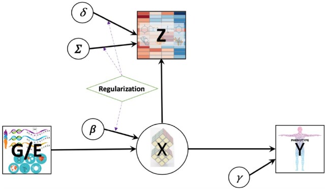
Joint model integrating genetic/environmental features, metabolite and phenotypic traits. Square versus circle: observed data versus latent clusters or unobserved model parameters; diamond: the penalty term for regularization, e.g. lasso

Let $f\left(X\right|\mathbf{G};\mathit{\beta })$, $f\left(\mathbf{Z}\right|X;\mathit{\delta },\mathbf{\Sigma })$ and $f\left(Y\right|X;\mathit{\gamma })$ denote the probability mass functions (PMF) for discrete random variables or the probability density functions (PDF) for continuous random variables. Then, the observed log-likelihood based on the joint distribution of $\mathbf{Z}$ and $Y$ conditioning on $\mathbf{G}$ is:

$$\begin{array}{c}l(\mathbf{\Theta })=\sum _{\mathit{i}=1}^{\mathit{n}}\hspace{0.17em}\text{log}\hspace{0.17em}f({\mathit{Z}}_i,Y_i|{\mathbf{G}}_{\mathrm{i}};\mathit{\beta },\mathit{\delta },\mathbf{\Sigma },\mathit{\gamma })\hfill \\ =\sum _{\mathit{i}=1}^{\mathit{n}}\hspace{0.17em}\text{log}\hspace{0.17em}\sum _{j=1}^{k}f({\mathit{Z}}_i,Y_i,X_i=j|{\mathbf{G}}_{\mathrm{i}};\mathit{\beta },\mathit{\delta },\mathbf{\Sigma },\mathit{\gamma })\\ =\sum _{\mathit{i}=1}^{\mathit{n}}\hspace{0.17em}\text{log}\hspace{0.17em}\sum _{j=1}^{k}f(X_i|{\mathbf{G}}_{\mathrm{i}};\mathit{\beta })f({\mathit{Z}}_i|X_i;\mathit{\delta },\mathbf{\Sigma })f(Y_i|X_i;\mathit{\gamma })\end{array}$$ (1)

where $\mathbf{\Theta }$ is a generic notation standing for all model parameters, including $\mathit{\beta }$, $\mathit{\delta }$, $\mathbf{\Sigma }$ and $\mathit{\gamma }$.

We assume X has k categories and follows a multinomial distribution conditioning on G, Z follows a multivariate normal distribution conditioning on X, and Y follows a normal distribution conditioning on X. See Supplementary Material S1 for Y as a binary outcome. Additionally, if we denote $S(·)$ to be a sigmoid or softmax function, $\varphi (·)$ to be the PDF for a normal random variable. Then, the log-likelihood of model parameters becomes:

$$\begin{array}{c}l(\mathbf{\Theta })=\sum _{\mathit{i}=1}^{\mathit{n}}\hspace{0.17em}\text{log}\hspace{0.17em}\sum _{j=1}^{k}f(X_i|{\mathbf{G}}_{\mathrm{i}};\mathit{\beta })f({\mathit{Z}}_i|X_i;\mathit{\delta },\mathbf{\Sigma })f(Y_i|X_i;\mathit{\gamma })\hfill \\ =\sum _{\mathit{i}=1}^{\mathit{n}}\hspace{0.17em}\text{log}\hspace{0.17em}\sum _{j=1}^{k}S(\beta ,j,{\mathbf{G}}_{\mathrm{i}})\varphi ({\mathbf{Z}}_i;{\delta }_j,{\Sigma }_j)\varphi (Y_i;{\gamma }_j,{\sigma }_j)\end{array}$$ (2)

2.2 Joint estimating through latent cluster via EM algorithm

We further define the posterior probability of belonging to latent cluster j given observed data and parameter values as $P(X_i=j|\mathcal{D};\mathbf{\Theta })$. The parameters of interest include the posterior probability of latent cluster membership, genetic effect $\mathit{\beta }$ (the log odds ratio of cluster inclusion for each corresponding factor G or E), cluster-specific bio-feature means $\mathit{\delta }$ (the mean difference in each biomarker Z for each cluster) and covariance matrices $\mathrm{\Sigma }$, and mean effect of the outcome $\mathit{\gamma }$ (the mean difference in the outcome Y for each cluster for a continuous outcome and the log odds ratio for each cluster for a binary outcome). To obtain maximum-likelihood estimates (MLE) of model parameters, we maximize the expectation of complete data log-likelihood. Detailed derivations are presented in Supplementary Material S2. Specifically, the expectation of complete data log-likelihood for the DAG model is:

$$\begin{array}{c}Q\left(\mathbf{\Theta }\right)=\sum _{i=1}^n\sum _{j=1}^{k}P\left(X_i=j|\mathcal{D};\mathbf{\Theta }\right)\text{log}\hspace{0.17em}\frac{S\left(\beta ,j,{\mathbf{G}}_{\mathrm{i}}\right)}{P\left(X_i=j|\mathcal{D};\mathbf{\Theta }\right)}\\ +\sum _{i=1}^n\sum _{j=1}^{k}P\left(X_i=j|\mathcal{D};\mathbf{\Theta }\right)\text{log}\hspace{0.17em}\frac{\varphi \left({\mathbf{Z}}_i;{\delta }_j,{\Sigma }_j\right)}{P\left(X_i=j|\mathcal{D};\mathbf{\Theta }\right)}\\ +\sum _{i=1}^n\sum _{j=1}^{k}P\left(X_i=j|\mathcal{D};\mathbf{\Theta }\right)\text{log}\hspace{0.17em}\frac{\varphi \left(Y_i;{\gamma }_j,{\sigma }_j\right)}{P(X_i=j|\mathcal{D};\mathbf{\Theta })}\end{array}$$ (3)

The EM algorithm is applied to handle optimization and estimate model parameters. We first define the responsibility ($r$) as the conditional probability of being in latent cluster j given observed data and current values of parameter estimates at iteration t, which is:

$$\begin{array}{c}{r}_{\mathit{ij}}=P\left(X_i=j|\mathcal{D};{\mathbf{\Theta }}^{\left(t\right)}\right)=P\left(X_i=j|{\mathbf{G}}_i,{\mathbf{Z}}_i,Y_i;{\mathbf{\Theta }}^{\left(t\right)}\right)\hfill \\ =\frac{f\left(X_i=j|{\mathbf{G}}_{\mathrm{i}};{\mathbf{\Theta }}^{\left(t\right)}\right)f\left({\mathit{Z}}_i|X_i=j;{\mathbf{\Theta }}^{\left(t\right)}\right)f\left(Y_i|X_i=j;{\mathbf{\Theta }}^{\left(t\right)}\right)}{{\sum }_{j}f\left(X_i=j|{\mathbf{G}}_{\mathrm{i}};{\mathbf{\Theta }}^{\left(t\right)}\right)f\left({\mathit{Z}}_i|X_i=j;{\mathbf{\Theta }}^{\left(t\right)}\right)f\left(Y_i|X_i=j;{\mathbf{\Theta }}^{\left(t\right)}\right)}\end{array}$$ (4)

In the E-step, we compute the expectation of complete data log-likelihood $Q\left(\mathbf{\Theta }\right)$ by using responsibilities as imputed values for posterior probabilities of latent clusters. Thus, substituting $P\left(X_i=j||\mathcal{D};\mathbf{\Theta }\right)$ with $r_{\mathit{ij}}$ in (3), we now have:

$$\begin{array}{c}Q\left(\mathbf{\Theta }\right)=\sum _{i=1}^n\sum _{j=1}^k{r}_{\mathit{ij}}\hspace{0.17em}\text{log}\hspace{0.17em}\frac{S\left(\beta ,j,{\mathbf{G}}_{\mathrm{i}}\right)}{r_{\mathit{ij}}}+\sum _{i=1}^n\sum _{j=1}^k{r}_{\mathit{ij}}\hspace{0.17em}\text{log}\hspace{0.17em}\frac{\varphi \left({\mathbf{Z}}_i;{\delta }_j,{\Sigma }_j\right)}{r_{\mathit{ij}}}\hfill \\ +\sum _{i=1}^n\sum _{j=1}^k{r}_{\mathit{ij}}\hspace{0.17em}\text{log}\hspace{0.17em}\frac{\varphi \left(Y_i;{\gamma }_j,{\sigma }_j\right)}{r_{\mathit{ij}}}=\sum _{i=1}^n\sum _{j=1}^k{r}_{\mathit{ij}}\hspace{0.17em}\text{log}\hspace{0.17em}S\left(\beta ,j,{\mathbf{G}}_{\mathrm{i}}\right)\\ -\frac{1}{2}\sum _{i=1}^n\sum _{j=1}^k{r}_{\mathit{ij}}{\left({\mathbf{Z}}_{\mathbf{i}}-{\mathit{\delta }}_j\right)}^T{\Sigma }_j^{-1}\left({\mathbf{Z}}_{\mathbf{i}}-{\mathit{\delta }}_j\right)-\frac{1}{2}\sum _{i=1}^n\sum _{j=1}^k{r}_{\mathit{ij}}\hspace{0.17em}\text{log}\hspace{0.17em}\left|{\Sigma }_j\right|\\ -\frac{1}{2}\sum _{i=1}^n\sum _{j=1}^k\frac{r_{\mathit{ij}}{\left(Y_i-{\mu }_j\right)}^2}{{\sigma }_j^2}-\frac{1}{2}\sum _{i=1}^n\sum _{j=1}^k{r}_{\mathit{ij}}\hspace{0.17em}\text{log}\hspace{0.17em}{\sigma }_j^2-3\sum _{i=1}^n\sum _{j=1}^k{r}_{\mathit{ij}}\hspace{0.17em}\text{log}\hspace{0.17em}{r}_{\mathit{ij}}\end{array}$$ (5)

The M-step is then to update parameter estimates by maximizing (5) computed in the current E-step. This results in the following estimates of $\mathit{\beta }$, $\mathit{\delta }$, $\mathrm{\Sigma }$, $\mathit{\gamma }$ and $\mathit{\sigma }$ at iteration t + 1:

$${\mathit{\beta }}^{(t+1)}=\mathit{argma}{x}_{\mathit{\beta }}\sum _{i=1}^n\sum _{j=1}^k{r}_{\mathit{ij}}\log S\left(\mathit{\beta },j,{\mathbf{G}}_{\mathrm{i}}\right)$$ (6)

$${\mathit{\delta }}_j^{(t+1)}=\frac{{\sum }_{i=1}^n{r}_{\mathit{ij}}{\mathbf{Z}}_{\mathrm{i}}}{{\sum }_{i=1}^n{r}_{\mathit{ij}}}\mathrm{ }$$ (7)

$${\mathrm{\Sigma }}_j^{(t+1)}=\frac{{\sum }_{i=1}^n{r}_{\mathit{ij}}({\mathbf{Z}}_{\mathrm{i}}-{\mathit{\delta }}_j^{(t+1)}){({\mathbf{Z}}_{\mathrm{i}}-{\mathit{\delta }}_j^{(t+1)})}^T}{{\sum }_{i=1}^n{r}_{\mathit{ij}}}\mathrm{ }$$ (8)

$${\mathit{\mu }}_j^{(t+1)}=\frac{{\sum }_{i=1}^n{r}_{\mathit{ij}}{\mathrm{Y}}_i}{{\sum }_{i=1}^n{r}_{\mathit{ij}}}\mathrm{ }$$ (9)

$${\mathit{\sigma }}_j^{(t+1)}=\sqrt{\frac{{\sum }_{i=1}^n{r}_{\mathit{ij}}{\left(Y_i-{\mu }_j^{(t+1)}\right)}^2}{{\sum }_{i=1}^n{r}_{\mathit{ij}}}}\mathrm{ }$$ (10)

Although the maximization in (6) does not have a closed-form solution, it can be easily solved iteratively since it is a convex optimization problem (Venables and Ripley, 2002). Likewise, parameters in (9, 10) could be estimated through maximizing the log-likelihood of linear regression predicting a continuous outcome with posterior probabilities of latent clusters. By doing this, we postulate equal variance (σ) among the outcome of interest across different latent clusters due to the homoscedasticity assumption of linear regression. Specifically, when fitting $Y={\mu }_1{r}_1+{\mu }_2{r}_2+\cdots +{\mu }_k{r}_k+\epsilon ={\mathit{\mu }}^{\mathit{T}}\mathbf{r}+\epsilon$,

$${\widehat{\mathit{\gamma }}}^{(t+1)}={\widehat{\mathit{\mu }}}_{\mathit{OLS}}^{(t+1)}$$ (11)

$${\widehat{\mathit{\sigma }}}^{(t+1)}=\mathrm{ }\mathit{SD}\left(\widehat{\epsilon }\right)=\mathit{SD}(Y-{\widehat{\mathit{\mu }}}^{\mathit{T}}\mathbf{r})$$ (12)

As the number of latent clusters (K) needs to be pre-specified for LUCID, we recommend selecting an optimal K using the Bayesian information criterion (BIC) by fitting the model over a range of pre-specified values for K. The optimal K can be subsequently identified by the candidate model with the minimum BIC.

2.3 Sparse solutions for high-dimensional multi-omics features

In the case of high-dimensional $\mathbf{G}$ and $\mathbf{Z}$, sparse solutions of $\mathit{\beta }$, $\mathit{\delta }$ and $\mathrm{\Sigma }$ are obtained via a lasso-type penalty (Hastie et al., 2009; Murphy, 2012; Tibshirani, 1996). For ${\mathit{\beta }}_{\mathit{LASSO}}$:

$${\mathit{\beta }}_{\mathit{LASSO}}^{\left(t+1\right)}=\mathit{argma}{x}_{\mathit{\beta }}\mathrm{ }\{{\sum }_{i=1}^n{\sum }_{j=1}^k{r}_{\mathit{ij}}\log S\left(\mathit{\beta },j,{\mathbf{G}}_{\mathrm{i}}\right)-{\rho }_G{\sum }_{l=1}^{p+1}{\sum }_{j=1}^k\left|{\beta }_{\mathit{lj}}\right|\}\mathrm{ }$$ (13)

To obtain sparse estimates of $\mathit{\delta }$ and $\mathbf{\Sigma }$, we implement the lasso-type scout approach (Witten and Tibshirani, 2009). $\mathbf{\Sigma }$ is first updated by the following maximization while penalizing the $L_1$ norm of its inverse:

$${\left({\mathbf{\Sigma }}_j^{(t+1)}\right)}^{-1}=\mathit{argma}{x}_{{\mathrm{\Sigma }}_j^{-1}}\left\{\log \left|{\mathbf{\Sigma }}_j^{-1}\right|-\mathit{tr}\left({\mathit{S}}_j{\mathbf{\Sigma }}_j^{-1}\right)-{\rho }_{{\mathrm{\Sigma }}^{-1}}{\left|\left|{\mathbf{\Sigma }}_j^{-1}\right|\right|}_1\right\}$$ (14)

where

$${\mathit{S}}_j=\frac{{\sum }_{i=1}^n{r}_{\mathit{ij}}\left({\mathbf{Z}}_{\mathbf{i}}-{\mathit{\delta }}_j^{\left(t\right)}\right){\left({\mathbf{Z}}_{\mathbf{i}}-{\mathit{\delta }}_j^{\left(t\right)}\right)}^T}{{\sum }_{i=1}^n{r}_{\mathit{ij}}}$$ (15)

is the empirical covariance matrix of Z. Then, $\mathit{\delta }$ is updated by minimizing the following penalized distance:

$${\mathit{\delta }}_j^{(t+1)}={\mathit{argmin}}_{{\mathit{\delta }}_j}\left\{{\sum }_{i=1}^n{\sum }_{j=1}^k{r}_{\mathit{ij}}{\left({\mathbf{Z}}_{\mathrm{i}}-{\mathit{\delta }}_j\right)}^T{\left[{\mathbf{\Sigma }}_j^{(t+1)}\right]}^{-1}\left({\mathbf{Z}}_{\mathrm{i}}-{\mathit{\delta }}_j\right)+{\rho }_{{\mathrm{\Sigma }}^{-1}{\mathit{\delta }}_j}{{{\left|\right|[\mathbf{\Sigma }}_j^{(t+1)}]}^{-1}{\mathit{\delta }}_j\left|\right|}_1\right\}$$ (16)

To choose an optimal combination of the three tuning parameters, we perform a parallel grid-search guided by the BIC (Fan and Tang, 2013). Our approach is implemented in the R package LUCIDus which is available on CRAN (https://CRAN.R-project.org/package=LUCIDus). The usage of the functions in the R package can be found in the documentation and vignettes attached to LUCIDus.

2.4 Simulation study

We performed a simulation study across a range of parameter values for genetic/environmental factors (G), bio-features (Z), and outcome effects (Y). We generated data for 200 000 subjects for each simulation scenario for 500 replicates following the defined model in Figure 1 and Equation (1), conditional on pre-specified parameter values and K. Due to the conditional independence of the model, we first simulated genetic/environmental features, then conditional on these, a cluster value is generated, and finally biomarker and outcome data are generated conditional on the cluster assignment. From each simulated population, a random sample of 2000 individuals is selected and analyzed with LUCID to obtain parameter estimates and cluster assignments. We examine several metrics to evaluate the performance of our model, including mean parameter estimates and corresponding standard deviations of estimates over the 500 replicates. We also investigate estimated latent cluster assignments using the area under the curves (AUC) by comparing estimated cluster probabilities to truly simulated cluster assignment. Using the model estimates, we predict the probability of each latent cluster and the corresponding outcome for given individuals. For simulations, we use these predictions to calculate the mean square errors (MSE) or AUC to evaluate performance. To demonstrate the estimation of the number of clusters, K, we prespecify a range of candidate values for the analysis for a simulation scenario with a true K = 4, and subsequently compare the model BICs. Finally, we compare cluster assignments to iCluster and feature selection to lasso for high-dimensional simulation scenarios. Scenarios with a binary outcome are also simulated and studied. All the simulation scenarios are listed in Supplementary Material S3.

2.5 Applied data description

We apply LUCID to data from the Colon Cancer Family Registry (CFR). The Colon CFR is a consortium of six centers across North America and Australia, organized to create a comprehensive resource for clinical and epidemiological studies of colorectal cancer (CRC). Details of the study design have been reported elsewhere (Haile et al., 1999; Newcomb et al., 2007). For the subset sample used for the current analysis, the data were collected under a case–control study design from the following centers: Sinai Health System (Ontario), the University of Southern California/Cedars-Sinai Medical Center (USC/CSMC) consortium, the Fred Hutchinson Cancer Research Center (FHCRC), the Mayo Clinic, University of Hawaii (UHI, not included in this analysis) and the University of Melbourne. The recruitment included incident cases of CRC via population-based cancer registries or clinical centers, as well as general population or population-based sibship controls. All the cases and controls had genotype data generated from germline DNA on four arrays, including Affymetrix Axiom, Illumina OncoArrary, Illumina 1M/1M Duo and Illumina Omni1. The number of overlapped SNPs across four arrays is 26 797 in total. All 100 incident cases and 1798 controls had 12 targeted folate one-carbon metabolism (FOCM) biomarkers measured (Reed et al., 2006), including 5-methyltetrahydrofolate (5-MTHF), vitamin B2 [flavin mononucleotide (FMN) and riboflavin], vitamin B6 (4-pyridoxic acid, pyridoxal, pyridoxamine), methionine (METH), S-Adenosyl methionine (SAM), S-Adenosyl-l-homocysteine (SAH), total homocysteine (tHCY), cystathionine (CYSTH) and creatinine. To meet the normality assumption of our model, all the FOCM biomarkers were log-transformed. We also standardized all the targeted biomarkers as a preparation for fitting the integrative clustering model. Meanwhile, all the subjects had reported other covariates, such as demographic characteristics including age and gender. To correct the systematic effects on the biomarkers, each biomarker was adjusted for the glomerular filtration rate (GFR). The residuals of biomarkers from regression models were then used as the biomarker inputs in integrative clustering. We also adjusted for study center and the top five principal components of the SNPs in the integrative clustering for confounding effects and population stratification.

We also apply LUCID to participants from the Study of Latino Adolescents at Risk of Type 2 Diabetes (SOLAR) project, which is a longitudinal cohort that recruited participants in two waves from 2001 to 2012 (Goran et al., 2004; Weigensberg et al., 2003). Participants lived in Los Angeles, California, were Hispanic/Latino ethnicity (defined as self-reported race/ethnicity for all participants, parents and grandparents) and underwent repeated, detailed phenotyping for clinical risk factors of type 2 diabetes as well as body composition testing. Plasma concentrations of perfluoroalkyl substances (PFAS) and the plasma metabolome were measured using liquid chromatography and Fourier transform high-resolution mass spectrometry (Dionex Ultimate 3000, Q-Exactive HF, Thermo Scientific) (Soltow et al., 2013). Concentrations of PFAS were quantified by reference standardization (Go et al., 2015). We apply LUCID on participants with complete data (n = 40) to characterize the joint impact of all factors and identify latent clusters of children at risk for developing type 2 diabetes, based on their exposure to perfluorohexane sulfonic acid (PFHxS) and metabolomics profile.

3 Results

3.1 Simulation results

To demonstrate the performance and application of LUCID we first focus on low-dimensional scenarios. Here, we simulated 10 SNPs, 4 continuous biomarkers, and a continuous outcome for each individual in the simulated population with the true number of latent clusters K = 2. Each replication of a particular scenario randomly draws 2000 samples from the generated population.

To facilitate the presentation of findings, we compare results to a single reference simulation scenario with K = 2, 10 SNPs, four continuous biomarkers, and a continuous outcome using OR_G = exp(β) = 1.9 for the genetic effect, ${\mathrm{\Delta }}_{Z }$= 0.8 for the mean difference between biomarkers, and ${\mathrm{\Delta }}_Y$= 0.2 for the mean difference in the outcome across clusters. LUCID results for this scenario are shown as the Sankey diagram (Schmidt, 2008) in Figure 2. This figure visualizes clustering by delineating the integrative clusters in the middle with connections to multi-omics features, genetic variants and the outcome with color-coded positive and negative links and the widths of the links proportional to the estimated effect size. Without feature selection (Fig. 2), all causal features contribute to the estimation of latent clusters while the null features have small parameter estimates. If feature selection is applied via the regularization, only the causal features will be identified.

Fig. 2.

Cluster-specific parameter estimates for the reference scenario. CG, causal SNP; NG, null SNP; CZ, causal biomarker; NZ, null biomarker; Y, outcome of interest; IntClust, integrative cluster/subgroup. Links: light blue, negative effect; dark blue, positive effect; width, effect size. Nodes: yellow, integrative cluster; purple, SNPs; cyan, biomarkers; brown, outcome of interest. Clustering results without feature selection when OR_G = 1.9, ${\mathrm{\Delta }}_Z$= 0.8, and ${\mathrm{\Delta }}_Y$= 0.2. Visualization indicates that the simulated effects are recapitulated by performing LUCID

3.1.1 Influence of components on estimation and performance

Figure 3 shows simulation results with fixed genetic effects (OR_G) across increasing mean differences in biomarkers between two clusters. Here, the average parameter estimates for both causal and null genetic effects become closer to the true effect (as relative to true values indicated by the red dash lines) while their standard deviation across replicates becomes smaller (Fig. 3a). Similarly, estimated ${\mathrm{\Delta }}_Z$ and ${\mathrm{\Delta }}_Y$ demonstrate increased accuracy and precision (Fig. 3b and c). However, this increased accuracy for parameter estimation does not result in substantial improvement in the average MSE for prediction of the continuous outcome, albeit there is a decrease in the standard deviation of the MSE for prediction across the replicates (Fig. 3d). However, the AUC for cluster assignment substantially improves (Fig. 3e). We also find that increased information in the covariance of biomarkers across latent clusters improves the accuracy for parameter estimation and cluster assignment (Supplementary Material S4).

Fig. 3.

Simulation results with varying biomarker effects. (a–c) Mean and 1 SD of parameter estimates based on simulations with increasing biomarker effects: solid lines, parameter estimates; dash lines, true values, (d) mean square error (MSE) in the prediction for outcome, (e) area under the curve (AUC) for integrative latent clustering

Figure 4 shows simulation results for a fixed ${\mathrm{\Delta }}_Z$ as OR_G is varied from 1.0 to 1.9. Overall, variations in the OR_G are less influential on parameter estimates and latent cluster assignments, reflective of the ability of mean biomarker differences to drive cluster estimation. While increased OR_G does lead to more accurate parameter estimates and larger AUC for cluster estimation, in general, parameter estimates for biomarkers (Fig. 4b) and for the outcome (Fig. 4c) do not change considerably once a sufficiently informative genetic effect is present.

Fig. 4.

Simulation results with varying genetic effect. (a–c) Mean and 1 SD of parameter estimates based on simulations with increasing genetic effects; solid lines, parameter estimates; dash lines, true values, (d) mean square error (MSE) in the prediction for outcome, (e) area under the curve (AUC) for integrative latent clustering

Increased simulated effects between the latent clusters and the outcomes (shown in Supplementary Material S5) result in improved model performance with more accurate parameter estimates, a lower MSE for outcome prediction and a larger model AUC for cluster estimation. LUCID has the option of incorporating the outcome into the cluster estimation. This results in a slightly improved AUC for classification, compared to the estimation without leveraging the outcome of interest (0.799 versus 0.778).

Lastly, we find that minimum model BIC is an efficient criterion for selecting optimal K (Supplementary Material S6). Simulations also indicate a similar trend for the impact of effects from various model components for scenarios with a binary outcome (results not shown). Sensitivity analysis with simulated data violating the DAG assumption shows LUCID can still discriminate the underlying heterogeneity of integrated data even with additional interference of direct causal factors (Supplementary Material S7).

3.1.2 High-dimensional simulation data

We simulated high-dimensional multi-omics data with 5000 genetic features (10 causal) and 500 biomarkers (10 causal). To facilitate simulations over many replicates, a single replicate was selected for each scenario setting and used for a grid search to identify tuning parameters with a minimum BIC. Then, for the remaining 500 replicates, the same tuning parameters were applied. Figure 5 shows the inclusion probabilities for causal and non-causal features over 500 replicates for scenarios in which the genetic (OR_G), biomarker (${\mathrm{\Delta }}_Z$) and outcome effects are varied (${\mathrm{\Delta }}_Y$). In general, we observe an ascending trend in inclusion probability for both causal genetic and biomarker features with increased ${\mathrm{\Delta }}_Z$. We also see that increasing genetic effects improve the estimation of the latent clusters and decrease the inclusion probabilities for noncausal biomarkers. Similarly, increased ${\mathrm{\Delta }}_Y$ leads to improvements in the inclusion probabilities for both genetic features and biomarkers in almost all simulation scenarios. We compare LUCID with iCluster to evaluate the performance for identification of subgroups or clusters (Supplementary Material S8). We simulated N = 2000 subjects each with multi-omics data having 100 genetic features (5 causal), 100 biomarkers (2 causal) and K = 2 true latent clusters across a range of omic effects. In general, latent clusters estimated though LUCID provide a better classification AUC than those obtained by iCluster. For similar simulation scenarios, we also compare the overall feature selection to lasso with our integrated model identifying more causal genetic and biomarker features across the various scenarios (Supplementary Material S9).

Fig. 5.

Inclusion probabilities of multi-omics features. The referent scenario for a high-dimensional setting is when OR_G = 2.0, ${\mathrm{\Delta }}_Z$ = 1.0, and ${\mathrm{\Delta }}_Y$ = 2.0. CG, causal G; NG, null G; CZ, causal Z; NZ, null Z. Arrows: varying component effects (yellow: genetic; red: biomarker; blue: outcome)

3.2 Applied analysis results

For the application to genetic variants, folate biomarkers and CRC risk, we performed a grid search for the tuning parameters across a range of candidate number of latent clusters (K). BIC was used to select the tuning parameters; the optimal the number of clusters K was found to be 2 (Supplementary Material S10). When K = 2, 2 SNPs (rs7070570 and rs1241696) and all 12 targeted biomarkers were selected distinguishing two integrative subtypes of CRC (runtime: about 20.2 s for fitting the final model with selected features on a 2.6-GHz Intel Core i7). As shown in Figure 6, the first latent cluster is characterized by the reference alleles for rs7070570 or rs1241696, substantially high levels of METH, creatinine, pyridoxamine, CYSTH, SAH (Fig. 6, dark blue links), and relatively low levels of riboflavin, tHCY, pyridoxal, FMN (Fig. 6, light blue links). The second cluster highlights a positive effect of rs7070570 and a negative effect for rs1241696, considerably low levels of METH, creatinine, pyridoxamine, CYSTH, SAH, and high levels of riboflavin, tHCY, pyridoxal, FMN. The second latent cluster has an estimated OR = 1.91 for risk for CRC. Pairwise association estimates are shown in Supplementary Material S11 and reflect the relationship among three model components from LUCID. Post-hoc analyses investigating the association of each factor to the estimated cluster probabilities shows that both informative SNPs and many FOCM biomarkers are significantly associated with posterior probabilities of integrative clusters (Supplementary Material S12).

Fig. 6.

Unique feature levels in each estimated cluster of CRC risks. Links: light blue, negative effect; dark blue, positive effect; gray, outcome reference subgroup; red, high-risk subgroup; green, low-risk subgroup; width, effect size. Nodes: yellow, integrative cluster; purple, SNPs; cyan and blue, biomarkers; brown, CRC risks. IntClust: integrative cluster/subgroup

To demonstrate the use of LUCID for prediction, we used a 10-fold stratified cross-validation scheme to preserve the original ratio of cases to controls and examine the prediction of CRC risks. The LUCID model with K = 2 and estimated parameters from fitting LUCID on each training dataset was used to obtain the posterior probabilities for the two latent clusters and to subsequently estimate CRC outcomes for each subject in the test set. The mean AUC for classification was 0.82 with a SD of 0.05. In comparison, a similar procedure for a logistic regression with lasso on all features directly results in a mean validation AUC = 0.69 with a SD of 0.14 (Supplementary Material S13).

In the group of 40 Latino adolescents recruited in SOLAR, we applied LUCID to estimate latent clusters of participants at increased risk of developing type 2 diabetes based on their PFHxS exposure and plasma metabolites level (runtime: about 0.10 s on a 2.6-GHz Intel Core i7). Figure 7 shows that a latent cluster of adolescents (‘Cluster 2’) is associated with increased risk of developing type 2 diabetes (OR = 1.86), indicated by increased change in 2 h postprandial glucose levels from baseline to follow-up visit. This high-risk cluster is positively associated with the PFHxS exposure (blue line connecting PFHxS to ‘Cluster 2’) and well characterized by an altered plasma metabolite pattern, including increased plasma levels of palmitoylcarnitine, tyrosine, valine, isoleucine, alanine and cysteine (blue lines connecting ‘Cluster 2’ to metabolites). These metabolites reflect alterations in metabolism that are related to type 2 diabetes pathophysiology. Previous studies support robust positive associations between branched chain amino acids (e.g. valine and isoleucine), aromatic amino acids (e.g. tyrosine), and acylcarnitines and the risk of type 2 diabetes (Pallares-Méndez et al., 2016; Schumacher et al., 2015; Wang et al., 2011). This example demonstrates well the ability of LUCID to distinguish underlying heterogeneity of integrated data with a broader scope of exposures.

Fig. 7.

Integrated analysis of PFHxS and serum metabolites for the identification of a subgroup with increased risks of developing type 2 diabetes. Links: light blue, negative effect; dark blue, positive effect; gray, outcome reference subgroup; red, high-risk subgroup; green, low-risk subgroup; width, effect size. Nodes: yellow, integrative cluster; purple, PFHxS; cyan and blue, metabolites; brown, increased change in 2-h glucose levels. IntClust: integrative cluster/subgroup. The red line connecting ‘Cluster 2’ and ‘increased change in 2-h glucose levels’ represents that children in the latent ‘Cluster 2’ were at higher risk for developing type 2 diabetes (OR = 1.86), compared to those in ‘Cluster 1’ (reference)

4 Discussions

For the analysis and integration of multi-omics data, many options have been proposed, including solutions based on a high-dimensional mediation framework (Huang et al., 2015; Zhang et al., 2016), methods focusing on data and dimension reduction such as principal component analysis (PCA), factor analysis and regularized regression (Hastie et al., 2009; James et al., 2013). Clustering and pathway approaches are also available in the community, including the aforementioned iCluster (Shen et al., 2009) and mummichog (Li et al., 2013), as well as other multistaged analysis (Ritchie et al., 2015; Thomas, 2007). However, specification of various omics data with respect to the latent clusters hidden beneath the relevant metabolic pathway are usually undefined for these methods, and information from the phenotypic trait of interest is often not formally included, leaving the association testing to the phenotype from integrated data incomplete or performed in post-hoc analyses. One goal of LUCID is to have an integrative approach to jointly estimate latent clusters using both multi-omics data and phenotypic traits with a consideration of the underlying biological processes. Through LUCID’s DAG, there is the specification of omic factors that precede and omic measures that reflect these underlying processes. Thus, LUCID performs clustering or subgroup estimation while simultaneously integrating multi-omics data with a direct relationship to a phenotypic trait of interest through a latent variable. LUCID leverages the underlying relationships between exposures, omics and outcomes to perform latent cluster estimations, similar to other methodological approaches focusing on the correspondence between pathogenic mechanisms and the identification of the disease subtypes in etiological cancer research (Richiardi et al., 2017). A recent review of integrated approaches summarizes numerous methods and highlights cluster estimation (e.g. iCluster) and penalized variable selection (e.g. lasso) as two commonly used techniques (Wu et al., 2019). In comparison to these specific implementations, LUCID performs well for subgroup estimation and feature selection. This, in part, reflects the ability of LUCID to combine multiple types of integrated data and also reflects the evaluation of LUCID under a directly comparable model (i.e. the underlying DAG assumed in the LUCID approach). More comprehensive comparisons to other integrated approaches under additional simulated causal models is the focus of ongoing research.

LUCID allows for parameter estimation and feature selection in both low and high-dimensional data. Extensive simulations demonstrate the potential benefits of incorporating multi-omics information from various sources for estimating the relevant latent subgroups, the features influencing those subgroups and the impact of the subgroup on the trait outcome. The simulations also reveal the sensitivity of performance as the components (i.e. genetics, biomarkers and outcome) varying in informativeness. Even for a more complicated pathway of a biological process, LUCID is still capable of detecting the causal features leading to the underlying heterogeneity of latent subgroups. We also demonstrated the use of LUCID for prediction of latent clusters and outcomes. When calculating classification AUC to evaluate prediction performance with simulated data, we used an internal sample. Although these AUCs will be slightly inflated, simulations for a subset of scenarios with prediction in an independent dataset demonstrates that the inflation is minor (Supplementary Material S14). Moreover, the simulations are designed to demonstrate the trends and sensitivity of prediction as feature effects are varied.

The LUCID framework allows for flexibility by permitting every conditional distribution to vary according to specific characteristics defined in the linear predictors or in the link functions to the outcome. This flexibility allows LUCID to currently work for both continuous and binary outcomes and we are currently working on expanding the approach to include survival and longitudinal outcomes based on established techniques (Sun et al., 2019). The linear predictor component of the models for the subgroups and for the outcome currently allow for the inclusion of covariates. Covariates for the subgroups act as additional predictors and covariates for the outcome act as adjustments for potential confounding. Additionally, LUCID does not currently allow for the formal inclusion of interaction factors in the linear predictor components. However, an investigator may create variables that represent the interaction terms to be included, although care must be taken if selection is performed as the hierarchical relationship between variables (i.e. inclusion of interaction terms only if main effects are included) will not be handled. Conceptually, the estimated subgroups are closely linked to the idea of interaction effects (i.e. the effect of one factor in the strata or subgroup of another factor). Since LUCID combines multiple factors in the estimation, these subgroups have the potential to combine information from many combinations of pairwise interactions. LUCID’s flexibility also extends to the potential specification of alternative penalty terms for the regularized regression, such as elastic net (Zou and Hastie, 2005), adaptive lasso (Zou, 2006) and minimax concave penalty (Breheny and Huang, 2011). The current implementation of LUCID has three tuning parameters for the corresponding regularized regressions. Conventional approaches for estimating these tuning parameters, such as cross-validation, would be very computationally intensive. Thus, we opted for a grid-search guided using BIC to determine the optimal combination of three tuning parameters. Within the current implementation for LUCID, it does not currently estimate standard errors for the parameter estimates. Future extensions to LUCID may include either a two-step post-selection procedure by first applying the regularized EM algorithm to perform dimension reduction, followed by estimating model parameters and their standard errors via a supplemented EM (SEM) framework (Meng and Rubin, 1991) or a bootstrapping procedure (Efron and Tibshirani, 1986).

For applied implementation and to facilitate interpretation of the estimation subgroups and corresponding features, researchers may opt to first limit the selection of determinant factors and/or resultant features to more specific measurements, such as those biomarkers only representing specific metabolic pathways of interest. This involves understanding the study design for sample/measurement collection, as well. Our DAG implicitly delineates a temporal order of the components, expecting that the genetic measures ($\mathbf{G}$) occur before the biomarker measures ($\mathbf{Z}$) and the outcome. This assumption certainly holds for germline genetic factors, but it also implies that LUCID is not necessarily limited to incorporation of genetic factors only in the prediction model for subgroups. Other factors may be included, such as long-term environmental exposures known to occur temporally before the measured biomarkers and outcome. Similarly, the DAG structure also implies that the estimated latent variable occurs temporally before the outcome, and since the biomarker measured influence subgroup estimation, these are also measured before the outcome. Thus, estimation with cross-sectional or case–control data needs to be performed with care. For cross-sectional data in which the biomarkers and outcome traits are obtained at the same timepoint, LUCID may be used to find subgroups and relevant factors as well as for determining association, but a causal interpretation is limited (Rothman et al., 2008). Similarly, a case–control study with biological samples (e.g. plasma or urine) obtained after diagnosis may be susceptible to reverse causation with the possibility of the outcome/disease modifying the subsequent biomarker measures. Thus, the conditional independence assumption is a critical foundation for the LUCID method. This assumption is motivated by an effort to reduce the dimensionality and feasibility of cluster estimation. While this assumption may not always be a direct representation of the underlying biological reality, the ability to estimate multiple latent groups allows for identification of genetic and biomarker features that act jointly on the outcome or directly. Additional simulations to violations in the DAG assumptions are described in Supplementary Material S7. For example, when there is a simulated direct effect from G to Y (Supplementary Fig. S4c and d), the optimal model estimates four clusters with two additional clusters that have direct effects of G on the outcome via clusters that have no association to the measured biomarkers. A similar impact is observed for direct effects of measured biomarkers on the outcome resulting in additional estimated clusters with no association to G (Supplementary Fig. S4a and b). An additional interesting situation is when the phenotype may be determinized in part by certain diagnostic biomarkers, such as hypertension or diabetes. If all biomarkers are included in the Z part of the model (both diagnostic and other) then the cluster estimation may capture the influence of both. If the impact of the diagnostic markers is independent from other measured biomarkers, then these diagnostic markers would define clusters associated with the outcome but not associated with G or associated with any of the other biomarkers. These corresponding clusters are conditionally independent. Additional clusters may be estimated that capture the combined impact of G and Z not captured via the diagnostic biomarkers. This is the situation simulated in Supplementary Figure S4a and b.

Compared to clustering with features only, jointly estimating latent subgroups by incorporating the outcome can more efficiently distinguish the underlying disparities in disease outcome across subgroups. In our applied example, rs7070570, an intronic variant in the CTNNA3 gene relevant to cardiac symptoms (Janssens et al., 2003) and Alzheimer’s disease (Miyashita et al., 2007), and rs1241696 (with no previously found indication) have differential influences on latent subgroups that further impact the blood levels of many targeted FOCM biomarkers (second subgroup: low in METH and SAH; high in SAM and tHCY), which may cause a dysfunction of the methionine cycle and altogether result in a high CRC risk for certain subgroup. Notably, no significant effects of SNPs on targeted FOCM biomarkers were found in the pairwise associations, which may imply that the underlying heterogeneity is being driven primarily by the marginal associations between CRC risks and SNPs or FOCM biomarkers in the analytic sample. The SOLAR example demonstrates the use of a longitudinal study design investigating the role of a long-term environmental exposure (PFHxS) and its relationship to type 2 diabetes, as characterized by increased plasma levels of palmitoylcarnitine, tyrosine, valine, isoleucine, alanine and cysteine.

Another issue in application of LUCID to real data analysis is missingness, particularly for the biomarker data. This may be a result of the nature of the high-throughput data (e.g. microbiome, metabolomics) or as part of the study design. For example, to avoid reverse causation in case–control samples one option is to only measure biomarkers in controls and/or on prospectively measured cases (as in our applied example). To cope with the missingness, listwise deletion is the most widely considered strategy. Alternatively, if the missing data is at random and sporadic across individuals, imputation may be used, although inadequate handling of missing patterns and mechanisms could lead to biased estimations and invalid inferences (Little and Rubin, 2002). A future planned extension to LUCID includes formally estimating missing biomarkers within our EM estimation framework.

In summary, our integrative clustering can be applied to distinguish unique genotypes and biomarkers effects in each estimated latent cluster in relation to outcome risk. Specifically, each estimated molecular subtype will be special in terms of genetic alternations, gene expression, biomarker levels and outcome profiles. The results of our applied analysis have exposed many interesting genes and informative FOCM biomarkers that can be exploited in the future as potential pointers of CRC. These statistically identified clusters could have biological implications. When targeted biological processes fulfill model assumption, our method could offer a better prediction through estimated latent clusters, compared to predicting outcomes with genotypes and biofeatures directly, considering that integrative clustering reflects not only informative features but also meaningful interactions between them across distinct subgroups. Also, by applying regularization methods, selected genetic alternations and checkpoint biomarkers give researchers and clinicians a molecular probe to detect the vulnerability of disease subtypes. Patient-specific therapy could be further enhanced with improved subtype classification, which meanwhile leads to better diagnostics as well as prognostics. However, care must be taken when interpreting and applying results from all integrated analyses. For example, it is possible for two comparable studies to have stochastic variation leading to differential estimation in the number of clusters. If a researcher is attempting to combine or replicate across these studies, they may want to combine all individual-level data from all studies or limit comparative conclusions to only qualitative statements. For example, appropriate comparisons might be limited to only the ‘high-risk’ cluster and its characteristics while ignoring all other estimated clusters. Ultimately, discovering the molecular subtypes of disease and subgroups of patients with the LUCID method could be a potential application for personalized medicine and efficient targeted treatment.

References

- Breheny P., Huang J. (2011) Coordinate descent algorithms for nonconvex penalized regression, with applications to biological feature selection. Ann. Appl. Statist., 5, 232–253. [DOI] [PMC free article] [PubMed] [Google Scholar]
- Curtis C. et al. (2012) The genomic and transcriptomic architecture of 2 000 breast tumours reveals novel subgroups. Nature, 486, 346–352. [DOI] [PMC free article] [PubMed] [Google Scholar]
- Efron B., Tibshirani R. (1986) Bootstrap methods for standard errors, confidence intervals, and other measures of statistical accuracy. Statist. Sci., 1, 54–75. [Google Scholar]
- Fan Y., Tang C. (2013) Tuning parameter selection in high dimensional penalized likelihood. J. R. Statist. Soc., 75, 531–552. [Google Scholar]
- Go Y.M. et al. (2015) Reference standardization for mass spectrometry and high-resolution metabolomics applications to exposome research. Toxicol. Sci., 148, 531–543. [DOI] [PMC free article] [PubMed] [Google Scholar]
- Goran M.I. et al. (2004) Impaired glucose tolerance and reduced beta-cell function in overweight Latino children with a positive family history for type 2 diabetes. J. Clin. Endocrinol. Metab., 89, 207–212. [DOI] [PubMed] [Google Scholar]
- Haile R.W. et al. (1999) Study-design issues in the development of the University of Southern California Consortium’s Colorectal Cancer Family Registry. J. Natl. Cancer Inst. Monogr., 90033, 89–93. [DOI] [PubMed] [Google Scholar]
- Hastie T. et al. (2009) The Elements of Statistical Learning (Springer Series in Statistics). Springer, New York. [Google Scholar]
- Huang Y.T. (2015) Integrative modeling of multi-platform genomic data under the framework of mediation analysis. Statist. Med., 34, 162–178. [DOI] [PMC free article] [PubMed] [Google Scholar]
- Huang Y.T. et al. (2014) Joint analysis of SNP and gene expression data in genetic association studies of complex diseases. Ann. Appl. Stat., 8, 352–376. [DOI] [PMC free article] [PubMed] [Google Scholar]
- Huang Y.T. et al. (2015) iGWAS: integrative genome-wide association studies of genetic and genomic data for disease susceptibility using mediation analysis. Gen. Epidemiol., 39, 347–356. [DOI] [PMC free article] [PubMed] [Google Scholar]
- James G. et al. (2013) An Introduction to Statistical Learning with Applications in R. Springer, New York. [Google Scholar]
- Janssens B. et al. (2003) Assessment of the CTNNA3 gene encoding human alpha T-catenin regarding its involvement in dilated cardiomyopathy. Hum. Genet., 112, 227–236. [DOI] [PubMed] [Google Scholar]
- Li S. et al. (2013) Predicting network activity from high throughput metabolomics. PLoS Comput. Biol., 9, e1003123. [DOI] [PMC free article] [PubMed] [Google Scholar]
- Little R., Rubin D. (2002) Statistical Analysis with Missing Data, 2nd edn., Wiley Series in Probability and Statistics. Wiley-Interscience, Hoboken, NJ. [Google Scholar]
- Meng X., Rubin D.B. (1991) Using EM to obtain asymptotic matrices: the SEM algorithm. J. Am. Stat. Ass., 86, 899–909. [Google Scholar]
- Miyashita A. et al. (2007) Genetic association of CTNNA3 with late-onset Alzheimer’s disease in females. Hum. Mol. Gene, 16, 2854–2869. [DOI] [PubMed] [Google Scholar]
- Mo Q. et al. (2013) Pattern discovery and cancer gene identification in integrated cancer genomic data. Proc. Nat. Acad. Sci. USA, 110, 4245–4250. [DOI] [PMC free article] [PubMed] [Google Scholar]
- Murphy K. (2012) Machine Learning a Probabilistic Perspective (Adaptive Computation and Machine Learning). MIT Press, Cambridge, MA. [Google Scholar]
- Newcomb P.A. et al. (2007) Colon Cancer Family Registry: an international resource for studies of the genetic epidemiology of colon cancer. Cancer Epidemiol. Biomark. Prev., 16, 2331–2343. [DOI] [PubMed] [Google Scholar]
- Pallares-Méndez R. et al. (2016) Metabolomics in diabetes, a review. Ann. Med., 48, 89–102. [DOI] [PubMed] [Google Scholar]
- Reed M.C. et al. (2006) A mathematical model gives insights into nutritional and genetic aspects of folate-mediated one-carbon metabolism. J. Nutr., 136, 2653–2661. [DOI] [PubMed] [Google Scholar]
- Richiardi L. et al. (2017) Cancer subtypes in aetiological research. Eur. J. Epidemiol., 32, 353. [DOI] [PubMed] [Google Scholar]
- Ritchie M.D. et al. (2015) Methods of integrating data to uncover genotype-phenotype interactions. Nat. Rev. Gen., 16, 85–97. [DOI] [PubMed] [Google Scholar]
- Rothman K. et al. (2008) Modern Epidemiology, 3rd edn. Wolters Kluwer Health/Lippincott Williams and Wilkins, Philadelphia, PA. [Google Scholar]
- Schmidt M. (2008) The Sankey diagram in energy and material flow management: part I: history. J. Indust. Ecol., 12, 82–94. [Google Scholar]
- Schumacher F. et al. (2015) Genome-wide association study of colorectal cancer identifies six new susceptibility loci. Nat. Commun., 6, 7138.. [DOI] [PMC free article] [PubMed] [Google Scholar]
- Shen R. et al. (2009) Integrative clustering of multiple genomic data types using a joint latent variable model with application to breast and lung cancer subtype analysis. Bioinformatics, 25, 2906–2912. [DOI] [PMC free article] [PubMed] [Google Scholar]
- Soltow Q.A. et al. (2013) High-performance metabolic profiling with dual chromatography-Fourier-transform mass spectrometry (DC-FTMS) for study of the exposome. Metabolomics, 9(Suppl. 1), S132–S143. [DOI] [PMC free article] [PubMed] [Google Scholar]
- Sun J. et al. (2019) Regularized latent class model for joint analysis of high-dimensional longitudinal biomarkers and a time-to-event outcome. Biometrics, 75, 69–77. [DOI] [PubMed] [Google Scholar]
- Tibshirani R. (1996) Regression selection and Shrinkage via the Lasso. J. Royal Stat. Soc. B, 58, 267–288. [Google Scholar]
- Thomas D.C. (2007) Multistage sampling for latent variable models. Lifetime Data Anal., 13, 565–581. [DOI] [PubMed] [Google Scholar]
- Wang T.J. et al. (2011) Metabolite profiles and the risk of developing diabetes. Nat. Med., 17, 448.. [DOI] [PMC free article] [PubMed] [Google Scholar]
- Weigensberg M.J. et al. (2003) Association between insulin sensitivity and post-glucose challenge plasma insulin values in overweight Latino youth. Diabetes Care, 26, 2094–2099. [DOI] [PubMed] [Google Scholar]
- Witten D., Tibshirani R. (2009) Covariance‐regularized regression and classification for high dimensional problems. J. R. Stat. Soc., 2, 615–636. [DOI] [PMC free article] [PubMed] [Google Scholar]
- Wu C. et al. (2019) A selective review of multi-level omics data integration using variable selection. High-Throughput, 8, 4.. [DOI] [PMC free article] [PubMed] [Google Scholar]
- Venables W.N., Ripley B.D. (2002) Modern Applied Statistics with S, 4th edn. Springer, New York. [Google Scholar]
- Zhang H. et al. (2016) Estimating and testing high-dimensional mediation effects in epigenetic studies. Bioinformatics, 32, 3150–3154. [DOI] [PMC free article] [PubMed] [Google Scholar]
- Zou H. (2006) The adaptive lasso and its oracle properties. J. Am. Stat. Assoc., 101, 1418–1429. [Google Scholar]
- Zou H., Hastie T. (2005) Regularization and variable selection via the elastic-net. J. R. Stat. Soc., 67, 301–320. [Google Scholar]
Associated Data
This section collects any data citations, data availability statements, or supplementary materials included in this article.