A survey of multiscale modeling: Foundations, historical milestones, current status, and future prospects

Abstract

Research problems in the domains of physical, engineering, biological sciences often span multiple time and length scales, owing to the complexity of information transfer underlying mechanisms. Multiscale modeling (MSM) and high‐performance computing (HPC) have emerged as indispensable tools for tackling such complex problems. We review the foundations, historical developments, and current paradigms in MSM. A paradigm shift in MSM implementations is being fueled by the rapid advances and emerging paradigms in HPC at the dawn of exascale computing. Moreover, amidst the explosion of data science, engineering, and medicine, machine learning (ML) integrated with MSM is poised to enhance the capabilities of standard MSM approaches significantly, particularly in the face of increasing problem complexity. The potential to blend MSM, HPC, and ML presents opportunities for unbound innovation and promises to represent the future of MSM and explainable ML that will likely define the fields in the 21st century.

Abbreviations

API

application programming interface

BD

Brownian dynamics

CGMD

coarse‐grained molecular dynamics

CG/CM

coarse‐grained continuum

CUDA

compute unified device architecture

CVs

collective variables

DFT

density functional theory

GLE

generalized Langevin equation

GPU

graphical processing unit

GPGPU

general‐purpose computing on GPUs

HIs

hydrodynamic interactions

HPC

high‐performance computing

KMC

kinetic Monte Carlo

LBM

lattice Boltzmann method

MC

Monte Carlo

MD

molecular dynamics

MIMD

multiple input multiple data

ML

machine learning

MM

molecular mechanics

MM/CG

molecular mechanics coarse‐grained

MSM

multiscale modeling

NN

neural network

OpenMP

open multiprocessing

PDEs

partial differential equations

PMF

potential of mean force

QM/MM

quantum mechanics molecular mechanics

SDE

stochastic differential equation

SIMD

single‐input multiple data

XSEDE

extreme science and engineering discovery environment

1. INTRODUCTION

Scientific research in the 21st century is characterized by research problems of increasing complexity amidst a data revolution. An ever‐growing number of scientific research problems are now focused on systems and processes that are complex not only in terms of their underlying mechanisms and governing principles but also by virtue of the high‐dimensional and heterogeneous data worlds that they live in. Modeling, simulation, and high‐performance computing, alongside experiments, are indispensable for tackling such problems—numerous success stories have been published across diverse fields. Nonetheless, the unabated increases in complexity and data intensiveness of modern research problems are now posing three evolving challenges for training a new generation of researchers to have the right tools to navigate the emerging challenges. First, many contemporary problems are now defined over multiple length and time scales (i.e., they are multiscale) and also by multiple distinct, yet intricately coupled, physical, chemical, and/or biological processes (they are multiphysics). Solving multiscale–multiphysics problems through multiscale modeling (MSM) methods requires the construction of highly sophisticated algorithms at different scales, the rigorous coupling of the scales, and laborious algorithmic implementation using message passing on parallel high‐performance computing (HPC) platforms. Second, the associated increases in data types, data intensiveness, and the types of questions asked now require more sophisticated approaches for data analysis, including machine learning (ML) techniques, which are becoming indispensable in many applications. Third, MSM and ML approaches have evolved independently, and therefore, the art of combining them is very much an emerging paradigm. This review article describes the convergence of several advances in the scientific literature that has made the field of MSM what it is today and provides a perspective of its future, hoping that it would benefit current and potential researchers navigate and advance the field of MSM.

2. GOVERNING EQUATIONS FOR MULTIPHYSICS MODELING

While the considerations above and the motivation to combine MSM and ML can benefit several disciplines, it is particularly relevant for chemical, biomolecular, and biological engineers. In our disciplines, the fundamentals (namely, thermodynamics, kinetics, transport, controls) have always emphasized molecular to process length and timescales. These core subjects are rooted in their own foundations, each with its premise, and a set of governing equations are discipline dependent. Statistical mechanics drives much of molecular‐scale interactions, quantum mechanics (QM) drives catalytic mechanisms, mesoscopic scale relevant to advanced functional materials, energy, or cellular processes are constrained by the laws of transport physics, and foundations of process control and optimization are rooted in applied mathematics, in particular, in the formal analysis of stability, robustness, evolvability, stochastic effects or noise propagation, and sensitivity analyses. ¹ , ² , ³ , ⁴ In this section, we attempt to provide a unified description of the underlying governing equations in multiphysics modeling. In Section 3, we summarize how the foundations and the governing equations have translated into methods and algorithms for multiphysics modeling and simulations. In Section 4, we discuss HPC, and in Sections 5 and 6 we discuss the current and future prospects of MSM. We end with some conclusions in Section 7. We begin by outlining a summary of historical developments of governing equations and foundations for multiphysics modeling in Table 1.

TABLE 1.

Historical milestones of governing equations for multiphysics modeling

1687	Newton 5
1838	Liouville 6
1838	Navier 7
1865	Maxwell 8
1870	Boltzmann 9
1880	Stokes 10
1908	Langevin 11
1926	Schrödinger 12
1930	Slater 13 and Fock 14
1931	Kolmogorov 15
1931	Onsager 16 , 17
1954	Green 18 and Kubo 19
1964	Hohenberg and Kohn 20
1981	van Kampen 21
1997	Jarzynski 22

Within the foundations of statistical mechanics, any theory based on bottom‐up molecular models or top‐down phenomenological models is developed with the notion of microstates accessible by a system. The dynamics of the system at this level can be described based on transitions between microstates. A microstate defines the complete set of configurations accessible to the system (e.g., positions and momenta of all the particles/molecules of the system). For molecular systems obeying laws of classical dynamics (Newton's laws), the microstate of the system with a given set of positions and momenta at a given time t only depends on the microstate at the immediately preceding time step. This memory‐less feature is a hallmark of a Markov process, and all Markov processes obey the master equation. ²³ Note that the Markov process is very general, and the classical dynamics is just a particular case. The probability of access to a microstate defined by a given value of the microstate variables y is denoted by P(y,t), which is time dependent for a general dynamical process at nonequilibrium. A set of probability balance equations govern Markov processes (under certain assumptions), collectively referred to as the master equation given by

$$\mathit{\partial P}\left(y,t\right)/\mathit{\partial t}=\int \mathit{dy}\prime \left[w\left(y|y\prime \right)P\left(y\prime ,t\right)-w\left(y\prime |y\right)P\left(y,t\right)\right].$$ (1)

Here, y and y′ denote different microstates and w(y|y′) is the transition probability (which is a rate of transition in units of a frequency) from state y′ to state y.

The Liouville equation in classical dynamics is a particular case of the continuous version of the master equation where the microstates are enumerated by the positions and momenta of each particle. ²⁴ , ²⁵ Newtonian dynamics obeys the Liouville equation and the parent master equation, which is easy to see by recognizing that the elements of the transition probabilities under Newtonian dynamics are delta functions and therefore Newtonian dynamics trivially satisfies the Markov property. Similarly, the Schrödinger equation, which governs the dynamics of quantum systems is consistent with the quantum master equation. ²⁶ Therefore, the laws of classical and quantum dynamics are both slaves to the master equation (Equation 1). Neither the Schrödinger equation nor Newton's equations can predict the interactions between systems (such as atoms and molecules), for which one needs to invoke Maxwell's equations to determine the nature of the potential energy functions. ²⁷ Macroscopic conservation equations can be derived by taking the appropriate moment in (Equation (1)):

$$\mathit{\partial }〈y〉/\mathit{\partial t}=\int \int \mathit{dy}\mathit{dy}\prime \left(y\prime -y\right)w\left(y\prime |y\right)P\left(y,t\right).$$ (2)

Here, 〈y〉 represents the average of y over all states, weighted by the probability of accessing each state. Indeed, a particular case of the master equation is the Boltzmann equation, ²⁸ where the microstates defined in terms of the positions and momenta of all particles are reduced to a one‐particle (particle j) distribution by integrating over the remaining n − 1 particles. Here, the operator for the total derivative d/dt is expressed as the operator for the partial derivative ∂/∂t plus the convection term u ⋅ ∂/∂r, where u is the velocity. The moments of the Boltzmann equation were derived by Enskog for a general function y _i (here i indexes the particle). ²⁸ Substituting y as m _i, the mass of particle i yields the continuity equation, as m _i v _i, the momentum of particle i yields the momentum components of the Navier–Stokes equation, and as 1/2 $m_i{v}_i^2$, the kinetic energy of the particle, yields the energy equation, which together represents conservation equations that are the pillars of continuum hydrodynamics. Similarly, the rate equations for describing the evolution of species concentrations of chemical reactions can be obtained by computing the moment of the number of molecules using an analogous version of Equation (2) known as the chemical master equation. ²³

2.1. Thermal and Brownian effects

One of the main attributes of statistical mechanics of equilibrium and nonequilibrium systems that differentiate it from traditional hydrodynamics is that the kinematics and thermal effects have to be treated with equal importance. It is worth noting that while the thermal effects and fluctuations are described within the scope of the master equation (Equation (1)), by taking the moment (average) to derive the conservation law (Equation (2)), often the thermal effects are averaged out to produce only a mean‐field equation. Indeed, the continuity, momentum (Navier–Stokes), and energy equations cannot accommodate thermal fluctuations that are inherent in Brownian motion even though such effects are fully accommodated at the level of the parent master equation. Therefore, nanoscale fluid dynamics must be approached differently than traditional hydrodynamics.

One approach starts with the mean‐field conservation equation, such as the Boltzmann equation, and adds the thermal fluctuations as a random forcing term, which results in the Boltzmann–Langevin equation derived by Bixon and Zwanzig. ²⁹ This approach amounts to random fluctuating terms being added as random stress terms to the Navier–Stokes equations. The above procedure, referred to as the fluctuating hydrodynamics approach, was first proposed by Landau and Lifshitz. ³⁰ In the fluctuating hydrodynamics formulation, the fluid domain satisfies:

$$\begin{array}{l}\nabla ·u=0,\\ \rho du/\mathit{dt}=\rho \left[\partial u/\partial t+u·\nabla u\right]=\nabla ·\sigma ,\end{array}$$ (3)

where u and ρ are the velocity and density of the fluid, respectively, and σ is the stress tensor given by σ = pJ + μ [∇u + (∇u)^T] + S. Here, p is the pressure, J is the identity tensor, and μ is the dynamic viscosity. The random stress tensor S is assumed to be a Gaussian white noise that satisfies:

$$〈S_{\mathit{ij}}\left(x,t\right)〉=0;〈S_{\mathit{ik}}\left(x,t\right)S_{\mathit{lm}}\left(x\prime ,t\prime \right)〉=2k_{\mathrm{B}}\mathit{T\mu }\left({\delta }_{\mathit{il}}{\delta }_{\mathit{km}}+{\delta }_{\mathit{im}}{\delta }_{\mathit{kl}}\right)\delta \left(x-x\prime \right)\delta \left(t-t\prime \right),$$ (4)

where, 〈·〉 denotes an ensemble average, k _B T is the Boltzmann constant, T is the absolute temperature, and δ _ij is the Kronecker delta. The Dirac delta functions δ(x − x′) and δ(t − t′) denote that the components of the random stress tensor are spatially and temporally uncorrelated. The mean and variance of the random stress tensor of the fluid are chosen to be consistent with the fluctuation–dissipation theorem. ³¹ By including this stochastic stress tensor due to the thermal fluctuations in the governing equations, the macroscopic hydrodynamic theory is generalized to include the relevant physics of the mesoscopic scales ranging from tens of nanometers to a few microns.

An alternative approach (and one that is different from fluctuating hydrodynamics) is to start with a form of the master equation referred to as the Fokker–Planck equation. Formally, the Fokker–Planck equation is derived from the master equation by expanding w(y′ | y) P(y,t) as a Taylor series in powers of r = y′ − y. The infinite series is referred to as the Kramers–Moyal expansion, while the series truncated up to the second derivative term is known as the Fokker–Planck or the diffusion equation, which is given by ²³ :

$$\mathit{\partial P}\left(y,t\right)/\mathit{\partial t}=-\mathit{\partial }/\mathit{\partial y}\left[a_1\left(y\right)P\right]+{\mathit{\partial }}^2/{\mathit{\partial y}}^2\left[a_2\left(y\right)P\right].$$ (5)

Here, a _n(y) = ∫ r ⁿ w(r) dr. The solution to the Fokker–Planck equation yields the probability distributions of particles which contain the information on Brownian effects. At equilibrium (i.e., when all the time‐dependence vanishes), the solution can be required to conform to the solutions from equilibrium statistical mechanics. This approach leads to a class of identities for transport coefficients, including the famous Stokes–Einstein diffusivity for particles undergoing Brownian motion to be discussed later in this article. Furthermore, there is a one‐to‐one correspondence between the Fokker–Planck equation and a stochastic differential equation (SDE) that describes the trajectory of a Brownian particle. The generalized Fokker–Planck equation is written in terms of a generalized order parameter (or sometimes referred to as a collective variables [CVs]) S, given by:

$$\mathit{\partial P}\left(S,t\right)/\mathit{\partial t}=\left[D/k_{\mathrm{B}}T\right]\mathit{\partial }/\mathit{\partial S}\left[P\left(S,t\right)\mathit{\partial F}\left(S\right)/\mathit{\partial S}\right]+D{\mathit{\partial }}^{2}P\left(S,t\right)/{\mathit{\partial S}}^2,$$ (6)

where F(S) is the free energy density (also referred to as the Landau free energy) along S, ³² D is the diffusion coefficient along S, which is also related to the a _n's of the original Fokker–Planck equation, that is, a ₂ = 2D. The quantity k _B T, which has the units of energy, is called the Boltzmann factor. Corresponding to every generalized Fokker–Planck equation (Equation 6), there exists a SDE given by

$$\mathit{\partial S}/\mathit{\partial t}=-\left[D/k_{\mathrm{B}}T\right]\mathit{\partial F}\left(S\right)/\mathit{\partial S}+{\left(2D\right)}^{1/2}\xi \left(t\right),$$ (7)

where ξ(t) represents a unit‐normalized white noise process. The SDE encodes for the Brownian dynamics (BD) of the particle in the limit of zero inertia. When the inertia of the particle is added, the corresponding equation is often referred to as the Langevin equation. ³¹ In summary, thermal effects are described in the hydrodynamics framework, either via the fluctuating hydrodynamics or the BD/Langevin equation approach.

2.2. Linear response

Thus far, our discussion has not distinguished between a single system or an interacting system. A general framework for describing its dynamics as well as the equilibrium properties of interacting systems approaching equilibrium can be understood in light of the linear response theory, which is the foundation of nonequilibrium thermodynamics. A system at equilibrium evolving under a Hamiltonian H experiences a perturbation ΔH = fA, where f is the field variable (such as an external force), and A is the extensive variable (such as the displacement) that is conjugate to the field. The perturbation throws the system into a nonequilibrium state, and when the field is switched off, the system relaxes back to equilibrium in accordance with the regression process described by Onsager ³¹ :

$$\mathrm{\Delta }A\left(t\right)=\left(f/k_{\mathrm{B}}T\right)〈\mathrm{\Delta }A\left(0\right)\mathrm{\Delta }A\left(t\right)〉,$$ (8)

where ΔA(t) = A(t) − 〈A〉. The above identity holds under linear response, when ΔH is small, or equivalently when ΔA(t, λf) = λ ΔA(t, f). The most general form to relate the response A to the field f under the linear response is given by ΔA(t) = ∫ς(t – t′)f(t′)dt′. Here, we have further assumed that physical processes are stationary in the sense that they do not depend on the absolute time, but only the time elapsed, that is, ς(t, t′) = ς(t – t′). One can use the linear‐response relationship to derive an equation for the dynamics of a system interacting with a thermal reservoir of fluid (also called a thermal bath). For example, the dynamics of the particle (in one dimension along the x coordinate for simplicity of illustration is given by md ² U/dt ² = −dV(x)/dx + f, U is the particle velocity, where V(x) is the potential energy function, and f is an external driving force including random Brownian forces from the solvent degrees of freedom. The thermal bath will experience forces f _r in the absence of the particle, and when the particle is introduced, the perturbation will change the bath forces to f. This change f − f _r can be described under linear response as: Δf(t) = f − f _r = ∫ς _b(t – t′) × x(t′)dt′. Using this relationship, and by performing integration by parts, the particle dynamics may be written as:

$${\mathit{md}}^{2}U/{\mathit{dt}}^2=-\mathit{dV}\left(x\right)/\mathit{dx}+f_r-\int {\xi }_{\mathrm{b}}\left(t-t\prime \right)U\left(t\prime \right)\mathit{dt}\prime .$$ (9)

Here the subscript b stands for bath, ς_b(t) = −dξ _b/dt, and f _r is the random force from the bath that is memoryless. This form of the equation for the dynamics of the interacting system is referred to as the generalized Langevin equation (GLE), and it accounts for the memory/history forces. We note that while the parent equation (i.e., the master equation) is Markovian, the memory emerges as we coarse‐grain the timescales to represent the system–bath interactions and is a consequence of the second law of thermodynamics. One can recover the Langevin equation from the GLE by assuming that the memory function in the integral of Equation (9) is a Dirac delta function. The strength of the random force that drives the fluctuations in the velocity of a particle (as noted in the above example) is fundamentally related to the coefficient representing the dissipation or friction present in the surrounding viscous fluid. This is the fluctuation–dissipation theorem. ³³ The friction coefficient, ξ _b, associated is time dependent and not given by the constant value (given by the Stokes formula or a drag coefficient). In any description of system dynamics, and therefore, the mean and the variance of observables under the thermal fluctuations have to be chosen to be consistent with the fluctuation–dissipation theorem. In order to achieve thermal equilibrium, the correlations between the state variables should be such that there is an energy balance between the thermal forcing and the dissipation of the system as required by the fluctuation–dissipation theorem. ³³ Finally, we note that the fluctuation theorems of Crooks and the Jarzynski relationships for relating equilibrium free energies to nonequilibrium work can be derived from ratios of the probabilities of the forward and backward paths of a Markov process. ³⁴

2.3. Equilibrium and transport properties

According to equilibrium statistical mechanics, in a uniform temperature fluid, the molecular velocities will be Maxwellian, and the energy components related to the various degrees of freedom will satisfy the equipartition principle. Thus, the equilibrium probability density function of each of the Cartesian components of the particle in the above example U _i, will follow the Maxwell–Boltzmann distribution. Another important application of the Onsager regression relationship (Equation 6) is the emergence of a class of relationships that relate transport properties to correlation functions known as the Green–Kubo relationships. ³¹ , ³⁵ These relationships are also a consequence of the fluctuation–dissipation theorem, take the form:

$$\gamma =\left(1/d\right)\int \mathit{dt}〈A\left(0\right)·A\left(t\right)〉.$$ (10)

Here, γ is the transport coefficient of interest, t is the time, d is the dimensionality, A is the current that drives it. The integrand of Equation (10) is the autocorrelation function of quantity A. One can calculate the transport coefficients such as diffusion D, shear viscosity η _s, and thermal conductivity k using the Green–Kubo formula.

3. ALGORITHMS FOR MULTIPHYSICS MODELS IN SCIENTIFIC COMPUTING

Numerical analysis in applied mathematics and computational chemistry have laid the foundations of much of the algorithms for numerical solving the governing equations in multiphysics modeling. A sketch of the historical developments in the field of numerical analysis that has laid the foundations for much of scientific computing is provided in Table 2. Summaries of algorithms (methods) for multiphysics modeling at different resolutions (length or timescales) are provided in this section (see also Figure 1). Note that several reviews in the literature summarize these methods to varying degrees of detail, see, for example, ⁴⁶ and references therein.

TABLE 2.

Historical milestones in numerical analysis and simulations

1941	Numerical solvers for partial differential equations (PDE): Hrennikoff 36 and Courant 37
1947	Numerical linear algebra: von Neumann and Goldstine 38
1953	Monte Carlo method: Metropolis et al 39
1960–1970	The finite element method: FEM 1960s and 1970s: Strang and George 40
1970	Electronic structure methods in computational chemistry: Gaussian is a general‐purpose computational chemistry software package initially released in 1970 by Pople 41
1974–1977	The first molecular dynamics simulation of a realistic system; the first protein simulations 42 , 43
1970	Development of linear algebra libraries: Linear algebra package (LAPACK) (https://en.wikipedia.org/wiki/LAPACK) and basic linear algebra subprograms (BLAS) 44
1980–2010	Development of parallel algorithms for linear algebra, Fourier transforms, N‐body problems, graph theory (https://cvw.cac.cornell.edu/APC/)
2010–2020	Parallel algorithms for machine learning (https://cvw.cac.cornell.edu/APC/)

FIGURE 1.

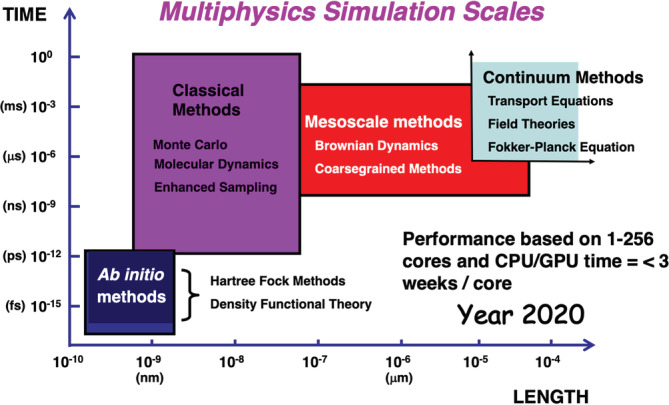
Multiphysics simulations and capabilities of current systems in high‐performance computing platforms available to U.S. researchers such as the extreme science and engineering discovery environment (XSEDE; xsede.org). This figure is inspired and remade from a similar figure in Reference 45 [Color figure can be viewed at wileyonlinelibrary.com]

3.1. Ab initio electronic structure methods

Foundations of electronic structure methods are based on the variational theorem in QM that states that the exact wave function of the ground state of a given Hamiltonian alone is the solution of the variational minimization of the expectation value of the Hamiltonian: minimize 〈Ψ|H|Ψ〉 subject to 〈Ψ|Ψ〉 = 1 yields H|Ψ〉 = E|Ψ〉. In this manner, the variational theorem solves the time‐independent Schrodinger equation, which conforms to the quantum master equation, as noted above. As a practical implementation, one can arrive at very close approximations to the exact ground‐state solution by expanding the wave function in terms of finite basis sets: |Ψ〉 = Σ_i c _i |Φ_i〉. Lynchpin methods that enable the implementation of the variational calculation for many‐electron systems, which are further subject to the constraints of Pauli's exclusion principle, are Hartree–Fock methods,¹⁴ electronic DFT, ⁴⁷ and higher‐order perturbation theory‐based methods. ⁴⁸

Software for quantum chemical calculations are available under open‐source or commercial licenses that make it easy to model molecular systems using electronic structure methods: https://en.wikipedia.org/wiki/List_of_quantum_chemistry_and_solid‐state_physics_software. They have been the driving force to parametrize the force fields of classical simulations such as those in Equation (11) below.

3.2. Molecular dynamics

Molecular dynamics (MD) simulation techniques directly solving Newton's equations of motion are commonly used to model systems of biomolecules and biomaterials because they can track individual atoms and, therefore, answer questions to specific material properties. ⁴⁹ , ⁵⁰ In MD simulations, the starting point is defining the initial coordinates and initial velocities of the atoms characterizing the model system, for example, the desired molecule plus the relevant environment, that is, water molecules or other solvent and/or membranes. The potential of interactions of each of the atoms is calculated using a force field function, which parameterizes the nonbonded and bonded interaction terms of each atom depending on its constituent atom connectivity: bond terms, angle terms, dihedral terms, improper dihedral terms, nonbonded Lennard‐Jones terms, and electrostatic terms. The potential interactions are summed across all the atoms contained in the system to compute an overall potential energy:

$$U\left(\stackrel{\rightharpoonup }{R}\right)=\sum _{\text{bonds}}{K}_{\mathrm{b}}{\left(\mathrm{b}-b_0\right)}^2+\sum _{\text{angles}}{K}_{\theta }{\left(\theta -{\theta }_0\right)}^2+\sum _{\text{dihedrals}}{K}_{\chi }\left(1+\cos \left(\mathit{\eta \chi }-\delta \right)\right)+\sum _{\text{impropers}}{K}_{\varphi }{\left(\varphi -{\varphi }_0\right)}^2+\sum _{\text{nonbonded}}\left({\epsilon }_{\mathit{ij}}\left[{\left(\frac{R_{{\min }_{\mathit{ij}}}}{r_{\mathit{ij}}}\right)}^{12}-{\left(\frac{R_{{\min }_{\mathit{ij}}}}{r_{\mathit{ij}}}\right)}^6\right]\right)+\frac{q_i{q}_j}{{\mathit{\varepsilon r}}_{\mathit{ij}}}.$$ (11)

Constant temperature dynamics are derived by coupling the system to a thermostat using well‐established formulations such as the Langevin dynamics or the Nose–Hoover methodologies. ⁵¹ Application of MD simulations to complex molecules including biomolecules is facilitated by several popular choices of force fields such as CHARMM27 ⁵² (www.charmm.org), AMBER ⁵³ (www.ambermd.org), and GROMOS ⁵⁴ (www.gromacs.org), as well as dynamic simulations packages and visualization/analysis tools such as NAMD ⁵⁵ (www.ks.uiuc.edu/Research/namd/) and VMD ⁵⁶ (www.ks.uiuc.edu/Research/vmd/). MD simulations for commonly modeled molecules such as proteins, nucleic acids, and carbohydrates that have well‐established force fields can be performed directly using a favorite software package such as LAMMPS, GROMACS or HOOMD‐blue (http://glotzerlab.engin.umich.edu/hoomd-blue).

3.3. Monte Carlo methods

In the limit of steady state, the master equation in Equation (1) can be written in matrix form as WP = P or $w_{\mathit{ij}}{P}_j^e=P_i^e$ in the familiar Einstein's convention of, where the summation over the repeated index is implicitly assumed. It is important to recognize is that W is the entire matrix and w _ij is the ijth element of the matrix. Note that w _ij is the transition probability of migrating from microstate j to i, consistent with the definition of w in Equation (1). Similarly, P is the entire vector of probabilities of each microstate, and the ith element of P is P _i, the probability to access microstate i. Note that here, $P_i^e$ is the equilibrium distribution. More generally, if we start with a nonequilibrium state P(1), here (1) is the initial time and the system transitions to later times and is tracked by (2), (3), and so on, then WP(1) = P(2), WP(2) = P(3), WP(3) = P(4), …, WP(n) = P(n + 1), and as n becomes large, P(n) = P(n + 1) = P ^e. In a Monte Carlo (MC) simulation, we simulate the system by sampling accessible microstates according to their equilibrium distribution P ^e, for example, as given by the Boltzmann distribution or the appropriate equivalent distribution in different ensembles (for thermodynamic systems at equilibrium). To achieve this task, we need to choose a W or all w _ij that make up the W, such that $P_i^e$ = exp(−E _i/k _B T)/[Σ_j exp(−E _j/k _B T)] is satisfied. Metropolis et al ⁵⁷ recognized that this could be achieved by choosing w_ij that satisfy equation $w_{\mathit{ij}}{P}_j^e=P_i^e$ by imposing a stronger criterion, namely, $P_m^e{w}_{\mathit{nm}}=P_n^e{w}_{\mathit{mn}}$, which leads to the Metropolis MC method for sampling microstates of a classical system.

Quantum MC techniques provide a direct and potentially efficient means for solving the many‐body Schrödinger equation of QM. ⁵⁸ The simplest quantum MC technique, variational MC, is based on a direct application of MC integration to calculate multidimensional integrals of expectation values such as the total energy. MC methods are statistical, and a key result is that the value of integrals computed using MC converges faster than by using conventional methods of numerical quadrature, once the problem involves more than a few dimensions. Therefore, statistical methods provide a practical means of solving the full many‐body Schrödinger equation by direct integration, making only limited and well‐controlled approximations.

The kinetic Monte Carlo (KMC) method is a MC method computer simulation intended to simulate the time evolution of processes that occur with known transition rates among states (such as chemical reactions or diffusion transport). It is essential to understand that these rates are inputs to the KMC algorithm; the method itself cannot predict them. The KMC method is essentially the same as the dynamic MC method and the Gillespie algorithm. ⁵⁹ From a mathematical standpoint, solving the master equation for such systems is impossible owing to the combinatorially large number of accessible microstates, even considering that the limited number of accessible states renders the transition probability matrix sparse. The Gillespie algorithm provides an ingenious way out of this issue. The practical idea behind KMC is not to attempt to deal with the entire matrix, but instead to generate stochastic trajectories that propagate the system from state to state (i.e., a Markovian sequence of discrete hops to random states happening at random times). From this, the correct time evolution of the probabilities P _i(t) is then obtained by ensemble averaging over these trajectories. The KMC algorithm does so by selecting elementary processes according to their probabilities to fire, followed by an updating of the time.

3.4. Particle‐based mesoscopic models

Earlier, we outlined the connection between the Boltzmann equation (a particular case of the master equation) and the continuum transport equations. However, at the nanoscopic to mesoscopic length scales, neither the molecular description using MD nor a continuum description based on the Navier–Stokes equation are optimal to study nanofluid flows. The number of atoms is too large for MD to be computationally tractable. The microscopic‐level details, including thermal fluctuations, play an essential role in demonstrating the dynamic behavior, an effect which is not readily captured in continuum transport equations. Development of particle‐based mesoscale simulation methods overcomes these difficulties, and the most common coarse‐grained models used to simulate the nanofluid flows are BD, multiparticle collision dynamics, ⁶⁰ and dissipative particle dynamics ⁶¹ , ⁶² , ⁶³ methods. The general approach used in all these methods is to average out relatively insignificant microscopic details in order to obtain reasonable computational efficiency while preserving the essential microscopic‐level details.

In the BD simulation technique, explicit solvent molecules are replaced by a stochastic force, and the hydrodynamic forces mediated by them are accounted for through a hydrodynamic interaction (HI) kernel. The BD equation thus replaces Newton's equations of motion in the absence of inertia:

$$r_i=r_i^0+\sum _j\frac{D_{\mathit{ij}}^{}{F}_j^0}{k_{\mathrm{B}}T}\mathrm{\Delta }t+R_i\left(\mathrm{\Delta }t\right),$$ (12)

where the superscript 0 denotes the value of the variable at the beginning of the time step, r _i is the position of the ith nanoparticle, D _ij is the diffusion tensor, and F _j refers to the force acting on the jth particle. The displacement R _i is the unconstrained Brownian displacement with a white noise having an average value of zero and a covariance of $2D_{\mathit{ij}}^{}\delta \left(t\right)$. The Rotne–Prager–Yamakawa hydrodynamic mobility tensor ⁶⁴ , ⁶⁵ is a commonly employed diffusion tensor to approximate the HIs mediated by the fluid. The trajectories and interactions between the coarse‐grained molecules are calculated using the SDE (Equation (12)), which is integrated forward in time, allowing for the study of the temporal evolution and the dynamics of complex fluids. Stokesian dynamics also represent a class of methods under this paradigm. ⁶⁶

3.5. Continuum models based for fluid flows

We summarize two popular approaches, namely the direct numerical simulations, and lattice Boltzmann methods for solving transport equations.

In direct numerical simulations, a finite element method such as the arbitrary Lagrangian–Eulerian technique can be used to directly solve equations such as Equation (3)) and handle the movement of single‐phase or multiphase domains including particle motions and fluid flow. An adaptive finite element mesh enables a significantly higher number of mesh points in the regions of interest (i.e., close to the particle and wall surfaces compared to the regions farther away). This feature also keeps the overall mesh size computationally reasonable. ⁶⁷

Vast number of flow applications of the lattice Boltzmann method (LBM) have been demonstrated by previous researchers. ⁶⁸ , ⁶⁹ This approach's primary strategy is to incorporate the microscopic physical interactions of the fluid particles in the numerical simulation and reveal the mesoscale mechanism of hydrodynamics. The LBM uses the density distribution functions f(x _i,v _i,t) (similar to the Boltzmann or Liouville equations) to represent a collection of particles with the microscopic velocities v _i and positions x _i at time t, and model the propagation and collision of particle distribution taking the Boltzmann equations for flow and temperature fields into consideration. The LBM solves the discretized Boltzmann equation in velocity space through the propagation of the particle distribution functions f(x,t) along with the discrete lattice velocities e _i and the collision operation of the local distributions to be relaxed to the equilibrium distribution $f_i^0$. The collision term is usually simplified to the single‐relaxation‐time Bhatnagar–Gross–Krook collision operator, while the more generalized multirelaxation‐time collision operator can also be adopted to gain numerical stability. The evolution equation for a set of particle distribution function with a single relaxation time is defined as:

$$f_i\left(x-\mathrm{\Delta }x,t+\mathrm{\Delta }t\right)=f_i\left(x,t\right)-\left(\mathrm{\Delta }t/\tau \right)\left[f_i\left(x,t\right)-{f_i}^0\left(x,t\right)\right]+F_s,$$ (13)

where Δt is the time step, Δx = Δt e _i is the unit lattice distance, and τ is the single‐relaxation time scale associated with the rate of relaxation to the local equilibrium, and F _s is a forcing source term introduced to account for the discrete external force effect. The macroscopic variables such as density and velocity are then obtained by taking moments of the distribution function, that is, $\rho ={\mathrm{\Sigma }}_i{f}_i^{\mathrm{eq}}$ and. As explained earlier, through averaging the mass and momentum variables in the discrete Boltzmann equation, the continuity, and Navier–Stokes equations may be recovered.

Fluctuating hydrodynamics method: As noted in Equation (4), thermal fluctuations are included in the equations of hydrodynamics by adding stochastic components to the stress tensor as white noise in space and time as prescribed by the fluctuating hydrodynamics method. ³⁰ , ⁷⁰ Even though the original equations of fluctuating hydrodynamics are written in terms of stochastic partial differential equations (PDEs), at a very fundamental level, the inclusion of thermal fluctuations always requires the notion of a mesoscopic cell in order to define the fluctuating quantities. The fluctuating hydrodynamic equations discretized in terms of finite element shape functions based on the Delaunay triangulation satisfy the fluctuation–dissipation theorem. The numerical schemes for implementing the thermal fluctuations in the fluctuating hydrodynamics equations are delicate to implement, and obtaining accurate numerical results is a challenging endeavor. ⁷¹

4. PARALLEL AND HIGH‐PERFORMANCE COMPUTING

As noted earlier, a summary of the current capabilities of some of the multiphysics methods on current computing platforms is provided in Figure 1. In order to truly leverage the power of these methods in real‐world applications, one needs to utilize parallel and HPC resources, which we discuss below. In current terms, HPC broadly involves the use of new architectures (such as graphical processing unit [GPU] computing), computing in distributed systems, cloud‐based computing, and computing in parallel to massively parallel platforms or extreme hardware architectures for running computational models (Figure 2). The term applies especially to systems that function with large floating‐point operations per second or systems requiring extensive memory. HPC has remained a sustained and powerful driving force for multiphysics modeling and scientific computing and central to applications in science, engineering, and medicine.

FIGURE 2.

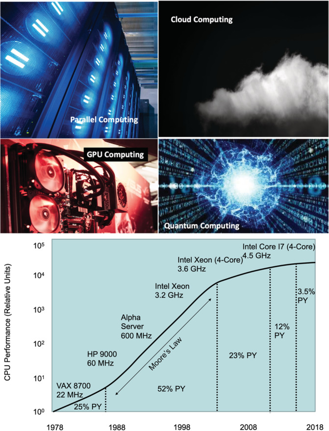
(Top) High‐performance computing (HPC) paradigms—current and future; (bottom) Moore's law and the slow down due to the power wall. This figure is inspired and remade from a similar figure in Reference 72 [Color figure can be viewed at wileyonlinelibrary.com]

A summary of historical developments in parallel and high‐performance computing architectures is sketched in Table 3. The switch to parallel microprocessors is a game‐changer in the history of computing. ⁷⁶ The advances in parallel hardware and software (implementing multiple input multiple date [MIMD] instruction) have torpedoed the advances in multiphysics and multiresolution simulations. This convergence of high‐performance computing and MSM has transformed parallel algorithms (see Table 2), which are the engines of multiphysics modeling.

TABLE 3.

Historical milestones in parallel computing architectures

1842	Parallelism in computing: Menabrea 73
1958–1970	Parallel computers: Burroughs et al 74
1992	Message passing interface as a standard for communication across compute nodes in inherently and massively parallel architectures 75
2005	Establishment of multicore architecture by Intel and others to circumvent the power wall inhibiting Moore's law; standardization of OpenMP (doi: 10.1145/1562764.1562783) (see OpenMP.org)
2007	Release of CUDA: parallel computing platform and application programming interface (API) for graphics processing units (GPUs)

4.1. Multicore architecture and the decline of Moore's law

The linear trends in Figure 2 ceases to hold beyond 2007 prediction due to the power wall in chip architecture. The industry was forced to find a new paradigm to sustain performance enhancement. The viable option was to replace the single power‐inefficient processor with many efficient processors on the same chip, with increasing numbers of processors, or cores, each technology generation every 2 years. This style of the chip was labeled a multicore microprocessor. Hence, the leap to multicore is not based on a breakthrough in programming or architecture and is a retreat from building power‐efficient, high‐clock‐rate, single‐core chips. ⁷⁶ The emergence of the multicore architecture in 2005 prompted shared memory architectures and the establishment of the application programming interface (API), open multiprocessing (OpenMP) standard, which supports multiplatform shared memory multiprocessing programming in C, C++, and Fortran (OpenMP.org).

One of the main drawbacks of MIMD platforms is the high cost of infrastructure. The alternative to MIMD platforms is single‐input multiple data (SIMD) architectures. The use of GPUs in scientific computing has exploded enabled by programing and instructional languages like compute unified device architecture (CUDA), a parallel computing platform and application programming interface or API model created by Nvidia (https://en.wikipedia.org/wiki/CUDA). CUDA allows software developers and software engineers to use a CUDA‐enabled GPU for general‐purpose processing—an approach termed GPGPU (general‐purpose computing on GPUs). The HPC technology is rapidly evolving and is synergistic yet complementary to the development of scientific computing: some useful links on HPC reviews, training, community, and resources are summarized in Table 4.

TABLE 4.

Resources on high‐performance computing (HPC) training, resources, community

Parallel computing: Krste Asanović et al 77

GPU computing: Prandi 78

Cloud computing: Griebel et al 79

HPC virtual workshops and virtual training: https://cvw.cac.cornell.edu/topics

HPC resources: Exascale computing project (https://www.exascaleproject.org/); the extreme science and engineering discovery environment (XSEDE) (https://www.xsede.org); National Science Foundation advanced cyber infrastructure (https://www.nsf.gov/div/index.jsp?div=OAC)

HPC conferences: PEARC (Practice and Experience in Advances in Research and Computing) (https://www.pearc.org/); supercomputing (http://supercomputing.org)

HPC and industry: Intel (https://www.intel.com/content/www/us/en/high‐performance‐computing/overview.html); IBM (https://www.ibm.com/cloud‐computing/xx‐en/solutions/high‐performance‐computing‐cloud/); Google (https://cloud.google.com/solutions/hpc/); Amazon (https://aws.amazon.com/hpc/)

Quantum computing: Steane 80 ; quantum computing emulator on Amazon: (https://aws.amazon.com/braket/)

In Table 2, we mentioned the development of parallel algorithms, which led to a transformation in multiphysics simulations: some examples include parallel matrix operations and linear algebra (https://cvw.cac.cornell.edu/APC/); parallel implementation of the N‐body problem with short‐range interactions (https://cvw.cac.cornell.edu/APC/); long‐range interactions and the parallel particle‐mesh Ewald sum ⁸¹ ; parallel MC ⁸² ; linear‐scaling methods such as multipole expansion ⁸¹ ; linear‐scaling DFT ⁸³ ; parallel graph algorithms (https://cvw.cac.cornell.edu/APC/). As a specific example, we note that the N‐body problem is an essential ingredient in MD. A common goal in MD of large systems is to perform sufficient sampling of the combinatorially large number of conformations available to even the simplest of biomolecules. ⁴² , ⁸⁴ In this respect, a potential disadvantage of MD calculations is that there is an inherent limitation upon the maximum time step used for the simulation (≤2 fs). Solvated systems of biomolecules typically consist of 10⁵–10⁶ atoms. For such system sizes, with current hardware and software, simulation times extending into the tens of microseconds regime is an exceedingly labor‐intensive and challenging endeavor that requires a combination of algorithmic enhancements as well as the utilization of high‐performance computing hardware infrastructure. For example, cutoff distances reduce the number of interactions to be computed without loss of accuracy for short‐range interactions but not for long‐range (electrostatic) interactions; long‐range corrections such as the particle‐mesh Ewald algorithm ⁸⁵ along with periodic boundary conditions are typically implemented for maintaining accuracy. Parallelization techniques enable the execution of the simulations on supercomputing resources such as 4,096 processors of a networked Linux cluster. Although a cluster of this size is a big investment, its accessibility is feasible through the extreme science and engineering discovery environment (XSEDE) for academic researchers. XSEDE resources (www.xsede.org) currently include petaflop of computing capability, and other U.S. national laboratories such as the Oakridge are moving toward exascale computing (https://www.exascaleproject.org). ⁸⁶ Another approach, capitalizing on advances in hardware architecture, is creating custom hardware for MD simulations, and offers one to two orders of magnitude enhancement in performance; examples include MDGRAPE‐3 ⁸⁷ , ⁸⁸ and ANTON. ⁸⁹ , ⁹⁰ GPU‐accelerated computation has recently come into the forefront to enable massive speed enhancements for easily parallelizable tasks with early data indicating that GPU‐accelerated computing may allow for the power of a supercomputing cluster in a desktop, see for example, References 91 and 92.

5. MULTISCALE MODELING 1.0

The acceptance of multiphysics simulation techniques has helped bridge the gap between theory and experiment. ⁹³ Electronic structure (quantum level or ab initio) simulations can reveal how specific molecules assume stable geometrical configurations and charge distributions when subject to a specific chemical environment. By examining the charge distributions and structure, it is possible to quantify and predict structural properties as well as chemical reactivity pertaining to the molecule, which is particularly pertinent when investigating novel materials. Although the quantum simulations provide a wealth of information regarding structure and reactivity, it is currently not possible to model much more than a few hundred atoms at most. MD simulations based on classical (empirical) force fields can model hundreds of thousands of atoms for tens of microseconds in time. Since MD simulations can be set up at atomic resolution, they are uniquely suited to examine thermodynamic and statistical properties of (bio)materials: such properties include (but not limited to) Young's modulus, surface hydration energies, and protein adsorption to different surfaces. ⁹⁴ Coarse‐grained or mesoscale simulations are used to bridge the gap between the atomistic scale of MD simulations and continuum approaches such as elasticity theory or hydrodynamics at the macroscale (i.e., milliseconds, millimeters, and beyond). ⁹³

The ultimate purpose of MSM is to predict the macroscopic behavior from the first principles. Finding appropriate protocols for multiscale simulations is also challenging as either multiphysics simulations need to operate at multiple resolutions, or two or more multiphysics simulations need to be combined. In general, these are achieved via adaptive resolution schemes, coarse‐graining, sequential MSM, concurrent MSM, and enhanced sampling schemes, ⁴⁶ , ⁹⁵ see Table 5.

TABLE 5.

Recipes for multiscale modeling

Enhanced sampling methods 24	Adaptive resolution methods
Umbrella sampling 57	Multiple time step molecular dynamics 96
Parallel tempering 24	Multigrid PDE solvers 71 , 97
Metadynamics 98	Dual resolution 46
Path sampling 99	Equation free methods 100 , 101
Coarse graining methods 102 , 103	Concurrent multiscale methods
Structure matching method 104	QM/MM methods 105
Force matching methods 106	MM/CG methods 107
Energy matching methods 108	CG/CM methods 46
Sequential multiscale methods	Field‐based methods
Parameter passing methods 109	Classical density functional theory 110 , 111
Particle to field passing 112	Polymer field theory 113
Loosely coupled process flow 114 , 115	Memory‐function approach to hydrodynamics 116

The sequential approach links a series of computational schemes in which the operative methods at a larger scale utilize the coarse‐grained (CG) representations based on detailed information attained from smaller‐scale methods. Sequential approaches are also known as implicit or serial methods. The second group of multiscale approaches, the concurrent methods, is designed to bridge multiple individual scales in a combined model. Such a model accounts for the different scales involved in a physical problem concurrently and incorporates some sort of a handshaking procedure to communicate between the scales. Concurrent methods are also called parallel or explicit approaches. Another concept for multiscale simulations is adaptive resolution simulations. Finally, a number of advanced techniques allow for extending the reach of a single‐scale technique such as MD within certain conditions. Such methods offer a route to temporal MSM through enhanced conformational sampling strategies. While these are a lot to review in detail, we summarize these methods into the subclasses followed by references (Table 5) and choose to highlight just some of the more foundational methods below. There is an entire journal dedicated to MSM, Multiscale Modeling and Simulation (https://www.siam.org/journals/mms.php).

5.1. Enhanced sampling methods

The second law of thermodynamics states that natural systems seek a state of minimum free energy at equilibrium. Thus, the computation of a system's free energy is essential in comparing the results of simulation and experiment. Several different methods have been implemented for the calculation of the free energy of various chemical and biomolecular systems, and here we will discuss three of the more commonly employed techniques, namely, the free energy perturbation method ¹¹⁷ and umbrella sampling, ²⁴ and metadynamics.

Free energy perturbation: In molecular systems, the free energy problem is typically presented in terms of computing a free energy difference, ΔF, between two defined thermodynamic states, for example, a ligand‐bound versus unbound molecule. The free energy difference between the two states is expressed as ¹¹⁸ :

$$∆F=-\frac{1}{\beta }\ln {〈\exp \left[-\beta ∆V\left(x\right)\right]〉}_0;\beta =\frac{1}{k_{\mathrm{B}}T},$$ (14)

where the subscript zero indicates configurational averaging over the ensemble of configurations representative of the initial state of the system, k _B is the Boltzmann constant, T is the temperature, and V(x) is the potential energy function that depends on the Cartesian coordinates of the system, (x). ΔF can also be computed by the reverse integration:

$$∆F=-\frac{1}{\beta }\ln {〈\exp \left[-\beta ∆V\left(x\right)\right]〉}_1,$$ (15)

where the subscript one indicates averaging over the ensemble of configurations representative of the final state of the system. However, for systems where the free energy difference is significantly larger, a series of intermediate states must be defined and must differ by no more than 2k _B T. The total ΔF can then be computed by summing the ΔF ^s between the intermediate states:

$$∆F=-\frac{1}{\beta }\sum _{i=1}^{M+1}\ln {〈\exp \left[-\beta \left[V\left(x;{\lambda }_{i+1}\right)-V\left(x;{\lambda }_i\right)\right]\right]〉}_{{\lambda }_i},$$ (16)

where M indicates the number of intermediate states, and λ is the coupling parameter, a continuous parameter that marks the extent of the transition from the initial to the final state. As λ is varied from 0 (initial state) to 1 (final state), the potential energy function V(x; λ) passes from V ₀ to V ₁.

Umbrella sampling: This procedure enables the calculation of the free energy density or potential of mean force (PMF) along an a priori chosen set of reaction coordinates or order parameters, from which free energy changes can be calculated by numerical integration, see, for example, Reference 31. For the free energy calculation, the probability distribution P(S) is calculated by dividing the range of order parameter S into several windows. The histograms for each window are collected by harvesting and binning trajectories in that window, from which the PMF Λ(S) is calculated; the PMF Λ(S) is given by Chandler ¹¹⁹ and Bartels and Karplus, ¹²⁰

$$\mathrm{\Lambda }\left(S\right)=-k_{\mathrm{B}}T\ln \left(P\left(S\right)\right)+\text{Constant};\text{then},\exp \left(-\beta \mathrm{\Delta }F\right)=\int \exp \left(-\beta {\mathrm{\Lambda }}_i\left(S\right)\right)\mathit{dS}.$$ (17)

The functions Λ(S) in different windows are pieced together by matching the constants such that the Λ function is continuous at the boundaries of the windows. Thus, the arbitrary constant associated with each window is adjusted to make the Λ function continuous. Note that Λ(S) here is the same function as F(S) in Equation (6). The error in each window of the PMF calculations is estimated by dividing the set of trajectories into two blocks and collecting separate histograms. The calculation of the multidimensional PMF (multiple reaction coordinates) using the weighted histogram analysis method reviewed by Roux, ¹²¹ which enables an easy and accurate recipe for unbiasing and combining the results of umbrella sampling calculations, which simplifies considerably, the task of recombining the various windows of sampling in complex systems and computing ΔF.

Metadynamics: In metadynamics, the equations of motion are augmented by a history‐dependent potential V(S,t) = k _BΔT[1 + N(S,t)/τ], where N(S,t) represents the histograms of previously visited configurations up to time t. With this choice of the biasing potential, the evolution equation of V is derived and is solved together with the equation of motion. One can show that the unbiased free energy can be constructed from the biased dynamics using the equation F(S) = [(T + ΔT)/ΔT]V(S). Metadynamics accelerates rare events along chosen CVs S. Well‐tempered metadynamics ⁹⁸ , ¹²² is widely used to sample the large‐scale configurational space between the configurations in large biomolecular systems.

Methods for determining reaction paths: Path‐based methodologies seek to describe transition pathways connecting two well‐defined states ¹²³ , ¹²⁴ , ¹²⁵ ; practical applications of this ideology are available through methods such as stochastic path approach, ¹²⁶ nudged elastic band, ¹²⁷ , ¹²⁸ , ¹²⁹ finite temperature string, ¹³⁰ and transition path sampling, ⁹⁹ , ¹³¹ , ¹³² which each exploit the separation in timescales in activated processes, namely, the existence of a shorter time scale of relaxation at the kinetic bottle neck or the transition state (τ _relax), in comparison with a much longer timescale of activation at the transition state itself (τ _TS). Below, we review the path‐based method of transition path sampling.

Transition path sampling ⁹⁹ , ¹³¹ aims to capture rare events (excursions or jumps between metastable basins in the free energy landscape) in molecular processes by essentially performing MC sampling of dynamics trajectories; the acceptance or rejection criteria are determined by selected statistical objectives that characterize the ensemble of trajectories. In transition path sampling, time‐reversible MD trajectories in each transition state region are harvested using the shooting algorithm ¹³² to connect two metastable states via a MC protocol in trajectory space. Essentially, for a given dynamics trajectory, the state of the system (i.e., Basin A or B) is characterized by defining a set of order parameters χ = [χ ₁, χ ₂, …]. Each trajectory is expressed as a time series of length τ. To formally identify a basin, the population operator h _A = 1 if and only if a particular molecular configuration associated with a time t of a trajectory belongs to Basin A; otherwise h _A = 0. The trajectory operator H _B = 1 if and only if the trajectory visits Basin B in duration τ, that is, there is at least one time slice for which h _B = 1; otherwise H _B = 0. The idea in transition path sampling is to generate many trajectories that connect A to B from one such existing pathway. This is accomplished by a Metropolis algorithm that generates an ensemble of trajectories [χ ^τ] according to a path action S[χ ^τ] given by S[χ ^τ] = ρ(0)h _A(χ ₀)H _B[χ ^τ], where ρ(0) is the probability of observing the configuration at t = 0 (ρ(0)∝exp(−E(0)/k _B T), in the canonical ensemble). Trajectories are harvested using the shooting algorithm ¹³² : a new trajectory χ*^τ is generated from an existing one χ ^τ by perturbing the momenta of atoms at a randomly chosen time t in a symmetric manner, ¹³² that is, by conserving detailed balance. The perturbation scheme is symmetric, that is, the probability of generating a new set of momenta from the old set is the same as the reverse probability. Moreover, the scheme conserves the equilibrium distribution of momenta and the total linear momentum (and, if desired, the total angular momentum). The acceptance probability implied by the above procedure is given by P _acc = min(1, S[χ*^τ]/S[χ ^τ]). With sufficient sampling in trajectory space, the protocol converges to yield physically meaningful trajectories passing through the true transition‐state (saddle) region.

5.2. Coarse graining

Coarse‐grained molecular dynamics (CGMD) simulations employ intermediate resolution in order to balance chemical detail with system size. They offer sufficient size to study membrane‐remodeling events while retaining the ability to self‐assemble. Because they are capable of simulating mesoscopic length scales, they make contact with a wider variety of experiments. A complete coarse‐grained model must include two components: a mapping from atomistic structures to coarse‐grained beads and a set of potentials that describe the interactions between beads. The former defines the geometry or length scale of the resulting model, while the latter defines the potential energy function or the force field. The parameterization of the force field is essential to the performance of the model, which is only relevant insofar as it can reproduce experimental observables. Here we will describe the characteristic methods for developing CGMD models, namely, the bottom‐up structure‐ and force‐matching and top‐down free energy‐based approaches. We note that excellent reviews have been written on coarse‐grained methods with applications in other fields such as polymer physics, see, for example, Reference 102.

Structure and energy matching: Klein and coworkers developed a coarse‐grained model for phospholipid bilayers by matching the structural and thermodynamic properties of water, hydrocarbons, and lipid amphiphile to experimental measurements and all‐atom simulations. ¹³³ The resulting force field, titled CMM‐CG, has been used to investigate a range of polymer systems as well as those containing nonionic liquids and lipids. Classic coarse‐grained methods propose pair potentials between CG beads according to the Boltzmann inversion method. In this method, a pair correlation function, or radial distribution function g(r) defines the probability of finding a particle at distance r from a reference particle such that the conditional probability of finding the particle is ρ(r) = ρg(r), where ρ is the average number density of the fluid. The PMF between CG beads is then estimated by Equation (18) where g _aa(r) is measured from atomistic simulation, and α _n is a scaling factor (corresponding to the nth iteration of the estimate) designed to include the effect of interactions with the (necessarily) heterogeneous environment.

$$V_n\left(r\right)={\alpha }_n\left\{-k_{\mathrm{B}}T\ln \left(g_{\mathrm{aa}}\left(r\right)\right)\right\}.$$ (18)

The Boltzmann inversion method is iteratively corrected according to Equation (19) to correct the tabulated potentials until the pair‐correlation functions for the atomistic and coarse‐grained systems agree.

$$V_{n+1}\left(r\right)=V_n\left(r\right)+k_{\mathrm{B}}T\ln \frac{g_n\left(r\right)}{g_{\mathrm{aa}\left(r\right)}}.$$ (19)

Force matching: The method of force matching provides a rigorous route to developing a coarse‐grained force field directly from forces measured in all‐atom simulations. In so far as the multibody coarse‐grained PMF is derived from structure factors that depend on temperature, pressure, and composition, they cannot be transferred to new systems. To avoid this problem, the force‐matching approach proposes a variational method in which a coarse‐grained force field is systematically developed from all‐atom simulations under the correct thermodynamic ensemble. ¹³⁴ In the statistical framework developed by Izvekov and Voth, ¹³⁴ , ¹³⁵ , ¹³⁶ it is possible to develop the exact many‐body coarse‐grained PMF from a trajectory of atomistic forces with a sufficiently detailed set of basis functions.

The method starts with a collection of sampled configurations from an atomistic simulation of the target system and calculates the reference forces between atoms of a particular type. After decomposing their target force into a short‐ranged part approximated by a cubic spline and a long‐ranged Coulomb part one solves the overdetermined set of linear equations given by Equation (20):

$$\sum _{\beta =1}^K\sum _{j=1}^{N_{\beta }}\left(-f\left(r_{\mathit{\alpha il},\mathit{\beta jl},}\left\{r_{\mathit{\alpha \beta },\kappa }\right\},\left\{f_{\mathit{\alpha \beta },\kappa }\right\},\left\{f_{\mathit{\alpha \beta },\kappa }^{″}\right\}\right)-\frac{q_{\mathit{\alpha \beta }}}{r_{\mathit{\alpha il},\mathit{\beta jl}}^2}\right)n_{\mathit{\alpha il},\mathit{\beta jl}}=F_{\mathit{\alpha il}}^{\mathrm{ref}}.$$ (20)

In Equation (20), the r _αβ,κ correspond to the spline mesh at points κ for pairs of atoms of types α and β, while f and f″ are spline parameters that ensure continuous derivatives f′(r) at the mesh points and define the short‐ranged part of the force. The subscript α _il labels the ith atom of type α in the lth sampled atomic configuration. Solving these equations minimizes the Euclidean norm of vectors of residuals and can be solved on a minimal set of atomistic snapshots using a singular value decomposition algorithm. By adding the Coulomb term to the short‐ranged potential above, this technique allows for the inclusion of explicit electrostatics. The method reproduces site‐to‐site radial distribution functions from atomistic MD simulations in the as well as the density profiles in inhomogeneous systems such as lipid bilayers.

The energy‐based approach of the Martini force field: The Martini force field developed by Marrink and coworkers eschews systematic structure‐matching in pursuit of a maximally transferable force field which is parameterized in a “top‐down” manner, designed to encode information about the free energy of the chemical components, thereby increasing the range of thermodynamic ensembles over which the model is valid. ¹⁰⁸

The Martini model employs a four‐to‐one mapping of water and non‐hydrogen atoms onto a single a bead, except in ring‐like structures, which preserve geometry with a finer‐scale mapping. Molecules are built from relatively few bead types, which are categorized by polarity (polar, nonpolar, apolar, and charged). Each type is further distinguished by hydrogen bonding capabilities (donor, acceptor, both, or none) as well as a score describing the level of polarity. Like the methods described above, Lennard‐Jones parameters for nonbonded interactions are tuned for each pair of particles. These potentials are shifted to mimic a distance‐dependent screening effect and increase computational efficiency. Charged groups interact via a Coulomb potential with a low relative dielectric for explicit screening. This choice allows the use of full charges while reproducing salt structure factors seen in previous atomistic as well as the hydration shell identified by neutron diffraction studies. Nonbonded interactions for all bead types are tuned to semi‐quantitatively match measurements of density and compressibility. Bonded interactions are specified by potential energy functions that model bonds, angles, dihedrals with harmonic functions, with relatively weak force constants to match the flexibility of target molecules at the fine‐grained resolutions. The Martini force field's defining feature is the selection of nonbonded parameters that are optimized to reproduce thermodynamic measurements in the condensed phase. Specifically, the Martini model semi‐quantitatively reproduces the free energy of hydration, the free energy of vaporization, and the partitioning free energies between water and a collection of organic phases, obtained from the equilibrium densities in both phases. ¹⁰⁸

5.3. Minimal coupling methods

Minimal coupling methods minimize explicit and concurrent communication across scales via a variety of clever algorithmic or software architecture tricks and represent a power repertoire of multiscale methods. There are numerous techniques in this popular category, and we chose not to delve into any of them in detail. A few of the methods in these categories are listed along with their references in Table 5 under sequential multiscale methods and adaptive resolution methods. Sequential methods involve computing a property or a constitutive relationship at one (typically the molecular) scale and employing (either pre‐ or on‐the‐fly‐) computed values in the other (typically the continuum scale). ¹²¹ , ¹²⁵ , ¹²⁶

5.4. Concurrent multiscale methods

The concurrent approaches couple two or more methods and execute them simultaneously with continuous information transfer across scales in contrast to the minimal coupling methods that attempt to do the opposite. In this class of methods, the behavior at each scale depends strongly on the phenomena at other scales. A successful algorithm in the concurrent method implements a smooth coupling between the scales. In concurrent simulations, often, two distinct domains with different scales are linked together through a buffer or overlap region called the handshake region. ⁴⁶

Quantum mechanics/molecular mechanics (QM/MM) simulations: An example of concurrent include mixed QM/MM methods combining MD using the empirical force field approach with electronic structure methods ⁴⁷ , ⁴⁸ , ¹³⁷ to produce a concurrent multiscale method. ¹⁰⁵ , ¹³⁸ , ¹³⁹ , ¹⁴⁰ , ¹⁴¹ , ¹⁴² , ¹⁴³ , ¹⁴⁴ , ¹⁴⁵ , ¹⁴⁶ , ¹⁴⁷ , ¹⁴⁸ , ¹⁴⁹ In the QM/MM simulations, the system is subdivided into two subregions, the QM subregion (QM region) where the reactive events take place, and the MM subregion (which provides the complete environment around the reactive chemistry). ¹³⁹ , ¹⁴¹ Since electronic structure methods are limited by the number of atoms they can handle (typically 50–500), the QM subregion is restricted to a small number of atoms of the total system. For example, in an enzymatic system, the quantum region can consist of Mg²⁺ ions, water molecules within 3 Å of the Mg²⁺ ions, parts of the substrate molecules, and the catalytic amino acid residues (such as aspartic acids). The remaining protein and solvent molecules are treated classically using the regular classical force field.

In QM/MM simulations, wave function optimizations are typically performed in the quantum (or QM) subregion of the system using an electronic structure method such as DFT. ⁴⁷ In this step, the electrostatic coupling between the QM and the MM subregions is accounted for, that is, the charges in the MM subregion are allowed to polarize the electronic wave functions in the QM subregion. The forces in the quantum subregion are calculated using DFT on‐the‐fly, assuming that the system moves on the Born–Oppenheimer surface. ¹⁴¹ , ¹⁵⁰ That is, we assume a clear timescale of separation between the electronic and nuclear degrees of freedom and the electronic degrees of freedom are in their ground state around the instantaneous configurations of the nuclei. The forces on the classical region are calculated using a classical force field. Besides, a mixed Hamiltonian (energy function) accounts for the interaction of the classical and the quantum subregions. For example, since the QM/MM boundary often cuts across covalent bonds, one can use a link atom procedure ¹⁴⁴ to satisfy the valences of broken bonds in the QM subregion. Also, bonded terms and electrostatic terms between the atoms of the QM region and those of the classical region are typically included. ¹⁴²

From a practitioner's standpoint, QM/MM methods are implemented based on existing interfaces between the electronic structure and the MD programs; one example implementation is between GAMESS‐UK ¹⁵¹ (an ab initio electronic structure prediction package) and CHARMM. ⁵² The model system can then be subjected to the usual energy minimization and constant temperature equilibration runs at the desired temperature using the regular integration procedures in operation for pure MM systems; it is customary to carry out QM/MM dynamics runs (typically limited to 10–100 × 10⁻¹² s because of the computationally intensive electronic structure calculations) using a standard 1‐fs time step of integration. The main advantage of the QM/MM simulations is that one can follow reactive events and dissect reaction mechanisms in the active site while considering the explicit coupling to the extended region. In practice, sufficient experience and care are needed in the choices of the QM subregion, and the many alternative choices of system sizes, as well as the link‐atom schemes, need to be compared to ensure convergence and accuracy of results. ¹⁴² The shorter length of the dynamics runs in the QM/MM simulations (10⁻¹² s) relative to the MD simulations (10⁻⁹ s) implies that sufficiently high‐resolution structures are usually necessary for setting up such runs as the simulations only explore a limited conformational space available to the system. Another challenge is an accurate and reliable representation of the mixed QM/MM interaction terms. ¹⁴⁵ These challenges are currently being overcome by the suitable design of next‐generation methods for electronic structure and MM simulations. ⁸³ , ¹⁵² Other examples of concurrent methods linking electronic structure and or MM scales include Car–Parrinello MD ¹⁵³ , ¹⁵⁴ and mixed molecular mechanics/coarse‐grained (MM/CG). ¹⁰⁷ , ¹⁵⁵

Linking atomistic and continuum models: In several applications involving solving continuum equations in fluid and solid mechanics, there is a need to treat a small domain at finer (often molecular or particle‐based resolution) to avoid sharp fronts or even singularities. In such cases linking atomistic and continuum domains using bridging algorithms are necessary. A class of algorithms that realize this challenging integration have been reviewed in Reference 46: examples include the quasicontinuum approach, finite‐element/atomistic method, bridging scale method, and the Schwartz inequality method, ¹⁵⁶ , ¹⁵⁷ which all employ domain decomposition bridging by performing molecular scale modeling in one (typically a small domain) and integrating it with continuum modeling in an adjoining (larger) domain, such that certain constraints (boundary conditions) are satisfied self‐consistently at the boundary separating the two domains. Such approaches are useful for treating various problems involving contact lines.

5.5. Field‐based coarse‐graining

For specific systems such as nanoparticle and nanofluid transport, both molecular interactions (due to biomolecular recognition) and HIs (due to fluid flow and boundary effects) are significant. The integration of disparate length and time scales does not fit traditional multiscale methods. The complexity lies in integrating fluid flow and memory for multiphase flow in complex and arbitrary geometries, while simultaneously including thermal and stochastic effects to simulate quasi‐equilibrium distributions correctly to enable receptor–ligand binding at the physiological temperature. This issue is ubiquitous in multivalent binding or adhesive interactions between nanoparticles and cells or between two cells. Bridging the multiple length scales (from meso to molecular) and the associated time scales relevant to the problem is essential to success herein. Multiple macroscopic and mesoscopic time scales governing the problem include (a) hydrodynamic time scale, (b) viscous/Brownian relaxation time scale, and (c) Brownian diffusion time scale.

Memory function approach to coarse‐graining with HIs: In the description of the dynamics of nanosized Brownian particles in an bounded and unbounded fluid domains the memory functions decay with algebraic correlations as enumerated by theoretical and computational studies. ⁷¹ , ¹¹⁶ , ¹⁵⁸ The equation of stochastic motion for each component of the velocity of a nanoparticle immersed in a fluid in bounded and unbounded domains takes the form of a GLE of the form of Equation (9); to account for HI, a composite GLE was introduced. ¹⁵⁹ , ¹⁶⁰

$$\begin{array}{l}M\frac{\mathit{dU}\left(x,t\right)}{\mathit{dt}}=-6\mathit{\text{πηβU}}\left(x,t\right)-A_1\left(t\right){\int }_{-\infty }^t\left({\left|t-t^{\prime }\right|}^{-3/2}U\left(x,t^{\prime }\right)d{t}^{\prime }\right)\\ -A_2\left(t\right){\int }_{-\infty }^t\left({\left|t-t^{\prime }\right|}^{-5/2}U\left(x,t^{\prime }\right)d{t}^{\prime }\right)-\frac{\mathit{dF}}{\mathit{dx}}+R\left(t\right).\end{array}$$ (21)

Here M is the added mass, and β is the geometric factor with wall effect corrections, the integrands include the memory functions associated with the velocity autocorrelation functions in different domains (lubrication, bulk, and near‐wall regimes in order of the first three terms on the right‐hand side). The fourth term on the right‐hand side is the force from other thermodynamic potentials, same as F(S) in Equation (7), and the fifth term is the random force term with colored noise to be consistent with the fluctuation–dissipation theorem for composite GLE. ¹⁵⁹ , ¹⁶⁰

Effect of molecular forces is introduced as forcing functions in the GLE ¹⁵⁹ and the effect of multiple particles including multiparticle HI can be introduced via DFT‐based treatments ¹¹⁰ , ¹¹¹ to define F(S) from hydrodynamic and colloidal effects in addition to the specific contributions from molecular forces. If the memory functions are unknown, they can be obtained via deterministic approaches by solving the continuum hydrodynamic equations numerically. ⁷¹ , ¹⁵⁸ These disparate hydrodynamic fields and molecular forces can be integrated into a single GLE to realize a unified description of particle dynamics under the influence of molecular and hydrodynamic forces. ¹¹⁶ Another approach to integrating these forces is via the Fokker Planck approach using the sequential multiscale method paradigm. ¹⁶¹

6. MULTISCALE MODELING 2.0

6.1. Integrating MSM and ML to elucidate the emergence of function in complex systems

We are riding the wave of a paradigm shift in the development of MSM methods due to rapid development and changes in HPC infrastructure (see Figure 2) and advances in ML methods. Thus, MSM and HPC have emerged as essential tools for modeling complex problems at the microscopic scales with a focus on leveraging the structured and embedded physical laws to gain a mechanism‐based understanding. This success notwithstanding, the design of new MSM algorithms in coupling different scales, data utilization, and their implementation on HPC is becoming increasingly cumbersome in the face of heterogeneous data availability and rapidly evolving HPC architectures and platforms. On the other hand, while purely data‐driven models of molecular and cellular systems spawned by the techniques of data science, ¹⁶² , ¹⁶³ , ¹⁶⁴ and in particular, ML methods including deep learning methods, ¹⁶⁵ , ¹⁶⁶ , ¹⁶⁷ are easy to train and implement, the underlying model manifests as a black box. This general approach taken by the ML community is well suited for classification, learning, and regression problems, but suffers from limitations in interpretability and explainability, especially when mechanism‐based understanding is a primary goal. There lies a vast potential in combining MSM, HPC, and ML methods with their complementary strengths. ⁴ MSM models are routinely coupled together by appropriately propagating information across scales (see Section 5), while the ever‐increasing advances in hardware capabilities and high‐performance software implementations allows us to study increasingly more complex phenomena at a higher fidelity and higher resolution. While much of the discussion thus far has been focused on MSM and HPC methods, the progress and potential in integrating MSM and ML are discussed below and represent the forefront of emerging MSM research, in which we discuss a few emerging integrative approaches to combine ML and MSM.

6.2. Integrators and autotuning

Over the past two decades, MSM has emerged into a promising tool to build in silico predictive models by systematically integrating knowledge from the tissue, cellular, and molecular level. Depending on the scale of interest, governing equations in each scale of the MSM approaches may fall into two categories, ordinary differential equation‐based and PDE‐based approaches. Examples include MD, ⁴⁹ coarse‐grained mesoscale models, ¹⁰³ lattice Boltzmann methods, ⁶⁸ immersed boundary methods, ¹⁶⁸ as well as classical finite element approaches. ¹⁶⁹ ML‐based methods can speed up, optimize, and autotune several of the existing solvers for multiphysics simulations. ¹⁷⁰ , ¹⁷¹

6.3. ML‐enabled MSM

As noted earlier, one of the main objectives of MSM is to couple the physics at different scales using bridging algorithms that pass information between two scales, such as in QM/MM, MM/CG, coarse‐grained continuum (CG/CM), and field‐based methods discussed in Section 5. However, the implementation of this methodology on parallel supercomputing HPC architectures is complicated and cumbersome. To address this significant limitation in implementation, we advocate for an ML‐enabled integration or bridging of scales as a viable approach to develop the next‐generation of MSM methods to achieve maximal efficiency and flexibility in integrating scales.

Here one can leverage ongoing developments in ML to accelerate the prediction of large‐scale computational models. As a viable path forward, ML workflow can be implemented in three steps (see Figure 3) ⁴ : (1) train deep neural network (NN) encoders that connect properties of the MSM model at Scale 1 (e.g., MD or MC) to those at Scale 2 (e.g., continuum model), using explicit MSM computations overextended parameter sets to cover all possible conditions; (2) implement the encoders in place of the coupling algorithms to bridge Scales 1 and 2; (3) ensure that the properties profiles obtained from the two scales match by defining a cost‐function that constrains the training of NNs in (1). The NN‐based coupling of scales is expected to be robust, computationally efficient for MSM algorithms.

FIGURE 3.

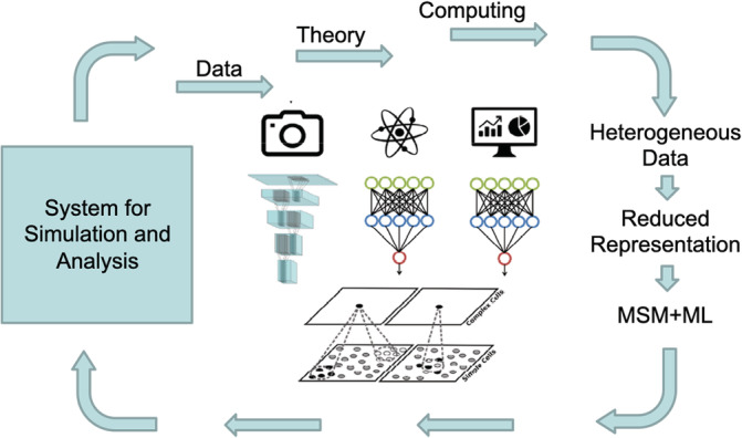
The proposed synergy of multiscale and machine learning aspires to (a) accelerate the prediction of large‐scale computational models, (b) discover interpretable models from irregular and heterogeneous data of variable fidelity, and (b) guide the judicious acquisition of new information towards elucidating the emergence of function in biological systems. This figure is inspired and remade from a similar figure in Reference 4 [Color figure can be viewed at wileyonlinelibrary.com]

One challenge is to discover interpretable models from heterogeneous data of variable fidelity and guide the judicious acquisition of new information toward elucidating the emergence of function in biological systems. This challenge can be addressed by subjecting the entire MSM model to contemporary data science and statistical methodologies, that is, ¹⁷² sensitivity, ¹ evolvability, ² robustness ¹⁷³ analyses, uncertainty quantification, ¹⁷⁴ multifidelity modeling, ⁴ and pattern discovery and model reduction. ¹⁷⁵

6.4. Physics‐informed NN (PINN)

Can we use prior physics‐based knowledge to avoid overfitting or nonphysical predictions? From a conceptual point of view, can we supplement ML with a set of known physics‐based equations, an approach that drives MSM models in engineering disciplines? While data‐driven methods can provide solutions that are not constrained by preconceived notions or models, their predictions should not violate the fundamental laws of physics. There are well‐known examples of deep learning NNs that appear to be highly accurate but make highly inaccurate predictions when faced with data outside their training regime, and others that make highly inaccurate predictions based on seemingly minor changes to the target data. ¹⁷⁶ To address this ubiquitous issue of purely ML‐based approaches, numerous opportunities to combine ML and MSM toward a priori satisfying the fundamental laws of physics, and, at the same time, preventing overfitting of the data.

A potential solution is to combine deterministic and stochastic models. Coupling the deterministic governing equations MSM models—the balance of mass, momentum, and energy—with the stochastic equations of systems biology and biophysical systems—cell‐signaling networks or reaction–diffusion equations—could help guide the design of computational models for otherwise ill‐posed problems. Physics‐informed NNs ¹⁷⁷ is a promising approach that employs deep NNs and leverages their well‐known capability as universal function approximators. ¹⁷⁸ In this setting, we can directly tackle nonlinear problems without the need for committing to any prior assumptions, linearization, or local time stepping. PINNs exploit recent developments in automatic differentiation ¹⁷⁹ to differentiate NNs concerning their input coordinates and model parameters to obtain physics informed NNs. Such NNs are constrained to respect any symmetry, invariance, or conservation principles originating from the physical laws that govern the observed data, as modeled by general time‐dependent and nonlinear PDEs. This construction allows us to tackle a wide range of problems in computational science and introduces a potentially disruptive technology leading to the development of new data‐efficient and physics‐informed learning machines, new classes of numerical solvers for PDEs, as well as new data‐driven approaches for model inversion and systems identification.

6.5. Deep NN algorithms inspired by statistical physics and information theory

Large amounts of data, cheap computation, and efficient algorithms are driving the impressive performance and adoption of robust deep learning architectures. However, building, maintaining, and expanding these systems is still decidedly an art and requires a lot of trial and error. Learning and inference methods have a history of being inspired by and derived from the principles of statistical physics and information theory. ¹⁸⁰ , ¹⁸¹ We summarize examples to advance this theme to derive NN algorithms based on a confluence of ideas in statistical physics and information theory ¹⁸² and to feed them back into core MSM methods by prescribing new computational techniques for deep NNs. (A) Generalization in deep NN: the approach utilizes algebraic topology ¹⁸³ , ¹⁸⁴ to characterize the space of reachable functions using stochastic dynamics on data in order to build computationally efficient architectures and algorithms to train them. ¹⁸⁵ , ¹⁸⁶ , ¹⁸⁷ (B) Characterizing the quality of representations and the performance of encoders, decoders: Recent works have proposed to exploit principles of representation learning to formulate variational approaches for the assessment of performance in deep learning algorithms ³⁴ that provide guarantees on the performance of the final model.

6.6. ML‐enhanced conformational sampling

Advances in ML‐derived force fields are promising to revolutionize classical simulations by directly defining energy landscapes from more accurate QM simulations. ¹⁸⁸ , ¹⁸⁹ Besides, in particle‐based simulations of MSM, the efficient sampling of high‐dimensional conformational spaces constitutes a significant challenge in the computational molecular sciences limiting the longtime MD simulations of molecular systems in biophysical chemistry and materials science. Combining MD simulations with ML can provide a powerful approach to address the challenges mentioned above. ¹⁹⁰ The last decade has seen significant advances in the use of electronic structure calculations to train ML potentials for atomistic simulations capable of reaching large systems sizes and longtime scales with accurate and reliable energies and forces. More recently, ML approaches have proved useful in learning high‐dimensional free energy surfaces, ¹⁹¹ , ¹⁹² and in providing a low dimensional set of CVs. ¹⁹³ Some examples are discussed below.

Boltzmann generators: The primary difficulty in sampling physical realizations or microstates of the system from the Boltzmann distribution lies in the nature of the potential energy. In large, complex systems, the conformational space holds the positions of hundreds of thousands to millions of atoms. The potential energy should be viewed as a vast, rugged landscape in this high‐dimensional space characterized by an exponentially large number of low‐energy regions or minima, all separated by ridges. It is now possible to train a deep NN to learn a transformation from the conformational space to another variable space such that in this new space, the variables are distributed according to simple distributions such as the Gaussian distribution. One can backmap to the original space through inverse transformation onto a high‐probability region of the original conformational space. ¹⁹⁰

ML‐enabled conformational enhanced sampling: The choice of appropriate CVs (aka order parameters in the earlier section) for enhanced sampling methods such as meta‐dynamics is still a challenge. Recent advances have enabled ML tools of supervised learning to define appropriate CVs. The pipeline flow for such supervised ML methods utilizes ML‐identified features from (A) as CVs for enhanced sampling simulations. ¹⁹⁴ Another choice for ML‐identified CV is through the use of variational autoencoders, ¹⁹⁵ which are deep NNs that perform dimensionality reduction similar to principal component analysis. The neural encoder takes a high dimensional input vector and outputs a lower‐dimensional output vector. The neural decoder then takes the latent variable as input and attempts to reconstruct the original high dimensional input using standard optimization techniques of a loss function. ¹⁹⁶

ML‐enhanced adaptive path sampling: While enhanced sampling methods are efficient in exploring the landscape based on predefined CVs, one often discovers new variables during sampling. In such scenarios, new variables that become relevant are often orthogonal to the original CVs, and it is impossible to incorporate such variables adaptively into the free energy landscape. One approach is to combine enhanced sampling such as metadynamics with path sampling and utilize the newly identified CVs in the path sampling through a path action. ¹⁹⁷ In this approach, path sampling is pursued by adaptively modifying the path action, and the free energy landscape based on the original CVs can be refined iteratively. The path action approach is also easily customized to include other ML strategies such as reinforcement learning to guide the system through non‐Boltzmann paths.

6.7. Ab initio methods using quantum computing

Quantum computers hold promise to enable efficient simulations of the properties of molecules and materials; however, at present, their abilities are limited due to a limited number of qubits that can be realized. In the near‐term, the throughput of quantum computers is limited by the small number of qubits available, which prohibits large systems. It is more practical to develop hybrid quantum‐classical methods where the quantum computation is restricted to a small portion of the system; for example, molecules where an active region requires a higher level of theoretical accuracy than its environment. Galli et al outline a quantum embedding theory for the calculation of strongly correlated electronic states of active regions, with the rest of the system described within DFT. ¹⁹⁸ The authors demonstrate the efficacy of the method by investigating defect quantum bits in semiconductors that are of great interest for quantum information technologies. The calculations are performed on quantum computers and show that they yield results in agreement with those obtained with exact diagonalization on classical architectures, paving the way to simulations of realistic materials on near‐term quantum computers.

7. CONCLUSIONS

Amidst the explosion of data in all walks of science, engineering, biology, and biomedical science, it is useful to seek an interpretable basis for the emergence of function. How can geometry, physics, and engineering best inform biology or lead to the discoveries of new functional advanced materials? The complex multiscale interactions that characterize the dynamic behavior of biological systems ¹⁹⁹ and advanced materials have limited our ability to understand the fundamental mechanisms behind the emergence of function to relatively idealized systems. ²⁰⁰

ML integrated with MSM is poised to enhance the capabilities of standard MSM approaches profoundly, particularly in the face of increasing problem complexity and data intensiveness. The contemporary research problems warrant an interdisciplinary environment to tackle emerging scientific and technological grand‐challenge problems that carry substantial societal impact. Research projects, while posed across varied application domains in science and engineering, often have common features: (a) the problem/solution spans diverse length and timescales and benefits from MSM, (b) ML methods integrate into the MSM methods to define the new approaches at the frontiers of MSM development, (c) tools of data science are effectively leveraged to integrate experimental data with the proposed model, and (d) the implementation of the model will utilize HPC methods and/ or platforms. Foundational training for future scholars should ideally provide: (a) working knowledge in fundamental science and modeling methodologies at multiple lengths and timescales spanning the molecular to process scales; (b) the requisite skills to integrate, and couple multiple scales into a multiscale paradigm; (c) learnings to exploit elements of data science, including ML methods and tools of data integration from cloud‐based, data‐rich repositories in order to validate and test computational models and software; (d) learnings to combine the rich tools of ML with MSM methods to define the next‐generation of MSM methods; (e) experience to adopt, and implement best practices in software architecture to leverage modern computational infrastructure and develop efficient sustainable codes. With these foundations and skill sets in the arsenal of the emerging researcher, the potential to blend MSM, HPC, and ML presents opportunities for unbound innovation and represents the future of MSM and explainable ML that will likely define the fields in the 21st century.

Radhakrishnan R. A survey of multiscale modeling: Foundations, historical milestones, current status, and future prospects. AIChE J. 2021;67:e17026. 10.1002/aic.17026

REFERENCES

- 1. Sobol IM. Sensitivity estimates for nonlinear mathematical models. Math Model Comput Exp. 1993;1(4):407‐414. [Google Scholar]
- 2. Brown KS, Sethna JP. Statistical mechaniccl approaches to models with too many unknown parameters. Phys Rev E. 2003;68:021904. [DOI] [PubMed] [Google Scholar]
- 3. Ghosh A. A Heterogeneous and Multiscale Modeling Framework to Develop Patient‐Specific Pharmacodynamic Systems Models in Cancer. [PhD Thesis]. Philadelphia, PA: University of Pennsylvania; 2019.
- 4. Alber M, Buganza Tepole A, Cannon WR, et al. Integrating machine learning and multiscale modeling—perspectives, challenges, and opportunities in the biological, biomedical, and behavioral sciences. npj Digital Med. 2019;2(1):115. [DOI] [PMC free article] [PubMed] [Google Scholar]
- 5. Newton I. Laws of motion in classical mechanics. Principia Math. 1687. [Google Scholar]
- 6. Liouville J. Liouville theorem. J Math. 1838;3:342. [Google Scholar]
- 7. Navier CL. Navier Stokes Equation. Paris: Chez Carilian‐Goeury; 1838. [Google Scholar]
- 8. Maxwell JC. Maxwell's equations of electrodynamics. Philos Trans Roy Soc Lond. 1865;155:459‐512. [Google Scholar]
- 9. Boltzmann L. Boltzmann equation. Sitzungsber Akade Wissen. 1872;66:275‐370. [Google Scholar]
- 10. Stokes GG. Navier Stokes Equation. Cambridge: Cambridge University Press; 1880:75‐129. [Google Scholar]
- 11. Langevin P. Langevin equation. C R Acad Sci Paris. 1908;146:530‐533. [Google Scholar]
- 12. Schrödinger E. Schrödinger equation. Phys Rev. 1926;28(6):1049‐1070. [Google Scholar]
- 13. Slater JC. Note on Hartree–Fock method. Phys Rev. 1930;35:210. [Google Scholar]
- 14. Fock VA. Approximate method for the solution of the quantum mechanical multi‐body problem. Z Phys. 1930;61:126 [Google Scholar]
- 15. Kolmogorov A. Markov process. Math Annal. 1931;104:415‐458. [Google Scholar]
- 16. Onsager L. Linear response theory and the fluctuation–dissipation theorem. Phys Rev. 1931;37:405. [Google Scholar]
- 17. Onsager L. Eciprocal relations in irreversible processes. Phys Rev. 1931;38:2265. [Google Scholar]
- 18. Green MS. Green‐Kubo relations. J Chem Phys. 1954;22:398‐413. [Google Scholar]
- 19. Kubo R. Statistical‐mechanical theory of irreversible processes. J Phys Soc Jpn. 1957;12:570‐586. [Google Scholar]
- 20. Hohenberg P, Walter K. Density functional theory. Phys Rev. 1964;136:B864‐B871. [Google Scholar]
- 21. van Kampen NG. Master Equation. Amsterdam: North Holland; 1981. ISBN 978‐0‐444‐52965‐7. [Google Scholar]
- 22. Jarzynski C. Fluctuation theorems. Phys Rev Lett. 1997;78:2690. [DOI] [PubMed] [Google Scholar]
- 23. van Kampen NG. Stochastic Processes in Physics and Chemistry. Amsterdam, The Netherlands: North‐Holland; 1992. [Google Scholar]
- 24. Frenkel D, Smit B. Understanding molecular simulations. From algorithms to applications. San Diego, CA: Academic Press; 1996. [Google Scholar]
- 25. Reed TM, Gubbins KE. Applied Statistical Mechanics: Thermodynamic and Transport Properties of Fluids. New York: Butterworth‐Heinemann; 1991. [Google Scholar]
- 26. Cáceres MO, Chattah AK. On the Schrödinger–Langevin picture and the master equation. Phys A Stat Mech Appl. 1996;234(1):322‐340. [Google Scholar]
- 27. Jackson JD. Classical Electrodynamics. 3rd ed. New York, NY: Wiley; 1999. [Google Scholar]
- 28. Chapman S, Cowling TG. The Mathematical Theory of Non‐uniform Gases. Cambridge: Cambridge Mathematical Library; 1991. [Google Scholar]
- 29. Zwanzig R, Bixon M. Hydrodynamic theory of the velocity correlation function. Phys Rev A. 1970;2(5):2005‐2012. [Google Scholar]
- 30. Landau LD, Lifshits EM. Fluid Mechanics. Oxford: Pergamon Press; 1987. [Google Scholar]
- 31. Chandler D. Introduction to Modern Statistical Mechanics. New York, NY: Oxford University Press; 1987. [Google Scholar]
- 32. Chaikin PM, Lubensky TC. Principles of Condensed Matter Physics. Cambridge: Cambridge University Press; 1995. [Google Scholar]
- 33. Kubo R. The fluctuation–dissipation theorem. Rep Prog Phys. 1966;29(1):255‐284. [Google Scholar]
- 34. Crooks GE. Excursions in Statistical Dynamics [PhD Thesis]. Berkeley, CA: Univetsity of California. 1999.
- 35. Balakrishnan V. Elements of Nonequilibrium Statistical Mechanics. Boca Raton: CRC Press; 2008. [Google Scholar]
- 36. Hrennikoff A. Solution of problems of elasticity by the framework method. J Appl Mech. 1941;8(4):169‐175. [Google Scholar]
- 37. Courant, R. Variational methods for the solution of problems of equilibrium and vibrations. Bull. Am. Math. Soc. 1943;49:1‐23. [Google Scholar]
- 38. von Neumann J, Goldstine H. Numerical inverting of matrices of high order in bulletin of the American Mathematical Society. Bull AMS. 1947;53(11):1021‐1099. [Google Scholar]
- 39. Metropolis N, Rosenbluth AW, Rosenbluth MN, Teller AH, Teller E. Equation of state calculations by fast computing machines. J Chem Phys. 1953;21(6):1087‐1092. 10.1063/1.1699114. [DOI] [Google Scholar]
- 40. Strang G, Fix G. An Analysis of the Finite Element Method. Upper Saddle River, USA: Prentice Hall; 1973. ISBN 978‐0‐13‐032946‐2. [Google Scholar]
- 41. Pople S.J.A. Publisher's note, 1925–2004. J Comput Chem 25 (9): 2004. doi: 10.1002/jcc.20049 10.1002/jcc.20049 [DOI] [PubMed] [Google Scholar]
- 42. McCammon JA, Gelin BR, Karplus M. Dynamics of folded proteins. Nature. 1977;267:585‐590. [DOI] [PubMed] [Google Scholar]
- 43. Stillinger FH, Rahman AJ. Improved simulation of liquid water by molecular dynamics. Chem Phys. 1974;60:1545. [Google Scholar]
- 44. Lawson, C. L. ; Hanson, R. J. ; Kincaid, D. ; Krogh, F. T. (1979). Basic linear algebra subprograms for FORTRAN usage. ACM Trans Math Softw 5 (3): 308‐323. Doi: 10.1145/355841.355847 10.1145/355841.355847 [DOI] [Google Scholar]
- 45. Alba‐Simionesco C, Coasne B, Dosseh G, et al. Effects of confinement on freezing and melting. J Phys Condens Matter. 2006;18(6):R15‐R68. [DOI] [PubMed] [Google Scholar]
- 46. Gooneie A, Schuschnigg S, Holzer C. A review of multiscale computational methods in polymeric materials. Polymers. 2017;9(1):16. [DOI] [PMC free article] [PubMed] [Google Scholar]
- 47. Parr RG, Yang W. Density‐Functional Theory of Atoms and Molecules. Oxford: Oxford University Press; 1989. [Google Scholar]
- 48. Szabo A, Ostlund NS. Modern Quantum Chemistry. Mineola, NY: Dover Publications; 1996. [Google Scholar]
- 49. Karplus M, Kuriyan J. Molecular dynamics and protein function. Proc Natl Acad Sci USA. 2005;102(19):6679‐6685. [DOI] [PMC free article] [PubMed] [Google Scholar]
- 50. Karplus M, Brunger AT, Elber R, Kuriyan J. Molecular dynamics: applications to proteins. Cold Spring Harb Symp Quant Biol. 1987;52:381‐390. [DOI] [PubMed] [Google Scholar]
- 51. Glenn JM, Douglas JT, Michael LK. Constant pressure molecular dynamics algorithms. J Chem Phys. 1994;101(5):4177‐4189. [Google Scholar]
- 52. Brooks BR, Bruccoleri RE, Olafson BD, States DJ, Swaminathan S, Karplus M. Charmm—a program for macromolecular energy, minimization, and dynamics calculations. J Comput Chem. 1983;4(2):187‐217. [Google Scholar]
- 53. Weiner PW, Kollman PA. AMBER: assisted model building with energy refinement. J Comput Chem. 1981;2:287‐303. [Google Scholar]
- 54. Scott WRP. The GROMOS biomolecular simulation program package. J Phys Chem A. 1999;103:3596‐3607. [Google Scholar]
- 55. Phillips JC, Braun R, Wang W, et al. Scalable molecular dynamics with NAMD. J Comput Chem. 2005;26:1781‐1802. [DOI] [PMC free article] [PubMed] [Google Scholar]
- 56. Humphrey W, Dalke A, Schulten K. VMD—visual molecular dynamics. J Mol Graph. 1996;14:33‐38. [DOI] [PubMed] [Google Scholar]
- 57. Allen MP, Tildesley DJ. Computer Simulation of Liquids. Oxford: Oxford Science Publications; 1987. [Google Scholar]
- 58. Caffarel M, Claverie P. Development of a pure diffusion quantum Monte Carlo method using a full generalized Feynman–Kac formula. I. Formalism. J Chem Phys. 1988;88(2):1088‐1099. [Google Scholar]
- 59. Gillespie DT. Exact simulations of coupled chemical reactions. J Phys Chem. 1977;81:2340‐2361. [Google Scholar]
- 60. Noguchi H, Kikuchi N, Gompper G. Particle‐based mesoscale hydrodynamic techniques. Europhys Lett. 2007;78(1):10005. [Google Scholar]
- 61. Espafiol P. Hydrodynamics from dissipative particle dynamics. Phys Rev E. 1995;52:1734. [DOI] [PubMed] [Google Scholar]
- 62. Groot RD, Warren PB. Dissipative particle dynamics: bridging the gap between atomistic and mesoscopic simulation. J Chem Phys. 1997;107(11):4423‐4435. [Google Scholar]
- 63. Warren PB. Dissipative particle dynamics. Curr Opin Colloid. 1998;3(6):620‐624. [Google Scholar]
- 64. Rotne J, Prager S. Variational treatment of hydrodynamic interaction in polymers. J Chem Phys. 1969;50(11):4831‐4837. [Google Scholar]
- 65. Yamakawa H. Transport properties of polymer chains in dilute solution: hydrodynamic interaction. J Chem Phys. 1970;53(1):436‐443. [Google Scholar]
- 66. Brady JF, Bossis G. Stokesian dynamics. Annu Rev Fluid Mech. 1988;20:111‐157. [Google Scholar]
- 67. Hu HH, Patankar NA, Zhu MY. Direct numerical simulations of fluid–solid systems using the arbitrary Lagrangian–Eulerian technique. J Comput Phys. 2001;169(2):427‐462. [Google Scholar]
- 68. Chen S, Doolen GD. Lattice Boltzmann method for fluid flows. Annu Rev Fluid Mech. 1998;30:329‐364. [Google Scholar]
- 69. Dupin MM, Halliday I, Care CM. Multi‐component lattice Boltzmann equation for mesoscale blood flow. J Phys A. 2003;36:8517‐8534. [Google Scholar]
- 70. Hauge EH, Martin‐Lñf A. Fluctuating hydrodynamics and Brownian motion. J Stat Phys. 1973;7(3):259‐281. [Google Scholar]
- 71. Ramakrishnan N, Wang Y, Eckmann DM, Ayyaswamy PS, Radhakrishnan R. Motion of a nano‐ellipsoid in a cylindrical vessel flow: Brownian and hydrodynamic interactions. J Fluid Mech. 2017;821:117‐152. [DOI] [PMC free article] [PubMed] [Google Scholar]
- 72. Hennessy J, Patterson D. Computer architecture: a quantitative approach. New York, NY: Elsevier; 2017. [Google Scholar]
- 73. Menabrea LF. Sketch of the analytic engine invented by Charles Babbage. Geneva, Italy: Bibliothèque Universelle de Genève; 1842. . [Google Scholar]
- 74. Burroughs IBM, Corp H, Wilson GV. The History of the Development of Parallel Computing, Interactive Learning with a Digital Library in Computer Science. Richmond, VA: Virginia Tech/Norfolk State University; 1994. [Google Scholar]
- 75. Walker DW. Standards for Message‐Passing in a Distributed Memory Environment. Oakridge TN: Oak Ridge National Lab, Center for Research on Parallel Computing (CRPC); 1992:25 OSTI 10170156, ORNL/TM‐12147. [Google Scholar]
- 76. Asanovic K, Bodik R, Demmel J, et al. A view of the parallel computing landscape. Commun ACM. 2009;52(10):56‐67. [Google Scholar]
- 77. Asanović K, Bodik R, Catanzaro BC, et al. The landscape of parallel computing research: A view from Berkeley http://www2.eecs.berkeley.edu/Pubs/TechRpts/2006/EECS-2006-183.pdf)
- 78. Prandi LDD. GPU computing for systems biology. Brief Bioinform. 2010;11(3):323‐333. 10.1093/bib/bbq006. [DOI] [PubMed] [Google Scholar]
- 79. A scoping review of cloud computing in healthcare, Griebel L, Prokosch H‐U, Köpcke F, Toddenroth D, Christoph J, Leb I, Engel I, Sedlmayr M. 10.1186/s12911-015-0145-7 [DOI] [PMC free article] [PubMed]
- 80. Steane A. Quantum computing. Rep Prog Phys. 1998;61:117. 10.1088/0034-4,885/61/2/002 [DOI] [Google Scholar]
- 81. Frenkel D, Smit B. Understanding Molecular Simulation: From Algorithms to Applications. San Diego, CA: Academic Press; 2002. [Google Scholar]
- 82. Heffelfinger GS, Lewitt ME. A comparison between two massively parallel algorithms for Monte Carlo computer simulation: an investigation in the grand canonical ensemble. J Comput Chem. 1996;17(2):250‐265. [Google Scholar]
- 83. Shimojo F, Kalia RK, Nakano A, Vashishta P. Embedded divide‐and‐conquer algorithm on hierarchical real‐space grids: parallel molecular dynamics simulation based on linear‐scaling density functional theory. Comput Phys Commun. 2005;167(3):151‐164. [Google Scholar]
- 84. McCammon JA, Harvey SC. Dynamics of Proteins and Nucleic Acids. Cambridge, MA: Cambridge University Press; 1987. [Google Scholar]
- 85. Essmann U. A smooth particle mesh Ewald method. J Chem Phys. 1995;103:8577‐8593. [Google Scholar]
- 86. Dongarra J, Gottlieb S, Kramer WT. Race to exascale. Comput Sci Eng. 2019;21(1):4‐5. [Google Scholar]
- 87. Gota K, Rossen A, Narutoshi K, et al. Application of MDGRAPE‐3, a special purpose board for molecular dynamics simulations, to periodic biomolecular systems. J Comput Chem. 2009;30(1):110‐118. [DOI] [PubMed] [Google Scholar]
- 88. Suenaga A, Hatakeyama M, Kiyatkin AB, Radhakrishnan R, Taiji M, Kholodenko BN. Molecular dynamics simulations reveal that Tyr‐317 phosphorylation reduces Shc binding affinity for phosphotyrosyl residues of epidermal growth factor. Receptor. 2009;96(6):2278‐2288. [DOI] [PMC free article] [PubMed] [Google Scholar]
- 89. Shaw DE, Deneroff MM, Dror RO, et al. Anton, a special‐purpose machine for molecular dynamics simulation. Commun ACM. 2008;51(7):91‐97. [Google Scholar]
- 90. Shan Y, Seeliger MA, Eastwood MP, et al. A conserved protonation‐dependent switch controls drug binding in the Abl kinase. Proc Natl Acad Sci USA. 2009;106(1):139‐144. [DOI] [PMC free article] [PubMed] [Google Scholar]
- 91. Friedrichs MS, Eastman P, Vaidyanathan V, et al. Accelerating molecular dynamic simulation on graphics processing units. J Comput Chem. 2009;30(6):864‐872. [DOI] [PMC free article] [PubMed] [Google Scholar]
- 92. Stone JE, Phillips JC, Freddolino PL, Hardy DJ, Trabuco LG, Schulten K. Accelerating molecular modeling applications with graphics processors. J Comput Chem. 2007;28(16):2618‐2640. [DOI] [PubMed] [Google Scholar]
- 93. Redondo A, LeSar R. Modeling and simulation of biomaterials. Annu Rev Mat Res. 2004;34(1):279‐314. [Google Scholar]
- 94. Giuseppina R, Fabio G. Understanding the performance of biomaterials through molecular modeling: crossing the bridge between their intrinsic properties and the surface adsorption of proteins. Macromol Biosci. 2007;7(5):552‐566. [DOI] [PubMed] [Google Scholar]
- 95. Weinan E, Engquist B. Multiscale modeling in computation. Notice AMS. 2003;50(9):1062‐1070. [Google Scholar]
- 96. Watanabe M, Karplus M. Simulations of macromolecules by multiple time‐step methods. J Phys Chem. 1995;99:5680‐5,697. [Google Scholar]
- 97. Press WH, Teukolsky SA, Vetterling WT, Flannery BP. Numerical recipes in C. The Art of Scientific Computing. 2nd ed. Cambridge, UK: Cambridge University Press; 1992. [Google Scholar]
- 98. Dama JF, Parrinello M, Voth GA. Well‐tempered metadynamics converges asymptotically. Phys Rev Lett. 2014;112(24):240602. [DOI] [PubMed] [Google Scholar]
- 99. Bolhuis PG, Chandler D, Dellago C, Geissler PL. Transition path sampling: throwing ropes over rough mountain passes, in the dark. Annu Rev Phys Chem. 2002;53:291‐318. [DOI] [PubMed] [Google Scholar]
- 100. Kevrekidis IG, Gear CW, Hyman JM, Kevrekidis PG, Runborg O, Theodoropoulos C. Equation‐free, coarse‐grained multiscale computation: enabling microscopic simulators to perform system‐level analysis. Commun Math Sci. 2003;1:715‐762. [Google Scholar]
- 101. Bindal A, Ierapetritou MG, Balakrishnan S, Armaou A, Makeev AG, Kevrekidis IG. Equation‐free, coarse‐grained computational optimization using timesteppers. Chem Eng Sci. 2006;61(2):779‐793. [Google Scholar]
- 102. Li Y, Abberton BC, Kröger M, Liu WK. Challenges in multiscale modeling of polymer dynamics. Polymers. 2013;5(2):751‐832. [Google Scholar]
- 103. Bradley R, Radhakrishnan R. Coarse‐grained models for protein‐cell membrane interactions. Polymers. 2013;5(3):890‐936. [DOI] [PMC free article] [PubMed] [Google Scholar]
- 104. Klein ML, Shinoda W. Large‐scale molecular dynamics simulations of self‐assembling systems. Science. 2008;321(5890):798‐800. [DOI] [PubMed] [Google Scholar]
- 105. Ahmadi S, Barrios Herrera L, Chehelamirani M, Hostaš J, Jalife S, Salahub DR. Multiscale modeling of enzymes: QM‐cluster, QM/MM, and QM/MM/MD: a tutorial review. Int J Quantum Chem. 2018;118(9):e25558. [Google Scholar]
- 106. Ayton GS, Lyman E, Voth GA. Hierarchical coarse‐graining strategy for protein‐membrane systems to access mesoscopic scales. Faraday Discuss. 2010;144:347. [DOI] [PMC free article] [PubMed] [Google Scholar]
- 107. Shi Q, Izvekov S, Voth GA. Mixed atomistic and coarse‐grained molecular dynamics: simulation of a membrane‐bound Ion Channel. J Phys Chem B. 2006;110(31):15045‐15048. [DOI] [PubMed] [Google Scholar]
- 108. Marrink SJ, Risselada HJ, Yefimov S, Tieleman DP, de Vries AH. The MARTINI force field: coarse grained model for biomolecular simulations. J Phys Chem B. 2007;111(27):7812‐7824. [DOI] [PubMed] [Google Scholar]
- 109. Yasuda S, Yamamoto R. Multiscale modeling and simulation for polymer melt flows between parallel plates. Phys Rev E. 2010;81(3):036308. [DOI] [PubMed] [Google Scholar]
- 110. Jabeen Z, Yu HY, Eckmann DM, Ayyaswamy PS, Radhakrishanan R. Rheology of colloidal suspensions in confined flow: treatment of hydrodynamic interactions in particle‐based simulations inspired by dynamical density functional theory. Phys Rev E. 2018;98:042602. [DOI] [PMC free article] [PubMed] [Google Scholar]
- 111. Yu H‐Y, Jabeen Z, Eckmann DM, Ayyaswamy PS, Radhakrishnan R. Microstructure of flow‐driven suspension of hardspheres in cylindrical confinement: a dynamical density functional theory and Monte Carlo study. Langmuir. 2017;33(42):11332‐11344. [DOI] [PMC free article] [PubMed] [Google Scholar]
- 112. Ramakrishnan N, Bradley RP, Tourdot RW, Radhakrishnan R. Biophysics of membrane curvature remodeling at molecular and mesoscopic lengthscales. J Phys Condens Matter. 2018;30(27):273001. [DOI] [PMC free article] [PubMed] [Google Scholar]
- 113. Fredrikson G. The Equilibrium Theory of Inhomogeneous Polymers. Oxford, UK: Oxford University Press; 2006. [Google Scholar]
- 114. Borgdorff J, Mamonski M, Bosak B, et al. Distributed multiscale computing with MUSCLE 2, the multiscale coupling library and environment. J Comput Sci. 2014;5(5):719‐731. [Google Scholar]
- 115. Wolstencroft K, Haines R, Fellows D, et al. The Taverna workflow suite: designing and executing workflows of Web Services on the desktop, web or in the cloud. Nucleic Acids Res. 2013;41:W557‐W561. [DOI] [PMC free article] [PubMed] [Google Scholar]
- 116. Radhakrishnan R, Yu H‐Y, Eckmann DM, Ayyaswamy PS. Computational models for nanoscale fluid dynamics and transport inspired by nonequilibrium thermodynamics. J Heat Trans. 2017;39:033001. [DOI] [PMC free article] [PubMed] [Google Scholar]
- 117. Zwanzig RW. High‐temperature equation of state by a perturbation method. I. Nonpolar gases. J Chem Phys. 1954;22(8):1420‐1426. [Google Scholar]
- 118. Beveridge DL, DiCapua FM. Free energy via molecular simulation: applications to chemical and biomolecular systems. Annu Rev Biophys Biophys Chem. 1989;18:431‐492. [DOI] [PubMed] [Google Scholar]
- 119. Chandler D. Statistical mechanics of isomerization dynamics in liquids and the transition state approximation. J Chem Phys. 1978;68:2959‐2970. [Google Scholar]
- 120. Bartels C, Karplus M. Probability distribution for complex systems: adaptive umbrella sampling of the potential energy. J Phys Chem B. 1998;102:865‐880. [Google Scholar]
- 121. Roux B. The calculation of the potential of mean force using computer‐simulations. Comput Phys Commun. 1995;91(1–3):275‐282. [Google Scholar]
- 122. Barducci A, Bussi G, Parrinello M. Well‐tempered metadynamics: a smoothly converging and tunable free‐energy method. Phys Rev Lett. 2008;100(2):020603. [DOI] [PubMed] [Google Scholar]
- 123. Weinan E, Ren WQ, Vanden‐Eijnden E. Transition pathways in complex systems: reaction coordinates, isocommittor surfaces, and transition tubes. Chem Phys Lett. 2005;413(1–3):242‐247. [Google Scholar]
- 124. Elber R, Ghosh A, Cardenas A. Long time dynamics of complex systems. Acc Chem Res. 2002;35:396‐403. [DOI] [PubMed] [Google Scholar]
- 125. Elber R, Meller J, Olender R. Stochastic path approach to compute atomically detailed trajectories: application to the folding of C peptide. J Phys Chem B. 1999;103:899‐911. [Google Scholar]
- 126. Elber R, Cárdenas A, Ghosh A, Stern H. Bridging the gap between long time trajectories and reaction pathways. Adv Chem Phys. 2003;126:93‐129. [Google Scholar]
- 127. Henkelman G, Jonsson H. Improved tangent estimate in the nudged elastic band method for finding minimum energy paths and saddle points. J Chem Phys. 2000;113:9978‐9985. [Google Scholar]
- 128. Henkelman G, Uberuaga BP, Jonsson H. A climbing image nudged elastic band method for finding saddle points and minimum energy paths. J Chem Phys. 2000;113:9901‐9904. [Google Scholar]
- 129. Jonsson H, Mills G, Jacobsen KW. Nudged elastic band method for finding minimum energy paths of transitions. Singapore: World Scientific; 1998. [Google Scholar]
- 130. Weinan E, Ren W, Vanden‐Eijnden E. Finite temperature string method for the study of rare events. J Phys Chem B. 2005;109:6688‐6693. [DOI] [PubMed] [Google Scholar]
- 131. Dellago C, Bolhuis PG, Geissler PL. Transition path sampling. Adv Chem Phys. 2002;123:1‐81. [DOI] [PubMed] [Google Scholar]
- 132. Bolhuis PG, Dellago C, Chandler D. Sampling ensembles of deterministic transition pathways. Faraday Discuss. 1998;110:421‐436. [Google Scholar]
- 133. Nielsen SO, Klein ML. A coarse grain model for lipid monolayer and bilayer studies. Lect Note Phys. 2002;605:27‐63. [Google Scholar]
- 134. Izvekov S, Voth GA. Multiscale coarse graining of liquid‐state systems. J Chem Phys. 2005;123(13):134105. [DOI] [PubMed] [Google Scholar]
- 135. Izvekov S, Voth GA. Multiscale coarse‐graining method for biomolecular systems. J Phys Chem B. 2005;109:2469‐2473. [DOI] [PubMed] [Google Scholar]
- 136. Izvekov S, Parrinello M, Burnham CJ, Voth GA. Effective force fields for condensed phase systems from ab initio molecular dynamics simulation: a new method for force‐matching. J Chem Phys. 2004;120(23):10896‐10913. [DOI] [PubMed] [Google Scholar]
- 137. Jensen F. Introduction to Computational Chemistry. 2nd ed. Chichester: John wiley & sons; 2007. [Google Scholar]
- 138. Warshel A, Parson WW. Dynamics of biochemical and biophysical reactions: insight from computer simulations. Q Rev Biophys. 2001;34:563‐679. [DOI] [PubMed] [Google Scholar]
- 139. Warshel A. Computer modeling of chemical reactions in enzymes and solution. New York, NY: John Wiley and Sons; 1989. [Google Scholar]
- 140. Shurki A, Warshel A. Structure/function correlations of proteins using MM, QM/MM, and related approaches: methods, concepts, pitfalls, and current progress. Adv Protein Chem. 2003;66:249‐313. [DOI] [PubMed] [Google Scholar]
- 141. Senn HM, Thiel W. QM/MM methods for biological systems. Atomistic Approaches in Modern Biology: From Quantum Chemistry to Molecular Simulations. Vol 268. Berlin: Springer‐Verlag Berlin; 2007:173‐290. [Google Scholar]
- 142. Das D, Eurenius KP, Billings EM, et al. Optimization of quantum mechanical molecular mechanical partitioning schemes: Gaussian delocalization of molecular mechanical charges and the double link atom method. J Chem Phys. 2002;117(23):10534‐10547. [Google Scholar]
- 143. Reuter N, Dejaegere A, Maigret B, Karplus M. Frontier bonds in QM/MM methods: a comparison of different approaches. J Phys Chem A. 2000;104(8):1720‐1735. [Google Scholar]
- 144. Field MJ, Bash PA, Karplus M. A combined quantum mechanical and molecular mechanical potential for molecular dynamics simulations. J Comput Chem. 2002;11:700‐733. [Google Scholar]
- 145. Zhang Y, Yang W. A pesudobond approach to combining quantum mechanical and molecular mechanical methods. J Chem Phys. 1999;110:46‐54. [Google Scholar]
- 146. Garcia‐Viloca M, Gao J. Generalized hybrid orbital for the treatment of boundary atoms in combined quantum mechanical and molecular mechanical calculations using the semiempirical parameterized model 3 method. Theor Chem Acc. 2004;111:280‐286. [Google Scholar]
- 147. Pu J, Truhlar DG, Gao J. The generalized hybrid orbital (GHO) method for ab initio combined QM/MM calculations. J Phys Chem A. 2004;108:632‐650. [Google Scholar]
- 148. Friesner RA, Baik M‐H, Guallar V, et al. How iron‐containing proteins control dioxygen chemistry: a detailed atomic level description via accurate quantum chemical and mixed quantum mechanics/molecular mechanics calculations. Coord Chem Rev. 2003;238–239:267‐290. [Google Scholar]
- 149. Rega N, Iyengar SS, Voth GA, Schlegel HB, Vreven T, Frisch MJ. Hybrid ab initio empirical molecular dynamics: combining the ONIOM scheme with the atom‐centered density matrix propagation (ADMP) approach. J Phys Chem B. 2004;108:4210‐4220. [Google Scholar]
- 150. Mulholland AJ. Modelling enzyme reaction mechanisms, specificity and catalysis. Drug Discov Today. 2005;10(20):1393‐1402. [DOI] [PubMed] [Google Scholar]
- 151. Schmidt MW, Baldridge KK, Boatz JA, et al. General atomic and molecular electronic‐structure system. J Comput Chem. 1993;14(11):1347‐1363. [Google Scholar]
- 152. Zhou R, Berne BJ. A new molecular dynamics method combining the reference system propagator algorithm with a fast multipole method for simulating proteins and other complex systems. J Chem Phys. 1995;103:9444‐9459. [Google Scholar]
- 153. Car R, Parrinello M. Unified approach for molecular‐dynamics and density‐functional theory. Phys Rev Lett. 1985;55(22):2471‐2474. [DOI] [PubMed] [Google Scholar]
- 154. Galli G, Pasquarello A. First Principles Molecular Dynamics. Vol 397. Dordrecht: Springer; 1993. [Google Scholar]
- 155. Park JH, Heyden A. Solving the equations of motion for mixed atomistic and coarse‐grained systems. Mol Simulat. 2009;35(10–11):962‐973. [Google Scholar]
- 156. Wijesinghe HS, Hadjiconstantinou NG. A hybrid atomistic‐continuum formulation for unsteady, viscous, incompressible flows. Comp Model Eng Sci. 2004;5(6):515‐526. [Google Scholar]
- 157. Hadjiconstantinou NG. Hybrid atomistic‐continuum formulations and the moving contact‐line problem. J Comput Phys. 1999;154:245‐265. [Google Scholar]
- 158. Vitoshkin H, Yu HY, Eckmann DM, Ayyaswamy PS, Radhakrishnan R. Nanoparticle stochastic motion in the inertial regime and hydrodynamic interactions close to a cylindrical wall. Phys Rev Fluids. 2016;1:054104. [DOI] [PMC free article] [PubMed] [Google Scholar]
- 159. Yu H‐Y, Eckmann DM, Ayyaswamy PS, Radhakrishnan R. Effect of wall‐mediated hydrodynamic fluctuations on the kinetics of a Brownian nanoparticle. Proc Roy Soc London Ser A. 2016;472:20160397. [DOI] [PMC free article] [PubMed] [Google Scholar]
- 160. Yu H‐Y, Eckmann DM, Ayyaswamy PS, Radhakrishnan R. Composite generalized Langevin equation for Brownian motion in different hydrodynamic and adhesion regimes. Phys Rev E. 2015;91(5):052303. [DOI] [PMC free article] [PubMed] [Google Scholar]
- 161. Farokhirad S, Ranganathan A, Myerson J, et al. Stiffness can mediate balance between hydrodynamic forces and avidity to impact the targeting of flexible polymeric nanoparticles in flow. Nanoscale. 2019;11(14):6916‐6928. [DOI] [PMC free article] [PubMed] [Google Scholar]
- 162. Lee MJA, Ye S, Gardino AK, et al. Sequential application of anticancer drugs enhances cell death by rewiring apoptotic signaling networks. Cell. 2012;149(4):780‐794. [DOI] [PMC free article] [PubMed] [Google Scholar]
- 163. Janes KA, Albeck JG, Gaudet S, Sorger PK, Lauffenburger DA, Yaffe MB. A systems model of signaling identifies a molecular basis set for cytokine‐induced apoptosis. Science. 2005;310(5754):1646‐1653. [DOI] [PubMed] [Google Scholar]
- 164. Janes KA, Albeck JG, Peng LX, Sorger PK, Lauffenburger DA, Yaffe MB. A high‐throughput quantitative multiplex kinase assay for monitoring information flow in signaling networks: application to sepsis‐apoptosis. Mol Cell Proteomics. 2003;2(7):463‐473. [DOI] [PubMed] [Google Scholar]
- 165. Sachs K, Perez O, Pe'er D, Lauffenburger DA, Nolan GP. Causal protein‐signaling networks derived from multiparameter single‐cell data. Science. 2005;308(5721):523. [DOI] [PubMed] [Google Scholar]
- 166. Jordan EJ, Patil K, Suresh K, et al. Computational algorithms for in silico profiling of activating mutations in cancer. Cell Mol Life Sci. 2019;76(14):2663‐2679. [DOI] [PMC free article] [PubMed] [Google Scholar]
- 167. Agajanian S, Oluyemi O, Verkhivker GM. Integration of random forest classifiers and deep convolutional neural networks for classification and biomolecular modeling of cancer driver mutations. Front Mol Biosci. 2019;6:44. [DOI] [PMC free article] [PubMed] [Google Scholar]
- 168. Peskin CS, McQueen DM. A 3‐dimensional computational method for blood‐flow in the heart. 1. Immersed elastic fibers in a viscous incompressible fluid. J Comput Phys. 1989;81(2):372‐405. [Google Scholar]
- 169. Wu XL, Downes MS, Goktekin T, Tendick F. Adaptive nonlinear finite elements for deformable body simulation using dynamic progressive meshes. Comput Graph Forum. 2001;20(3):C349‐C358. [Google Scholar]
- 170. Tompson J, Schlachter K, Sprechmann P, Perlin K. Accelerating Eulerian fluid simulation with convolutional networks. Proceedings of the 34 th International Conference on Machine Learning. Vol. PMLR 70. Sydney, Australia; 2017. [Google Scholar]
- 171. Balaprakash P, Dongarra J, Gamblin T, et al. Autotuning in high‐performance computing applications. Proc IEEE. 2018;106(11):2068‐2083. [Google Scholar]
- 172. Jordan MI, Mitchell TM. Machine learning: trends, perspectives, and prospects. Science. 2015;349(6245):255‐260. [DOI] [PubMed] [Google Scholar]
- 173. Carlson JM, Doyle J. Complexity and robustness. Proc Natl Acad Sci USA. 2002;99(suppl 1):2538‐2545. [DOI] [PMC free article] [PubMed] [Google Scholar]
- 174. Gelman A, Carlin JB, Stern HS, Dunson DB, Vehtari A, Rubin DB. Bayesian Data Analysis. New York: Chapman Hall; 2013. [Google Scholar]
- 175. Runton S, Noack B, Koumoutsakos P. Machine learning for fluid mechanics. arXiv Preprint arXiv:1905.11075. 2019. 10.1146/annurev-fluid-010719-060214 [DOI] [Google Scholar]
- 176. Lillicrap TP, Kording KP. What does it mean to understand a neural network? arXiv Preprint arXiv:1907.06374. 2019. [Google Scholar]
- 177. Raissi M, Perdikaris P, Karniadakis GE. Physics‐informed neural networks: a deep learning framework for solving forward and inverse problems involving nonlinear partial differential equations. J Comput Phys. 2019;378:686‐707. [Google Scholar]
- 178. Hornik K, Stinchcombe M, White H. Multilayer feedforward networks are universal approximators. Neural Netw. 1989;2(5):359‐366. [Google Scholar]
- 179. Baydin AG, Pearlmutter BA, Radul AA, Siskind JM. Automatic differentiation in machine learning: a survey. J Mach Learn. 2018;18(153):1‐43. [Google Scholar]
- 180. Lachmann A, Giorgi FM, Lopez G, Califano A. ARACNe‐AP: gene network reverse engineering through adaptive partitioning inference of mutual information. Bioinformatics. 2016;32(14):2233‐2235. [DOI] [PMC free article] [PubMed] [Google Scholar]
- 181. Margolin AA, Nemenman I, Basso K, et al. ARACNE: an algorithm for the reconstruction of gene regulatory networks in a mammalian cellular context. BMC Bioinf. 2006;7(suppl 1):S7. [DOI] [PMC free article] [PubMed] [Google Scholar]
- 182. Cover TM. Elements of Information Theory. New York: John Wiley and Sons; 2012. [Google Scholar]
- 183. Watanabe S. Algebraic Geometry and Statistical Learning Theory. Vol 25. Cambridge, UK: Cambridge University Press; 2009. [Google Scholar]
- 184. Amari S‐I. Information Geometry and Its Applications. Vol 194. New York: Springer; 2016. [Google Scholar]
- 185. Pratik Chaudhari AC, Soatto S, LeCun Y, et al. Entropy‐SGD: biasing gradient descent into wide valleys. Proceedings of International Conference of Learning and Representations; 2016. [Google Scholar]
- 186. Pratik Chaudhari AO, Osher S, Soatto S, Guillame C. Deep relaxation: partial differential equations for optimizing deep neural networks. Res Math Sci arXiv:1704.04932. 2018. [Google Scholar]
- 187. Pratik Chaudhari CB, Zecchina R, Soatto S, Talwalkar A, and Oberman A. Parle: parallelizing stochastic gradient descent. arXiv:1707.00424. 2017.
- 188. Chmiela S, Sauceda HE, Müller K‐R, Tkatchenko A. Towards exact molecular dynamics simulations with machine‐learned force fields. Nat Commun. 2018;9(1):3887. [DOI] [PMC free article] [PubMed] [Google Scholar]
- 189. Batra R, Sankaranarayanan S. Machine learning for multi‐fidelity scale bridging and dynamical simulations of materials. J Phys Mater. 2020;3(3):031002. [Google Scholar]
- 190. Tuckerman ME. Machine learning transforms how microstates are sampled. Science. 2019;365(6457):982. [DOI] [PubMed] [Google Scholar]
- 191. Rogal J, Schneider E, Tuckerman ME. Neural‐network‐based path collective variables for enhanced sampling of phase transformations. Phys Rev Lett. 2019;123(24):245701. [DOI] [PubMed] [Google Scholar]
- 192. Chiavazzo E, Covino R, Coifman RR, et al. Intrinsic map dynamics exploration for uncharted effective free‐energy landscapes. Proc Natl Acad Sci USA. 2017;114(28):E5494‐E5503. [DOI] [PMC free article] [PubMed] [Google Scholar]
- 193. Zhang J, Chen M. Unfolding hidden barriers by active enhanced sampling. Phys Rev Lett. 2018;121(1):010601. [DOI] [PubMed] [Google Scholar]
- 194. Sultan MM, Pande VS. Automated design of collective variables using supervised machine learning. J Chem Phys. 2018;149(9):094106. [DOI] [PubMed] [Google Scholar]
- 195. Alom ZM, Taha MT, Yakopcic C, et al. A state‐of‐the‐art survey on deep learning theory and architectures. Electronics. 2019;8(3):292. [Google Scholar]
- 196. Bonati L, Zhang Y‐Y, Parrinello M. Neural networks‐based variationally enhanced sampling. Proc Natl Acad Sci. 2019;116(36):17641. [DOI] [PMC free article] [PubMed] [Google Scholar]
- 197. Radhakrishnan R, Schlick T. Biomolecular free energy profiles by a shooting/umbrella sampling protocol, “BOLAS”. J Chem Phys. 2004;121(5):2436‐2,444. [DOI] [PMC free article] [PubMed] [Google Scholar]
- 198. Ma H, Govoni M, Galli G. Quantum simulations of materials on near‐term quantum computers. Cond Mat. Arxiv. 2020:arXiv:2002.11173v11171. 10.1038/s41524-020-00353-z [DOI] [Google Scholar]
- 199. Sieck GC. Physiology in perspective: physiology is everywhere. Physiology. 2019;34(3):167‐168. [DOI] [PubMed] [Google Scholar]
- 200. Ellis GFR, Kopel J. The dynamical emergence of biology from physics: branching causation via biomolecules. Front Physiol. 2018;9:1966. [DOI] [PMC free article] [PubMed] [Google Scholar]