Phase-Separating Binary Polymer Mixtures: The Degeneracy of the Virial Coefficients and Their Extraction from Phase Diagrams

Abstract

The Edmond–Ogston model for phase separation in binary polymer mixtures is based on a truncated virial expansion of the Helmholtz free energy up to the second-order terms in the concentration of the polymers. The second virial coefficients (B₁₁, B₁₂, B₂₂) are the three parameters of the model. Analytical solutions are presented for the critical point and the spinodal in terms of molar concentrations. The calculation of the binodal is simplified by splitting the problem into a part that can be solved analytically and a (two-dimensional) problem that generally needs to be solved numerically, except in some specific cases. The slope of the tie-lines is identified as a suitable parameter that can be varied between two well-defined limits (close to and far away from the critical point) to perform the numerical part of the calculation systematically. Surprisingly, the analysis reveals a degenerate behavior within the model in the sense that a critical point or tie-line corresponds to an infinite set of triplets of second virial coefficients (B₁₁, B₁₂, B₂₂). Since the Edmond–Ogston model is equivalent to the Flory–Huggins model up to the second order of the expansion in the concentrations, this degeneracy is also present in the Flory–Huggins model. However, as long as the virial coefficients predict the correct critical point, the shape of the binodal is relatively insensitive to the specific choice of the virial coefficients, except in a narrow range of values for the cross-virial coefficient B₁₂.

Introduction

Phase separation of a binary mixture of polymers in a common solvent into two liquid phases is a well-established phenomenon and is discussed in many recent¹⁻³ and older reviews.⁴⁻⁹ It is a topic of both fundamental interest and practical importance, with applications in diverse fields like polymer physics,¹⁰⁻¹⁷ cell biology,¹⁸⁻²¹ and food technology.²²⁻²⁵ Particularly, when phase separation is incomplete on a macroscopic scale (also known as microphase separation), phase-separated polymer mixtures show properties that the individual polymers do not possess,²⁶ for example, large deformation and rupture properties in gelled phase-separated systems.

The simplest theoretical descriptions of phase separation in polymer mixtures are the Flory–Huggins²⁷ and the Edmond–Ogston models.²⁸ Such models are useful because they are the minimal models necessary to capture all of the essential physics and properties of phase separation with reasonable accuracy. Clark showed that both models are equivalent up to the second order of the expansion in the concentrations.²⁹ The present paper focuses on the Edmond–Ogston model rather than on the Flory–Huggins model because the former has a slightly more straightforward basis in thermodynamics, is not formulated on a lattice, and can in principle be readily extended to higher-order terms in concentration.

The Edmond–Ogston model is based on a truncated virial expansion of the Helmholtz free energy up to the second-order terms in the concentration of the polymers^28,30−32 and is therefore sometimes referred to as the virial model. The use of the Helmholtz free energy implies that the demixing of the mixed polymer solution does not cause a change in the total volume of the system, which is reasonable as the typical system under consideration consists mostly of solvent. The three parameters in the model, describing the pair interactions between the polymers, are the so-called virial coefficients (B₁₁, B₁₂, B₂₂). In principle, the virial coefficients can be obtained experimentally from, e.g., membrane osmometry,⁹ static light scattering,³³ or analytical ultracentrifugation.³⁴ It is noted that these measurements are often experimentally challenging for reasons depending on the specific technique used.

Also, the small number of parameters involved raises the hope of being able to generate a database of virial coefficients that allow for a fair (if not fully quantitative) prediction of the phase behavior for a wide range of binary polymer mixtures. Such a database could be generated by extracting the virial coefficients from experimental data. This requires a thorough understanding of the mathematical structure of these models. However, some gaps exist within this area that need to be filled. The database does not require the highest level of accuracy but needs to be sufficiently precise to guide a researcher evaluating a large number of potential biopolymer combinations.

In a recent paper,³¹ a number of new results were obtained for the Edmond–Ogston model (analytical expressions for the critical point and for the binodal in the “symmetrical” case, where B₁₁ = B₂₂). It was shown that provided one of the virial coefficients is known, the other two virial coefficients can be determined from either (1) the location of the critical point or (2) the composition of a pair of co-existing phases.³¹ If none of the virial coefficients is known, an infinite number of solutions for the triplets of virial coefficients (B₁₁, B₁₂, B₂₂) is found. It is shown here that this stems from a degeneracy in the mathematical formulation of the problem, where all of the triplets derived from the specific properties (1) or (2) above are located on lines in (B₁₁, B₁₂, B₂₂)-space or B-space. These lines in B-space intersect at a single point, corresponding to the actual set of virial coefficients. It is noted that given the equivalence of Edmond–Ogston and Flory–Huggins models, this degeneracy is also essentially present in the latter model.

The properties of the phase diagram are described by a set of nonlinear algebraic equations that are, even numerically, not trivial to solve. It turns out that progress can be made by parametrization of the governing equations by introducing the slope of the tie-lines (i.e., the lines connecting the co-existing phases located on the binodal in the phase diagram) as a new parameter. By introducing this parameter, a symmetry property of the equations is revealed, thereby simplifying the original problem to basically a two-dimensional problem. We have chosen to sketch the main line of thought in the main text and have given the mathematical details of the derivations in the Appendices I–X.

Results and Discussion

Characteristics of the Phase Diagram

The overall phase diagram of a binary polymer mixture in a common solvent displays a number of key features (see Figure 1). The binodal indicates the border between the stable and metastable regions, whereas the spinodal separates the metastable and unstable regions in the diagram.³⁵ Binodal and spinodal share a common tangent at the critical point, which is the only point where the stable region directly borders the unstable region. In the metastable region, phase separation takes place via a nucleation and growth mechanism and only proceeds when concentration fluctuations are large enough to overcome the free energy barrier that hinders phase separation. In the unstable region, phase separation takes place spontaneously by a process called spinodal decomposition, when concentration fluctuations increase unhindered because no free energy barrier exists. In the stable region, no phase separation occurs. A polymer mixture formulated to be in either the metastable or unstable region ultimately separates in a pair of distinct co-existing phases, which can be displayed in the phase diagram as being connected through a so-called tie-line. Any mixture formulated along the same tie-line ends up with compositionally identical pairs of co-existing phases, the difference being their relative volumes that can be derived from the so-called lever rule. Furthermore, all mixtures formulated along the same tie-line have identical osmotic pressure because all of these separate in the same pair of co-existing phases (albeit at different relative volumes) that have the same osmotic pressure. A more detailed explanation on the calculation of the critical point, spinodal, binodal, tie-lines, and phase volumes is given below. In a previous study,³¹ we have derived several characteristics of the phase diagram in dimensionless concentration units. In the next sections, these results are extended and given in terms of molar concentrations, allowing for a more direct comparison with experimental phase diagrams. Molar concentrations were chosen because this allows for virial coefficients, osmotic pressure, and chemical potential to be expressed in familiar units as well.

Figure 1.

Typical phase diagram for a polymer mixture for (B₁₁, B₁₂, B₂₂) = (1, 3, 4) (m³/mol). The binodal (red solid line) separates the stable region (below the binodal) from the metastable and unstable regions. The unstable region can be found above the spinodal (blue dashed line). The binodal and spinodal intersect at the critical point (solid circle), where they share a common tangent. The tie-lines (dashed-dotted line) connect the co-existing phases located on the binodal. The mixture (c₁, c₂) phase-separates along a tie-line connecting phases I and II with phase volumes V^I and V^II, which can be determined from the length of line segments L₁ and L₂ and the lever rule (cf. eq 14).

Governing Equations

In the present model, the Helmholtz free energy F(J) of the mixture reads

1

where R is the gas constant (J K^–1 mol^–1), T is the absolute temperature (K), V is the total volume of the system (m³), n₁ and n₂ are the number of moles (mol) of polymers 1 and 2, respectively, B₁₁ is the second virial coefficient of polymer 1 (m³ mol^–1), B₂₂ is the second virial coefficient of polymer 2 (m³ mol^–1), and B₁₂ is the second cross-virial coefficient between polymer 1 and polymer 2 (m³ mol^–1). Only situations where all virial coefficients are positive are considered. Although only the terms up to the second order in the concentration are taken into account, this simple model still captures all essentials of phase separation with fair accuracy. The above expression for the Helmholtz energy leads to a set of co-existence equations that are the same as derived earlier by Edmond and Ogston.²⁸ If higher accuracy is required, this model can be straightforwardly extended to include higher-order concentration terms in a consistent way. For the Flory–Huggins model, such an extension is not obvious as binary interaction parameters already show up in the higher-order concentration terms, and the Maxwell relation does not seem to be fulfilled (see Appendix I). It is noted that the higher-order virial coefficients are difficult to be determined experimentally because they reflect the effects of interactions between three polymer particles for the third order, between four for the fourth order, etc. The contribution of such higher-order interactions is usually small, especially in the dilute-to-semidilute regime, making an extension to higher-order concentration terms to be of limited practical value.

The second virial coefficient B_ij is defined by³⁶

2

where N_A is Avogadro’s number (6.02 × 10²³ mol^–1), w_ij(r) is the potential of mean force as a function of the distance r between segments of polymer i and polymer j, k_B is Boltzmann’s constant (1.38 × 10^–23 J/K), and T (K) is the absolute temperature. In eq 2, it is, without loss of generality, assumed that the force is isotropic.

Using the thermodynamic relation for the osmotic pressure Π, the following expression is obtained

3

where c_i = n_i/V is the molar concentration of polymer i (mol m^–3) with i = 1, 2 for polymers 1 and 2. This is a hyperbola with asymptotes , where c_1,o = (1/2)(B₂₂ – B₁₂)(B₁₁B₂₂)/B₁₂² and c_2,o = (1/2)(B₁₁ – B₁₂)(B₁₁B₂₂)/B₁₂².

The chemical potentials μ_i (with i = 1, 2) relative to the standard chemical potentials are given by

4

5

It is noted that eqs 4 and 5 satisfy the Maxwell relation, confirming that the Helmholtz free energy F is a state variable

6

When the system separates into two phases, I and II, the following co-existence equations hold³⁵

7

8

9

Alternatively, eq 7 can be formulated in terms of the chemical potential μ_s and the partial molar volume υ_s of the solvent using the thermodynamic identity

10

It is noted that the Gibbs phase rule for binary mixtures (see Appendix II) in principle allows for a three-phase equilibrium without any degrees of freedom left and therefore corresponds to a fixed composition of the three co-existing phases. This situation is not taken into consideration.

From the conservation of mass for both polymers, two additional equations are found that correspond to the so-called lever rule

11

and

12

where c_i^I and c_i denote the molar concentrations of polymer i in phases I and II, respectively, and c_i still reflects the total concentrations of polymer i (with i = 1, 2). Here, γ is defined as

13

where V^I is the volume of phase I and V^II is the volume of phase II.

Equations 11 and 12 correspond to the lever rule

14

where V^T is the total volume after phase separation. L₁ and L₂ are the line segment lengths on the tie-line on which the polymer mixture (c₁, c₂) would be located without phase separation (cf. Figure 1). From eqs 7–9 and 3–5, the following co-existence equations are found from which the co-existing phases can be calculated

15

16

17

The criterion for phase separation is given by³⁷

18

This set of equations (eqs 15–17) is invariant under the transformation

19

where k is a constant, and to interpret the physical meaning of this invariance, the special case of a hard-sphere dispersion can be considered. The volume fraction φ₁ of a hard-sphere dispersion equals B₁₁c₁/4.³¹ This implies that eqs 7–9 can be written completely in terms of volume fractions, making the phase behavior of hard-sphere mixtures length-scale-independent. In the general case, the physical meaning of the invariance is less obvious but still holds mathematically. This consideration was also the reason for introducing reduced variables (e.g., and ) in the previous study.³¹ It is noted that within the Flory–Huggins theory, the governing equations are usually formulated in terms of volume fractions.

Critical Point

There are different expressions available relating the molar concentrations of the critical point (c_1,c, c_2,c) to the virial coefficients. By means of stability analysis,³⁸ the critical point was previously found to be a solution of a third-order polynomial in terms of (either eq A.8 or eq 40 in Dewi et al.³¹)

20

or

21

These two expressions are equivalent and can easily be converted into each other by division by a factor . It is also noted that the substitution (B₁₁, B₁₂, B₂₂, S_c) → (B₂₂, B₁₂, B₁₁, 1/S_c) transforms eq 20 into eq 21 and vice versa. Here, −S_c corresponds to the slope of the binodal and spinodal at the critical point (in molar concentration units), which is given by

22

with

23

(Note that to simplify the notation, the accent for the slope in molar coordinates was dropped in the present paper. Therefore, the quantity referred to as −S_c in the present paper is the same as −S_c^′ in the previous work.^31,32) Explicit expressions were derived for the coordinates of the critical point (eqs 47 and 48 in Dewi et al.³¹), which read in molar concentration units

24

25

The equivalence of the second and third terms in eqs 24 and 25 is demonstrated in Appendix III and requires the use of eq 20 or 21. The expressions in the third terms in eqs 24 and 25 are the most convenient ones to be used when working in molar concentrations.

The invariance of eqs 15–17 under multiplication of the virial coefficient B_ij by the same factor k (cf. eq 19) further implies that the slope −S_c at the critical point remains the same under this transformation. However, the critical point, binodal, and spinodal shift simultaneously by a factor 1/k closer to the origin (cf. Figure 2). The explicit expressions for the critical point, eqs 24 and 25, can also be used to verify the useful relation given in the work of Edmond and Ogston (eq 5a,b in Edmond and Ogston²⁸), which reads in the present notation

26

27

In Appendix IV, it is demonstrated that these equations are equivalent to eq 20 or 21. Since the critical point (c_1,c, c_2,c) is determined from two equations containing three virial coefficients (B₁₁, B₁₂, B₂₂), it follows that for every critical point there is an infinite number of solutions for the virial coefficients triplets (B₁₁, B₁₂, B₂₂) that correspond with this critical point. Therefore, to uniquely determine the virial coefficients from just the location of the critical point, at least one of the virial coefficients should be known.³¹ Suppose that triplet (B₁₁, B₁₂, B₂₂) gives the same critical point as triplet (B₁₁^*, B₁₂, B₂₂^*), they have to satisfy the relation

28

as a consequence of eqs 24 and 25. This corresponds to a line in “virial coefficient space” or B-space that can be written in vector notation as

29

with λ₁ being any real number, while ensuring that and that all B’s are larger than zero. A support vector can be found by choosing an arbitrary real value for B₁₁ (i.e., B₁₁ = 1) from which B₁₂ and B₂₂ can be calculated from eqs 24 and 25 or 26 and 27. All triplets (B₁₁^*, B₁₂, B₂₂^*) lead to the same critical point with the slope −S_c at the critical point, as is demonstrated in Appendix V. Note that for this to be a critical point as well, the new virial coefficients also have to satisfy the criterion with the third-order polynomial for the critical point (cf. eq 20).

30

which is also proven in Appendix V.

Figure 2.

Illustration of the scaling behavior of the equations. Taking (B₁₁, B₁₂, B₂₂) = (1/k, 3/k, 4/k) (m³/mol) for k = 1–4, it is observed that the corresponding critical point (solid circle), spinodal (blue dashed line), binodal (red solid line), and tie-lines (dashed-dotted line) shift in the phase diagram from the bottom left to the top right for k = 1–4. All curves superimpose on the curves for k = 1, if the axes (c₁, c₂) are scaled as (c₁/k, c₂/k).

Spinodal

The condition for the spinodal (c_1,sp, c_2,sp) is given by (see, e.g., Ersch et al.³⁰ or Dewi et al.³¹)

31

or³⁰

32

Therefore, every point on the spinodal can be written in the following form

33

where −S_sp is the tangent to the spinodal in this point and S_sp ranges from ∞ to 0, as can be demonstrated by substituting eq 33 in eq 31. Now, it is easy to determine the asymptotes of the spinodal. For , the absolute value of the slope of the spinodal behaves as S_sp → ∞ and c_2,sp → ∞. For , the absolute value of the slope of the spinodal behaves as S_sp → 0 and c_1,sp → ∞. Note that due to the phase separation criterion in eq 18, the asymptotes for phase-separating mixtures are always found at positive (and physically relevant) concentrations c_1,sp and c_2,sp.

Tie-Lines

Suppose that the molar composition of two co-existing phases (c₁^I, c₂) and (c₁^II, c₂) are known. These values can be substituted in eqs 15–17, and a set of three linear equations in the three virial coefficients are obtained as

34

35

36

When the virial coefficients are considered as the variables, the determinant of these sets of equations equals zero (cf. eq 104 in Dewi et al.³¹), leading to the conclusion that there is not a unique solution but an infinite number of solutions for the virial coefficients (B₁₁, B₁₂, B₂₂). The condition for having an infinite number of solutions is expressed by the condition

37

Interestingly, this equation does not contain the virial coefficients explicitly and provides an excellent check on the accuracy of the experimental or numerical determination of the composition of the co-existing phases, since it holds for all co-existing phases. The set of virial coefficients (B₁₁, B₁₂, B₂₂) can be obtained from eqs 35 and 36, when one of the virial coefficients is known.

If phase separation takes place, eqs 34–36 can be used to determine the composition of the co-existing phases. In a previous study, it was shown that the composition of the co-existing phases could be determined numerically using the method of steepest descent.³¹ Here, it is shown that the structure of the equations for the co-existing phases becomes clearer by introducing the slope of the tie-lines explicitly. As a first step, corresponding to the requirement of equal osmotic pressure for the co-existing phases, eq 34 is written as

38

The slope of the tie-lines −S_m is given by

39

where the tie-lines connect the co-existing phases (c₁^I, c₂) and (c₁^II, c₂). The last term in eq 39 follows directly from eq 38. (Note that S_m is defined here in terms of molar units and is the same as the parameter S_m^′ used in Dewi et al.³¹). By introducing (c_1,m, c_2,m) as the midpoint of the tie-line by

40

equation 39 can be rewritten as

41

After introducing the variables (c_1,s, c_2,s) as

42

equations 41–42 can be combined, and the following relation is obtained

43

This can be written, using eq 40 and refraining from a formulation in terms of midpoints of the tie-lines again, as

44

Also, the definition in eq 39

45

can be rearranged as

46

The expression for eqs 44 and 46 can be combined using matrix notation as

47

By adding and subtracting the rows in eq 47, the above matrix equation can be rearranged in the form

48

Introducing the parameter S_m may seem like a step back, since it adds a fourth equation to the co-existence eqs 15–17. However, the expressions for (c_1,s, c_2,s), eq 42, can be used to rewrite eqs 16 and 17 in a solvable form (see Appendix VI)

49

50

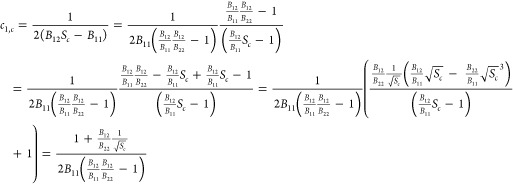
As a result, the original three co-existence eqs 15–17 are now replaced by four equations (eqs 49–50). The solutions of eqs 49–50 can be expressed in terms of the so-called Lambert-W function,³⁹ previously already invoked to solve the symmetrical case where B₁₁ = B₂₂,³¹ as

51

where, for the remainder of this paper, the (arbitrary) convention is used that the “lower right” phase with c₁^I > c_1,s and c₂ < c_2,s is labeled I and the “upper left” phase with c₁^II < c_1,s and c₂ > c_2,s is labeled II, in line with Figure 1. This convention can be used because the co-existing phases (c₁^I, c₂) and (c₁^II, c₂) should always be in diagonally opposite quadrants relative to the point (c_1,s, c_2,s). Substitution of eq 51 in eq 48 leads to

52

Equation 37 becomes in this notation

53

Progress has been made by parametrization of the problem, where the original four-variable problem (c₁^I, c₂, c₁^II, c₂) has been effectively reduced to a two-variable problem ((c₁^I, c₂) in eq 52), where S_m acts as a parameter that has to be chosen in the interval [S_c,S_∞] or [S_∞,S_c], depending on whether S_c or S_∞ is smaller. Here, S_∞ is the absolute value of the slope of the tie-line in molar units far away from the critical point, as demonstrated in the Appendix VII section (cf. eq 115 in Dewi et al.³¹)

54

Once (c₁^I, c₂) is determined for a certain S_m, the values for (c₁^II, c₂) can be determined analytically from eq 51. Note that in the symmetrical case, where S_m = 1 for all tie-lines, the solution is given directly in Dewi et al.³¹ Care has to be taken that the correct branch of the Lambert-W function is chosen, W_–1 or W₀, as indicated in eqs 51 and 52. In addition, the parametrization of the problem reveals the symmetry properties of the equations that are hidden in the initial co-existence equations. These symmetry properties allow us to find explicit solutions for specific cases, but these expressions in eq 52 still have to be solved numerically in the general case to find the properties of the phase diagram. It should also be emphasized that eq 52 is invariant under the transformation (c₁^I, c₂, S_m) ↔ (c₂^II, c₁, 1/S_m). Table 1 summarizes the values for (c_1,s, c_2,s) in three well-defined limits of S_m. Note that the matrix in eq 52 simplifies in the symmetrical case, where B₁₁ = B₂₂ ≡ B, S_m = 1, and , and eq 48 reduces to

55

Table 1. Values for (c_1,s, c_2s) in Three Well-Defined Limits of S_m.

Sm = Sc	Sm

leading to diagonalization of the matrix

56

Substitution of eq 56 in eqs 49–50 leads to the analytical result for the binodal that was previously reported for the symmetrical case as³¹

57

58

where (c_1,bi, c_2,bi) represent the coordinates of the binodal.

Although other formal limits exist in which the matrix in eq 52 diagonalizes as

59

(when c₁ and/or c₂ → ∞, or when B₁₂ → ∞ for a fixed critical point), both limits are unphysical in the sense that they describe situations in which the total equivalent hard-sphere volume fraction φ = (B₁₁c₁ + B₂₂c₂)/4 is vastly larger than O(1). Since the maximum packing for hard spheres is about 0.7, depending on the details, it is reasonable to expect that (B₁₁c₁ + B₂₂c₂)/4 should not exceed a value of O(1) by many orders in other cases. Therefore, the cases for these formal limits are not addressed here, except for a short note on the behavior of the slope of the tie-lines in one of these limits in the next section.

Degeneracy in the Virial Coefficients for the Critical Point

Consider two sets of virial coefficients that give rise to the same critical point, (B₁₁, B₁₂, B₂₂) and (B₁₁^*, B₁₂, B₂₂^*). Using eq 28, an expression for S_∞ can be obtained

60

and

61

When B₁₂ ≠ B₁₂^*, it follows that S_∞ ≠ S_∞, which means that the tie-lines far away from the critical point are generally not parallel to each other for two sets of virial coefficients that give rise to the same critical point. However, numerical evidence shows that the changes in the slope of the tie-lines tend to be modest over most of the range of B₁₂. This is quantified below.

From eqs 26 and 27 and the requirement that (B₁₁, B₂₂) > 0, a bound on B₁₂, can be directly derived as

62

Using the following expressions that were derived from eqs 24 and 25

63

the slope of the tie-line far away from the critical point, −S_∞, can be written as

64

or

65

For large B₁₂, the above equation can be expanded in a Taylor series to linear order as

66

From eq 66, it follows that S_∞ → S_c for B₁₂ → ∞ and S_∞/S_c – 1 decays proportionally to 1/B₁₂ for large B₁₂. S_∞/S_c varies only in a relatively narrow range of B₁₂ close to the value where one of the pair B₁₁ and B₂₂ becomes zero. The phase separation criterion behaves for large B₁₂ as

67

Therefore, as B₁₂ increases to large values, the phase separation criterion reaches its critical value of 1, edging closer and closer to stability.

Figure 3 shows the behavior of eqs 66 and 67 for a specific choice of virial coefficients.

Figure 3.

(Solid line) |S_∞/S_c–1| and (dashed-dotted line) as a function of B₁₂ for a fixed critical point with c_1,c = 2.0521 mol/m³, c_2,c = 0.0445 mol/m³, and S_c = 0.0777; (dotted line) limits for large B₁₂ according to eqs 66 and 67; and (red solid circle) |S_∞/S_c–1| for the systems for which the phase diagrams are described in Figure 6.

Degeneracy in the Virial Coefficients for a Single Tie-Line

In case the composition of the co-existing phases is known, but none of the virial coefficients is known, an infinite number of solutions is found for the virial coefficients. It can be shown (the Appendix VIII section) that the same tie-line (or co-existing phases) is obtained for two triplets of virial coefficients (B₁₁, B₁₂, B₂₂) and (B₁₁^′, B₁₂, B₂₂^′), provided

68

(which is similar to eq 28). This corresponds to a line in B-space that can be written in vector notation as

69

with λ₂ being any real number, ensuring that and all B’s are larger than zero. A support vector can be found by choosing an arbitrary real value for B₁₁ (i.e., B₁₁ = 1) from which B₁₂ and B₂₂ can be calculated from eqs 35 and 36.

Removing Degeneracy in Virial Coefficients Using More Than One Experimental Result: Intersection of the Lines in B-Space

In the previous sections, it was shown that a single data point (like the critical point or a tie-line) is insufficient to determine a unique set of virial coefficients. There is always a line in B-space that satisfies the requirements for one of these requirements. Next, the use of two data points (a critical point and a tie-line or two tie-lines) to obtain a unique set is discussed. It is shown that this approach is possible in theory, as it involves finding the intersection of two nonparallel lines in B-space, but it requires an experimental accuracy that is not likely to be achieved in practice. The case where the critical point and one of the tie-lines are known is considered below, but the example can easily be adapted for the case where two tie-lines are known.

First, consider a phase diagram that is characterized by a set of virial coefficients (B₁₁, B₁₂, B₂₂). As the discussion in the previous sections has shown, each critical point (cf. eq 29) or tie-line (cf. eq 69) in the diagram can be represented by triplets of virial coefficients situated on lines in B-space. These lines fan out from a single point in B-space that corresponds with the actual virial coefficients (B₁₁, B₁₂, B₂₂). In theory, no more than two lines in B-space are needed to determine the actual triplet (B₁₁, B₁₂, B₂₂).

Next, consider the inverse case: two sets of virial coefficients that satisfy the individual requirements for a critical point and a tie-line are known and are points on lines in B-space that give rise to the same critical point or tie-line. The intersection of the two lines of individual solutions, P_c and P_t, is the common solution and can be found from

70

71

From the discussion above, it can be concluded that in the nonsymmetrical case (B₁₁ ≠ B₂₂), in theory, two tie-lines or a tie-line and a critical point can be used to determine a unique set of virial coefficients. In practice, however, the range over which S_m varies is small and the experimental inaccuracy in the determination of the composition of the co-existing phases is too high to exploit this approach.

Sensitivity of the Shape of the Phase Diagram to the Choice of the Virial Coefficients in Degenerate Cases

Above, it was established that in the general case it is possible to have an infinite number of combinations of virial coefficients that give rise to the same feature in a phase diagram (a critical point, a tie-line). It was also established that two features (the critical point + a tie-line, two tie-lines) fix the choice of the virial coefficients and therefore the phase diagram. For the special symmetric case (B₁₁ = B₂₂), a single feature is sufficient to fix the choice of the virial coefficients.

What was not established is whether the phase diagram in the first case (virial coefficients based on a single feature) is sensitive to the choice of a triplet (B₁₁, B₁₂, B₂₂) on the corresponding line in B-space. Numerical calculations are presented below to address this question. The near-symmetrical and asymmetrical cases are distinguished.

Near-Symmetrical Cases

In near-symmetrical cases, where B₁₁ ≈ B₂₂, the binodal is almost mirror-symmetrical relative to the line c₁ = c₂. This is illustrated in Figure 4, where the phase diagrams are calculated for the different sets of virial coefficients (B₁₁, B₁₂, B₂₂) = (4, 3, 1) (m³/mol) and (B₁₁, B₁₂, B₂₂) = (1, 3, 4) (m³/mol). Figure 4 shows that the binodals nearly superimpose, although the tie-lines and spinodals are distinctly different. It is noted that the spinodal is sensitive to the choice of the virial coefficients, as was to be expected from the expressions for their asymptotic values (see discussion below eq 33).

Figure 4.

(Red solid line) Binodal A for (B₁₁, B₁₂, B₂₂) = (4, 3, 1) (m³/mol) corresponding to critical point A and binodal B for (B₁₁, B₁₂, B₂₂) = (1, 3, 4) (m³/mol) corresponding to critical point B. Critical point B is mirror-symmetrical to critical point A relative to the line c₁ = c₂. Binodal C for (B₁₁, B₁₂, B₂₂) = (1, 1.948, 1) (m³/mol) corresponds to the critical point located on the line c₁ = c₂ intersecting binodal A. It shows that binodal A, B, and C are nearly mirror-symmetrical relative to the line c₁ = c₂ and superimpose within the numerical error. Note that for binodals A, B, and C, the ratio B₁₁/B₂₂ is 4, 1/4, and 1, respectively. The corresponding spinodals ((blue dashed line) labeled A, B, and C) and tie-lines ((dashed-dotted line) labeled A, B, and C) are distinctly different from each other.

In near-symmetrical cases, it is possible to find a binodal for a symmetric case, where B₁₁ = B₂₂, that nearly overlaps the original binodal; in this example, B₁₁ = B₂₂ = 1 (m³/mol), B₂₂ = 1.948 (m³/mol) was used. The method to determine the virial coefficients to find the corresponding symmetrical binodal is described in the Appendix IX section (eq 144).

Clearly Asymmetrical Cases

Typically, B₁₁ and B₂₂ differ substantially (B₁₁ ≪ B₂₂ or B₁₁ ≫ B₂₂) and the binodal becomes asymmetric. Even though each point on the binodal can be interpreted as a new critical point for a different set of virial coefficients (cf. Appendix X), the binodals through this new critical point generally do not superimpose on the binodal of the original critical point. This is illustrated in Figure 5.

Figure 5.

Binodal A and critical point A corresponding to (B₁₁, B₁₂, B₂₂) = (1.54, 4.00, 5.85) (m³/mol). Binodal B and critical point B corresponding to (B₁₁, B₁₂, B₂₂) = (1.00, 16.00, 194.71) (m³/mol). Here, the critical point B is selected on binodal A. It shows that binodal A and binodal B do not superimpose. Note that for binodal A, we have B₁₁/B₂₂ = 0.263 and for binodal B, we have B₁₁/B₂₂ = 0.005. The spinodals (blue dashed line), binodals (red solid line), and tie-lines (dashed-dotted line) corresponding to critical points A and B (solid circle) are indicated by labels A and B.

Focusing on binodals for the same critical point, but different virial coefficient combinations (cf. Figure 3), it was shown that S_c is the same (Appendix V). Triplets of virial coefficients that lead to the same critical point do not lead to the same slope of the tie-lines far away from the critical point, −S_∞ = −√(B₁₁/B₂₂). As a result, triplets of virial coefficients that lead to the same critical point do not lead to the same phase diagram. In practice, S_∞ only varies significantly if either B₁₁ or B₂₂ get very close to zero. When B₁₂ → ∞, we find that the binodal converges to the analytical expression given in eq 66. It is noted that when B₁₂ → ∞, all tie-lines become parallel to each other with a slope −S_c and the phase diagrams for a fixed critical point converge to the same phase diagram for B₁₂ → ∞. This is illustrated in Figure 6. Three phase diagrams are shown for the virial coefficient triplets. Label A: (B₁₁, B₁₂, B₂₂) = (0.0052, 3.2000, 29.9146) (m³/mol), label B: (B₁₁, B₁₂, B₂₂) = (1.00, 16.00, 194.71) (m³/mol), and label C: (B₁₁, B₁₂, B₂₂) = (5.9774, 80, 1017.5) (m³/mol). These parameter combinations share the same critical point (c_1,c, c_2,c) = (2.0521, 0.0445) (mol/m³). The spinodals are sensitive to the choice of the virial coefficients. The spinodal and tie-lines B and C nearly superimpose, whereas A and B are clearly different. The same is true for the binodals, although the differences are smaller. One could question whether any of the differences would be sufficiently large to be discerned experimentally. Also, the tie-lines are sensitive to the choice of the virial coefficients. The slope −S_∞ = −√(B₁₁/B₂₂) of the tie-lines increases when moving away from the critical point (binodal A: S_∞ = 0.013; binodal B: S_∞ = 0.071; binodal C: S_∞ = 0.274).

Figure 6.

Binodal A corresponds to (B₁₁, B₁₂, B₂₂) = (0.0052, 3.2000, 29.9146) (m³/mol). Binodal B corresponds to (B₁₁, B₁₂, B₂₂) = (1.00, 16.00, 194.71) (m³/mol). Binodal C corresponds to (B₁₁, B₁₂, B₂₂) = (5.9774, 80, 1017.5) (m³/mol). All three binodals have the same critical point (solid circle) located at (c_1,c, c_2,c) = (2.0521, 0.0445) (mol/m³). It shows that binodal A does not superimpose with binodal B or C. The binodals B and C do superimpose for all practical purposes and their tie-lines are very close. The spinodals (blue dashed line), binodals (red solid line), and tie-lines (dashed-dotted line) are indicated by labels A, B, and C. These systems are also indicated in Figure 3, which plotted |S_∞/S_c – 1| for tie-lines far away from the critical point.

Conclusions

This paper investigated the solutions of the Edmond–Ogston model, a virial model that takes into account virial coefficients up to the second order and which can be used to describe phase separation in binary mixtures of polymers in a common solvent. The real strength of this model is for relatively low polymer concentrations. The model becomes more qualitative when the polymer concentrations exceed the overlap concentrations and a description of the polymer blend in terms of single polymer particles with pair interactions starts to fail and other models to describe the physics of polymer mixtures should be introduced. While some results for the Edmond–Ogston model, in particular, the expression for the critical point, were obtained previously in a normalized form,^31,32 the present analysis is done in experimentally accessible coordinates like molar concentrations.

A parametrization is introduced that essentially allows for an evaluation of the composition of the co-existing phases at constant osmotic pressure in a natural way. The parameterization simplifies the analysis and reduces the calculation effectively from a four-variable problem into a two-variable problem. Moreover, the parameterization reveals the symmetry of the mathematical structure of the equations and the pivotal role that is played by the so-called Lambert-W functions. The reformulation of the problem also reveals why an exact solution to the problem can be given for the symmetrical case (B₁₁ = B₂₂).

Furthermore, the present formulation of the problem revealed that individual properties of the phase diagram (e.g., the critical point or tie-line) are described by an infinite number of triplets (B₁₁, B₁₂, B₂₂) of virial coefficients. The properties of these triplets were investigated and were found to be represented by straight lines in “B-space”. If the features of the phase diagram are determined with infinite precision, two properties of the phase diagram (e.g., two tie-lines, one tie-line plus a critical point) suffice to determine the actual virial coefficients. In practice, the data is not accurate enough to achieve this, echoing an observation previously made by Clark.²⁹

It is found that nearly any choice of virial coefficients gives rise to the same critical point and a similar phase diagram. The binodal and tie-lines for all of these choices almost superimpose, making it unlikely that one could distinguish between the calculated binodals experimentally. The calculated spinodals do depend on the choices of virial coefficients but are experimentally less accessible. Only for choices where B₁₁ or B₂₂ nearly vanish (before they become negative), meaningful differences are observed between phase diagrams.

It was also established that every point on the binodal can be considered as a critical point for another choice of virial coefficients. However, generally, the binodals through these critical points do not superimpose, except if the values of B₁₁ and B₂₂ are close, leading to a nearly symmetrical binodal.

Although the present paper focused on the Edmond–Ogston model, the observations should essentially hold for the Flory–Huggins model too, given the equivalence between both models up to the second order of the expansion in the concentrations as identified by Clark.²⁹

The present paper also provides a procedure to calculate the various properties of the phase diagram, in particular the tie-lines. The critical point and spinodal can be calculated analytically through eqs 24, 25, and 33. The present results indicate that the best method to calculate the properties of the binodal and tie-lines involves the following steps

• Calculate the minimum and maximum slope of the tie-lines, −S_c, and −S_∞ using eqs 22, 23, and 54 (note that S_c is not necessarily smaller than S_∞)

• Choose the slope −S_m of an intermediate tie-line having a value between −S_c and −S_∞

• Calculate c_1,s and c_2,s using eq 42

• Solve matrix eq 52 for c₁^I and c₂

• Determine c₁^II and c₂ by means of eq 51

From a practical point of view, the present results indicate that although the two coordinates for the critical point are insufficient to determine the model parameters accurately, they are sufficient to determine most features of the phase diagram with fair accuracy. The shape of the binodal seems to be least sensitive to the choice of the virial coefficients in the Edmond–Ogston model. The slope of the tie-lines shows variations only in a relatively narrow range of values for B₁₂. The spinodal is the most sensitive to the choice of the three virial coefficients.

The obtained results reveal the intricacies of the Edmond–Ogston model, especially in the context of degeneracies within the model. This deeper understanding of the model helps to assess the possibilities and limitations of the use of phase diagrams from the literature to extract virial coefficients and in this way build a database of parameters to describe the phase behavior of many polymer mixtures.

Appendices

Appendix I: Comparison of the Flory–Huggins and (Extended) Edmond–Ogston Models for Binary Polymer Mixtures in a Solvent

The aim of this appendix is to compare the Flory–Huggins model to the (extended) Edmond–Ogston model. The extension includes the third-order terms in concentration because issues with the Flory–Huggins model arise there. Symbols not explained in this appendix have the same meaning as in the main text.

Starting from the expression for the Helmholtz free energy (cf. eq 1)

72

where C₁₁₁, C₁₁₂, C₁₂₂, and C₂₂₂ are the third-order virial coefficients, leads to the following equations for the extended Edmond–Ogston model

73

74

75

For the Flory–Huggins model, the notation of Clark was used,²⁹ except that the subscripts have been changed and the solvent is referred to as component 0 and both polymers as components 1 and 2; furthermore, Δ in the expressions for Δμ_i was dropped

76

77

78

Here, p₁ and p₂ are the molecular weights of polymers 1 and 2; χ₁₀ and χ₂₀ are the Flory–Huggins interaction parameters between polymers and solvent and χ₁₂ between both polymers; and φ₀, φ₁, and φ₂ are the volume fractions of the solvent and both polymers.

The osmotic pressure in the Flory–Huggins model can be obtained from eq 76 and using the substitution

79

which leads to (cf. eq 10)

80

Expansion of φ₀ around 1 (because the total polymer concentration can be considered small) using

81

and truncating to the third order results in

82

The chemical potential for polymer 1 in the Flory–Huggins model can be obtained from eq 77 as

83

A similar relation for polymer 2 can be obtained from eq 78 as

84

It is now possible to match the parameters in both models. The results are summarized in Table 2.

Table 2. Matching of Terms between Flory–Huggins and Extended Edmond–Ogston Models.

extended Edmond–Ogston model parameters	Flory–Huggins model parameters, from eq 76	Flory–Huggins model parameters, from eq 77	Flory–Huggins model parameters, from eq 78
c1
c2
B11	υs(1 – 2χ10)p12
B22	υs(1 – 2χ20)p22
B12
C111
C112
C122
C222

To match the equations for the osmotic pressure and the chemical potentials in the Flory–Huggins model consistently up to the second order, one has to make the (reasonable) assumption that 1/p₁ ≪ 1 – 2χ₁₀ and 1/p₂ ≪ 1 – 2χ₂₀. The absolute value of the chemical potentials is shifted by a constant, but this does not matter as the differences between the chemical potentials in two phases are compared, and the chemical potentials are shifted in each phase by the same value.

To ensure that the coefficients are consistent up to the third order, one has to assume that χ₁₀ = χ₂₀ = χ₁₂ = υ_s. This is a problem because this fixes all of the adjustable parameters in the Flory–Huggins model. In addition, it is surprising that the third-order parameters in eqs 77 and 78 in the Flory–Huggins model are expressed in terms of the binary interaction parameters.

The Maxwell relation (cf. eq 6) reflects that the Helmholtz free energy is a state variable. This relation is fulfilled for the extended Edmond–Ogston model, which can be demonstrated using eqs 74 and 75

85

For the Flory–Huggins model, however, it is found that

86

and

87

From eqs 86 and 87, the validity of the Maxwell relation requires that

88

which is only valid in special cases (e.g., when the properties of polymer 1 are indistinguishable from those of polymer 2). Therefore, in general, the Maxwell relation does not seem to hold for the Flory–Huggins model.

Appendix II: The Gibbs Phase Rule for a Mixture of N Components Distributed in F Phases

(A) For the chemical potentials, we find from thermodynamic equilibrium requirements that

89

This gives N(F – 1) equations with NF unknowns.

(B) For the osmotic pressures, we find from thermodynamic equilibrium requirements that

90

This gives (F – 1) equations.

We find from A and B a total of (N + 1)(F – 1) equations and NF unknowns. The number of equations can never be greater than the number of unknowns, from which it follows that

91

or F ≤ N + 1. The degree of freedom D is introduced as

92

When N = 2 and F = 2, it follows that D = 1, which implies that one of the concentrations can be varied to find the binodal.

When N = 2 and F = 3, it follows that D = 0, which implies that there can be a three-phase equilibrium for a binary mixture, but it corresponds to a point (or points) in the phase diagram since D = 0.

Appendix III: The Expressions for the Critical Point (Equations 24 and25) Are Equivalent to the Expressions Used in Dewi et al.³¹

Here, it is demonstrated that

93

can be written in the form used for the critical point by rewriting the expressions for the requirement for the critical point, eqs 20 and 21 (or eq A.8 in Dewi et al.³¹), as

94

95

respectively. In this case

96

and

97

or in the notation of our previous paper³¹

98

99

where α = B₁₂/B₁₁, β = B₁₂/B₂₂, and S_c = √(β/α)·s_c. Note that the slope at the critical point in normalized units, −s_c, was written with a capital −S_c in our previous paper.³¹

Appendix IV: The Third-Order Stability Polynomial (Equation 20 or21) Is Equivalent to the Edmond–Ogston Expression Involving the Critical Point

Equation 20 can be rewritten as

100

or

101

Equation 101 can be substituted in the rather convoluted identities for (2B₁₂S_c)³ and (2B₁₂/S_c)³

102

103

Since the critical point is given by (cf. eqs 24 and 25)

104

105

Equations 104 and 105 can be rewritten as eq 5a,b in Edmond and Ogston²⁸

106

107

introducing the notation of Edmond and Ogston²⁸ for the virial coefficients

108

109

110

By ultimately taking the cube root, the desired result is obtained

111

112

(where the indices in the notation of Edmond and Ogston²⁸ were changed to the present convention, (2,3) → (1,2)). Therefore, it can be concluded that eq 5a,b in Edmond and Ogston²⁸ is an alternative representation of eq 20, the third-order polynomial defining the critical point.

Appendix V: If Two Triplets of Virial Coefficients Give Rise to the Same Critical Point, They Also Give Rise to the Same Slope for the Binodal and Spinodal at the Critical Point

To define a valid critical point using an alternative set of virial coefficients (B₁₁^*, B₁₂, B₂₂^*), this set needs to satisfy eq 20

113

From

114

it follows that

115

116

or

117

The original set of virial coefficients satisfies the third-order polynomial (with S_c not changed), therefore

118

The term B₁₂^* – B₁₂ can be divided, leading to

119

which is true and proves the assertion.

Appendix VI: Demonstration on How Equations 49 and 50 Follow from Equations 16 and 17

Starting from eq 16, the terms in B₁₂ can be moved to the same side of the equation. Applying the definition of S_m from eq 45 leads to

120

Placing all terms for phase I on one side and those for phase II on the other side leads to

121

Using the definition for c_1,s in eq 42 and subtracting a term ln(c_1,s) on both sides, this can be written in the form of eq 49. Similarly, it is possible to rewrite eq 17 as

122

yielding eq 50.

Appendix VII: The Value of S_m at the Critical Point and Far Away from the Critical Point

Here, the values of the slope −S_m are given in two limits. First, the case close to the critical point is addressed, where the following expression can be written by substitution of eqs 24 and 25

123

From this, it can be concluded that S_m equals S_c in this limit. Second, the case far away from the critical point is addressed, where c₁^I ≫ c₁ and c₂^II ≫ c₂ (assuming without loss of generality that phase I can be found at the bottom-right and phase II at the top-left compared to the critical point). Equation 39 for the slope of the tie-line far away from the critical point, −S_∞, can now be rewritten as

124

From this, it follows that

125

or

126

or

127

Appendix VIII: If Two Sets of Virial Coefficients Give the Same Slope of the Tie-Line, They Also Give the Same Co-existing Phases

For an alternative set of virial coefficients (B₁₁^′, B₁₂, B₂₂^′) to result in the same co-existing phases, the new virial coefficients need to satisfy the equivalent of eqs 15–17

128

129

130

Using a similar approach as previously for the critical point (cf. eqs 115 and 116)

131

132

So

133

134

135

The original equations for the set (B₁₁, B₁₂, B₂₂) can be subtracted now

136

137

138

In eqs 136–138, (B₁₂^′ – B₁₂) can be divided and the following equations are obtained after rearranging

139

140

141

Each of the eqs 139–141 can be rewritten in the form of eq 45. A similar observation can be made here as for the critical point: from the form of the coordinates in eq 42, it can be concluded that if all virial coefficients B_ij are multiplied by the same factor k, the coordinates in eq 42 are divided by a factor k. In contrast to the situation for the critical point, however, the slope −S_m changes because not every term in the right-hand side of eq 39 for S_m features is a virial coefficient.

Appendix IX: The Intersection of a Binodal with the Line c₁ = c₂

The critical point (c_1,c, c_2,c) is given by eqs 24–25 or 104–105. A critical point for the symmetrical case (C_s, C_s) can always be expressed as

142

Equations 57 and 58 provide an analytical expression for the binodal in the symmetrical case through the critical point. Substituting (C_s, C_S) for the critical point belonging to the symmetrical binodal and (c_1,c, c_2,c) for the nonsymmetrical point that should be placed on the symmetrical binodal, the following expression is obtained

143

Substituting the explicit expressions for (c_1,c, c_2,c, C_s), eqs 104, 105, and 142 result in

144

Equation 144 allows for the determination of B₁₂^• – B^• since (B₁₁, B₁₂, B₂₂) are known. B₁₂ – B^• specifies a line in B-space resulting in the same (symmetrical) critical point, similar to eq 28.

Appendix X: Any Point on the Binodal Can Be Written as a Critical Point for a Different Triplet of Virial Coefficients

Points on the binodal can be expressed as

145

and the critical point for a different set of virial coefficients can be represented as

146

If the actual point in the phase diagram is the same, the following equation can be obtained

147

148

where the terms (B₁₂^′S_m – B₁₁), (B₁₂^*S_c – B₁₁), , and are constant within the sets (B₁₁^*, B₁₂, B₂₂^*) and (B₁₁, B₁₂^′, B₂₂). This leads to

149

150

The left-hand side can be interpreted as the set of virial coefficients (B₁₁^*, B₁₂, B₂₂^*) that map on the same critical point (cf. Appendix V), whereas the right-hand side can be interpreted as the set of virial coefficients (B₁₁, B₁₂^′, B₂₂) that map on the same point on the binodal (cf. the Appendix VIII section). The equation expresses the relation between the virial coefficients if one wants to switch the role of a point from being just on the binodal to being a critical point. A consequence of the existence of this relation is that any point on the binodal can also be a critical point if an alternative set of virial coefficients is chosen.

The authors declare no competing financial interest.

References

- Semenova M. G.Equilibrium in Colloidal Systems. In Thermodynamics of Phase Equilibria in Food Engineering; Gambini Pereira C., Ed.; Academic Press: Cambridge, MA, 2018; Chapter 12, pp 507–528. [Google Scholar]
- Hu W.Polymer Phase Separation. Polymer Physics; Springer: Vienna, 2012; pp 167–185. [Google Scholar]
- Cheng S. Z. D.Metastable States in Phase Transitions of Polymers. Phase Transitions in Polymers—The Role of Metastable States; Elsevier, 2008; Chapter 4, pp 77–155. [Google Scholar]
- Frith W. J. Mixed biopolymer aqueous solutions - phase behaviour and rheology. Adv. Colloid Interface Sci. 2010, 161, 48–60. 10.1016/j.cis.2009.08.001. [DOI] [PubMed] [Google Scholar]
- Levelt-Sengers J.How Fluids Unmix. Discoveries by the School of Van der Waals and Kamerlingh Onnes. History of Science and Scholarship in the Netherlands; Koninklijke Nederlandse Akademie van Wetenschappen: Amsterdam, 2002; Vol. 4. [Google Scholar]
- Norton I. T.; Frith W. J. Microstructure design in mixed biopolymer composites. Food Hydrocolloids 2001, 15, 543–553. 10.1016/S0268-005X(01)00062-5. [DOI] [Google Scholar]
- Doublier J. L.; Garnier C.; Renard D.; Sanchez C. Protein-polysaccharide interactions. Curr. Opin. Colloid Interface Sci. 2000, 5, 202–214. 10.1016/S1359-0294(00)00054-6. [DOI] [Google Scholar]
- Tolstoguzov V. B. Functional properties of food proteins and role of protein-polysaccharide interaction. Food Hydrocolloids 1991, 4, 429–468. 10.1016/S0268-005X(09)80196-3. [DOI] [Google Scholar]
- Tombs M. P.; Peacocke A. R.. The Osmotic Pressure of Biological Macromolecules; Clarendon Press: Oxford, U.K., 1974. [Google Scholar]
- Cui K.; Nan Ye Y.; Lin Sun T.; Yu C.; Li X.; Kurokawa T.; Ping Gong J. Phase separation behavior in tough and self-healing polyampholyte hydrogels. Macromolecules 2020, 53, 5116–5126. 10.1021/acs.macromol.0c00577. [DOI] [Google Scholar]
- Minton A. P. Simple calculation of phase diagrams for liquid-liquid phase separation in solutions of two macromolecular solute species. J. Phys. Chem. B 2020, 124, 2363–2370. 10.1021/acs.jpcb.0c00402. [DOI] [PMC free article] [PubMed] [Google Scholar]
- Wang F.; Altschuh P.; Ratke L.; Zhang H.; Selzer M.; Nestler B. Progress report on phase separation in polymer solutions. Adv. Mater. 2019, 31, 1806733 10.1002/adma.201806733. [DOI] [PubMed] [Google Scholar]
- Shi W.; Weitz D. A. Polymer phase separation in a microcapsule shell. Macromolecules 2017, 50, 7681–7686. 10.1021/acs.macromol.7b01272. [DOI] [Google Scholar]
- Philippe A. M.; Cipelletti L.; Larobina D. Mucus as an arrested phase separation gel. Macromolecules 2017, 50, 8221–8230. 10.1021/acs.macromol.7b00842. [DOI] [Google Scholar]
- Xia Y.; Friend R. H. Controlled phase separation of polyfluorene blends via inkjet printing. Macromolecules 2005, 38, 6466–6471. 10.1021/ma0503413. [DOI] [Google Scholar]
- Edelman M. W.; van der Linden E.; Tromp R. H. Phase separation of aqueous mixtures of poly(ethylene oxide) and dextran. Macromolecules 2003, 36, 7783–7790. 10.1021/ma0341622. [DOI] [Google Scholar]
- Lorén N.; Hermansson A. M.; Williams M. A. K.; Lundin L.; Foster T. J.; Hubbard C. D.; Clark A. H.; Norton I. T.; Bergström E. T.; Goodall D. M. Phase separation induced by conformational ordering of gelatin in gelatin/maltodextrin mixtures. Macromolecules 2001, 34, 289–297. 10.1021/ma0013051. [DOI] [Google Scholar]
- Choi J. M.; Holehouse A. S.; Pappu R. V. Physical principles underlying the complex biology of intracellular phase transitions. Annu. Rev. Biophys. 2020, 49, 107–133. 10.1146/annurev-biophys-121219-081629. [DOI] [PMC free article] [PubMed] [Google Scholar]
- Lee I. H.; Imanaka M. Y.; Modahl E. H.; Torres-Ocampo A. P. Lipid raft phase modulation by membrane-anchored proteins with inherent phase separation properties. ACS Omega 2019, 4, 6551–6559. 10.1021/acsomega.9b00327. [DOI] [PMC free article] [PubMed] [Google Scholar]
- Alberti S.; Dormann D. Liquid-liquid phase separation in disease. Annu. Rev. Genet. 2019, 53, 171–194. 10.1146/annurev-genet-112618-043527. [DOI] [PubMed] [Google Scholar]
- Hyman A. A.; Weber C. A.; Jülicher F. Liquid-liquid phase separation in biology. Annu. Rev. Cell Dev. Biol. 2014, 30, 39–58. 10.1146/annurev-cellbio-100913-013325. [DOI] [PubMed] [Google Scholar]
- Chronakis I. S.; Kasapis S. Preparation and analysis of water continuous very low fat spreads. LWT—Food Sci. Technol. 1995, 28, 488–494. 10.1006/fstl.1995.0082. [DOI] [Google Scholar]
- Bot A.; Foster T. J.; Lundin L. Modelling acidified emulsion gels as Matryoshka composites: Firmness and syneresis. Food Hydrocolloids 2014, 34, 88–97. 10.1016/j.foodhyd.2012.12.013. [DOI] [Google Scholar]
- Dekkers B. L.; Hamoen R.; Boom R. M.; van der Goot A. J. Understanding fiber formation in a concentrated soy protein isolate - pectin blend. J. Food Eng. 2018, 222, 84–92. 10.1016/j.jfoodeng.2017.11.014. [DOI] [Google Scholar]
- Schaink H. M.; Smit J. A. M. Protein–polysaccharide interactions: The determination of the osmotic second virial coefficients in aqueous solutions of β-lactoglobulin and dextran. Food Hydrocolloids 2007, 21, 1389–1396. 10.1016/j.foodhyd.2006.10.019. [DOI] [Google Scholar]
- Touchet T. J.; Cosgriff-Hernandez E. M.. Hierarchal Structure–Property Relationships of Segmented Polyurethanes. In Advances in Polyurethane Biomaterials; Cooper S. L.; Guan J., Eds.; Woodhead Publishing: Cambridge, U.K., 2016; Chapter 1, pp 3–22. [Google Scholar]
- Flory P. J.Principles of Polymer Physics; Cornell University Press: Ithaca, NY, 1953. [Google Scholar]
- Edmond E.; Ogston A. G. An approach to the study of phase separation in ternary aqueous systems. Biochem. J. 1968, 109, 569–576. 10.1042/bj1090569. [DOI] [PMC free article] [PubMed] [Google Scholar]
- Clark A. H. Direct analysis of experimental tie-line data (two polymer – one solvent system) using Flory-Huggins theory. Carbohydr. Polym. 2000, 42, 337–351. 10.1016/S0144-8617(99)00180-0. [DOI] [Google Scholar]
- Ersch C.; van der Linden E.; Martin A.; Venema P. Interactions in protein mixtures. Part II: A virial approach to predict phase behaviour. Food Hydrocolloids 2016, 52, 991–1002. 10.1016/j.foodhyd.2015.07.021. [DOI] [Google Scholar]
- Dewi B. P. C.; van der Linden E.; Bot A.; Venema P. Second order virial coefficients from phase diagrams. Food Hydrocolloids 2020, 101, 105546 10.1016/j.foodhyd.2019.105546. [DOI] [Google Scholar]
- Dewi B. P. C.; van der Linden E.; Bot A.; Venema P. Corrigendum to “second order virial coefficients from phase diagrams”. Food Hydrocolloids 2021, 112, 106324 10.1016/j.foodhyd.2020.106324. [DOI] [Google Scholar]
- Berne B. J.; Pecora R.. Dynamic Light Scattering; Wiley: New York, 1976; pp 173–174. [Google Scholar]
- Mächtle W.; Börger L.. Analytical Ultracentrifugation of Polymers and Nanoparticles; Springer: Heidelberg, 2006. [Google Scholar]
- Reichl L. E.A Modern Course in Statistical Physics; Edward Arnold: London, 1980. [Google Scholar]
- McMillan W. G.; Mayer J. E. The statistical mechanics of multicomponent systems. J. Chem. Phys. 1945, 13, 276–305. 10.1063/1.1724036. [DOI] [Google Scholar]
- Grinberg V. Y.; Tolstoguzov V. B. Thermodynamic incompatibility of proteins and polysaccharides in solutions. Food Hydrocolloids 1997, 11, 145–158. 10.1016/S0268-005X(97)80022-7. [DOI] [Google Scholar]
- Ermakova A.; Anikeev V. I. Calculation of spinodal line and critical point of a mixture. Theor. Found. Chem. Eng. 2000, 34, 51–58. 10.1007/BF02757464. [DOI] [Google Scholar]
- Corless R. M.; Gonnet G. H.; Hare D. E. G.; Jeffrey D. J.; Knuth D. E. On the Lambert W function. Adv. Comput. Math. 1996, 5, 329–359. 10.1007/BF02124750. [DOI] [Google Scholar]