High‐Resolution Agent‐Based Modeling of COVID‐19 Spreading in a Small Town

Abstract

Amid the ongoing COVID‐19 pandemic, public health authorities and the general population are striving to achieve a balance between safety and normalcy. Ever changing conditions call for the development of theory and simulation tools to finely describe multiple strata of society while supporting the evaluation of “what‐if” scenarios. Particularly important is to assess the effectiveness of potential testing approaches and vaccination strategies. Here, an agent‐based modeling platform is proposed to simulate the spreading of COVID‐19 in small towns and cities, with a single‐individual resolution. The platform is validated on real data from New Rochelle, NY—one of the first outbreaks registered in the United States. Supported by expert knowledge and informed by reported data, the model incorporates detailed elements of the spreading within a statistically realistic population. Along with pertinent functionality such as testing, treatment, and vaccination options, the model accounts for the burden of other illnesses with symptoms similar to COVID‐19. Unique to the model is the possibility to explore different testing approaches—in hospitals or drive‐through facilities—and vaccination strategies that could prioritize vulnerable groups. Decision‐making by public authorities could benefit from the model, for its fine‐grain resolution, open‐source nature, and wide range of features.

A high‐resolution agent‐based model is proposed to reproduce COVID‐19 spreading in small towns and cities. The model encapsulates many real‐world features including disease transmission in residential and public locations, different testing approaches, treatments, and interventions. The model accuracy and potentialities are demonstrated on real data from New Rochelle, NY, and through “what‐if” analyses of targeted vaccination campaigns.

1. Introduction

In December 2019, COVID‐19 was first observed in humans in Wuhan, the Hubei Province's capital in China. The World Health Organization (WHO) declared this outbreak as a Public Health Emergency of International Concern on January 30, 2020, and later named it a pandemic on March 11, 2020. As of December 23, 2020, the WHO has reported 76 382 044 cases globally, with 1 702 128 deaths.^{[ 1 ]} In the United States, the number of infected individuals keeps rising, with tens of thousands of newly infected cases discovered every day. The Centers for Disease Control and Prevention (CDC) has reported 17 974 303 cases as of November 23, 2020.^{[ 2 ]} Following an unprecedented containment campaign based on lockdowns, most countries seek a delicate balance between safety and normalcy, aiming for a safe return to normal activities amidst less restrictive conditions.

Timely case detection through efficient testing and contact tracing is among the key components required for lowering the COVID‐19 spread before a vaccine becomes available.^{[ 3} , ⁴ , ⁵ , ^{6 ]} Important questions on testing pertain to the identification of infected individuals and their contacts. Addressing these questions calls for an improved understanding of community structure, outbreak locations, and individual lifestyles.^{[ 7} , ^{8 ]} Due to the scale of the COVID‐19 epidemic, an additional burden has been placed on traditional testing sites, such as hospitals, emergency rooms, and walk‐in clinics, thereby challenging their safety.^{[ 9} , ¹⁰ , ^{11 ]}

Computational models are powerful tools for understanding novel epidemics and evaluating the effectiveness of potential countermeasures.^{[ 12} , ¹³ , ¹⁴ , ¹⁵ , ^{16 ]} Agent‐based models (ABMs) are a class of computational models that provide a high‐resolution—both temporal and spatial—representation of the epidemic at the individual level.^{[ 4} , ¹⁷ , ¹⁸ , ¹⁹ , ²⁰ , ^{21 ]} These models afford consideration of multiple physical locations, such as businesses or schools, as well as unique features of communities, like human behavioral trends or local mobility patterns.

Once validated, ABMs can be used to test competing “what‐if” scenarios that would otherwise require impractical and, potentially, unethical experiments. For example, Ferguson et al. developed an ABM to investigate the impact of non‐pharmaceutical interventions for COVID‐19, such as nation‐wide confinement in the United Kingdom and the United States.^{[ 22 ]} Aleta et al. proposed an ABM for the entire Boston metropolitan area to elucidate the role of different types of contact tracing measures in maintaining low levels of infection.^{[ 4 ]} Gressman and Peck created an ABM of a university campus to examine strategies for the safe reopening of higher education institutions.^{[ 23 ]} Hinch et al. formulated an open‐source agent‐based modeling framework to support the analysis of select non‐pharmaceutical interventions and contact tracing schemes.^{[ 24 ]} The merits of ABMs have been recognized by a large number of studies, which have shed light on technical aspects of their implementation as well as their scalability across scenarios.^{[ 25} , ²⁶ , ²⁷ , ²⁸ , ^{29 ]}

The focus of existing ABMs is either small micro‐environments or entire countries and large metropolitan areas, where the population is purposefully coarsened to enable numerical simulation. Medium‐size and highly resolved communities constitute an important, yet unconsidered, modeling scale for COVID‐19. America is a “nation of small towns,” as described by the US Census,^{[ 30 ]} and after the initial wave of spreading in the New York metropolitan area, we see that small and medium‐size towns are increasingly hit by the pandemic. A high‐resolution ABM can closely capture real‐world communities and interaction patterns at this intermediate scale, thereby allowing them to carefully reflect town‐specific lifestyles without requiring coarsening to perform massive simulation campaigns. Thus, the synthetic generation of a one‐to‐one virtual population with its own individual buildings (residential and public) opens a wide range of new possibilities in epidemiological analysis, which may inform public health authorities to design accurate and targeted interventions. The analysis could include lockdowns of different parts of the town and afford to quantify the effect of testing practices, treatment prevalence, and vaccination strategies.

Toward the study of these medium‐size populations, we develop an agent‐based modeling platform of COVID‐19 for the entire town of New Rochelle, located in Westchester County in New York. This location was chosen as it was one of the earliest COVID‐19 outbreaks in the United States and is representative of a typical small town. The ABM replicates, geographically and demographically, the town structure obtained from the US Census statistics.^{[ 31 ]} The model is based on the earlier ABM developed by Ferguson's research group to study pandemic influenza,^{[ 19} , ²⁰ , ^{21 ]} which has been recently adapted to study COVID‐19.^{[ 22 ]} The proposed ABM expands the original model by Ferguson et al.^{[ 19} , ²⁰ , ^{21 ]} along several directions. First, we incorporate two testing strategies: traditional, in‐hospital testing with a non‐negligible risk of infection, and a “safe” drive‐through testing.^{[ 32} , ³³ , ³⁴ , ^{35 ]} Second, we account for temporal variations in time‐dependent testing capacity to reflect the change in resource allocation during the course of the pandemic. Third, our model explicitly includes multiple COVID‐19 treatment types, such as home isolation, hospitalization, and hospitalization in intensive care units (ICUs). Fourth, we separately track individuals with COVID‐19‐like symptoms due to other diseases like seasonal influenza or the common cold. These individuals are expected to play an important role in the epidemic by imposing an additional burden on testing resources. Fifth, we individually model employees in schools, hospitals, and retirement homes, enabling a dedicated consideration of these professions. Finally, the model permits the selective study of important interventions, such as business and school closures and their reopening and vaccination strategies. After validation against real data, we explore alternative “what‐if” vaccination scenarios, which may be relevant in the next several months. We consider a foreseeable situation in which a limited number of vaccines will be available. In addition to random vaccination, we explore the possibility of prioritizing vaccination for groups of individuals whose status or profession makes them particularly vulnerable to COVID‐19 infection: healthcare, school, and retirement home workers, as well as residents. Along with selective vaccination of hospital employees, we assess the potential benefit of schools and businesses' concurrent closures.

2. The Database of New Rochelle, NY

2.1. Geography and population data sources

We collected and organized a database of geographical coordinates, type, capacity, residential buildings, and public spaces in the town of New Rochelle, NY. The database was created by manually collecting geographical coordinates and characteristics of each residential and public building in the town using OpenStreetMap^{[ 36 ]} and Google Maps.^{[ 37 ]} The database and the code for creating the town and its population are available through our repository (https://github.com/Dynamical‐Systems‐Laboratory/NR‐ABM‐population). The population data were collected in March and April 2020 from US Census using 2018 5‐year average tables for New Rochelle.^{[ 31 ]} Since then, some of the data changed slightly, and the reader is referred to our repository for the exact datasets. Data regarding the number of students and employees in local schools was obtained from the National Center of Education Statistics,^{[ 38 ]} while the hospital staff and patient number estimates were based on the records from the New York State Department of Health^{[ 39 ]} and the American Hospital Directory.^{[ 40 ]} Figure  1 shows the locations considered in the model.

Figure 1.

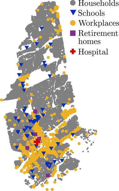
Map of New Rochelle, NY, which highlights the residential and public buildings included in the database.

2.2. Household, Schools, and Workplace Assignment of Agents

Households were assigned to agents using Census data on household and family structure, vacancy rate, and the number of sub‐units and floors in multi‐unit buildings. Figure  2a) shows the population distribution of the model set at the start of the simulation (see Section S3, Supporting Information), which mirrors the increased density registered toward the southern part of the town.^{[ 41 ]} As demonstrated in Figure 2b), the distribution of household sizes and the mean size is in good agreement with Census data. As evidenced in Figure 2c,d, we closely match the distribution of employed family members and the overall age distribution, accurately resolving several age groups. As reported in Table  1 , we are successful in maintaining similar percentages of households with agents who are above 60 years old. This aspect is particularly important for realistic predictions of COVID‐19, which is significantly more severe and fatal among the older population. Aside from age, the modeled community preserves the ratio of families with children and of single‐parent households, as shown in Table 1.

Figure 2.

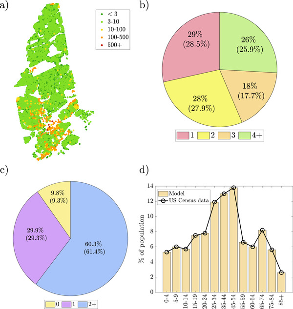
Select characteristics of the created (virtual) households: a) sizes of residential buildings across town; b) percentage of households of a given size (census data in brackets); c) distribution of employed members per family (census data in brackets); and d) age distribution of the population.

Table 1.

Modeled properties of the population and US Census data for New Rochelle, NY

Category	Model	US Census value
Mean household size	2.77	2.71
Households with one or more individuals 60 years and older	47.0%	42.3%
Families with children	39.1%	34.2%
Single parent families	18.7%	25.0%

This article is being made freely available through PubMed Central as part of the COVID-19 public health emergency response. It can be used for unrestricted research re-use and analysis in any form or by any means with acknowledgement of the original source, for the duration of the public health emergency.

All children aged 5–17 were assigned to schools of appropriate levels. The number of students in a school was proportional to school size based on the data from the National Center for Education Statistics.^{[ 38 ]} Accordingly, the initial distribution of students in the model, representing time before the pandemic, was set so that a portion of children younger than 5 years old was placed in daycare, and similarly, 35% of individuals between 18 and 21 years old attended the town's higher education institutions.

A portion of agents older than 16 were allowed to work and study according to a set of rules based on the estimated workplace and school sizes (see Section S3, Supporting Information). Agents' workplace distribution was generated using the US Census data on the percentage of the population working in a given industry while the number of employees at hospitals, schools, and retirement homes was estimated. The initial numbers of retirement homes residents were estimated based on institution size. The initial number of hospital patients with a condition other than COVID‐19 was set to occupy one‐sixth of the total available beds. The exact steps for creating the population from building information and census data are outlined in Section S3, Supporting Information.

2.3. COVID‐19 Data Sources

The number of total and active New Rochelle cases were collected manually from official reports and videos available for Westchester County.^{[ 42 ]} The mortality and testing statistics were obtained from the Official Twitter account of the Westchester County,^{[ 42 ]} and the New York State Department of Health,^{[ 43 ]} respectively, for Westchester County as a whole, and were then scaled to the population of New Rochelle. All the data are available through our repository (https://github.com/Dynamical‐Systems‐Laboratory/NR‐ABM‐population).

3. COVID‐19 ABM with Testing and Treatment

3.1. Model Overview

During a day, agents transition between different locations (identified in the New Rochelle database: households, workplaces, schools, retirement homes, and hospitals). In each of these locations, they can interact with other agents, thereby supporting the transmission of COVID‐19. Agents can be healthy, undergoing testing, or be under treatment. We assume that the town is isolated, such that the agents cannot leave the town, and new agents cannot enter during the simulation.

Motivated by refs. [19, 20, 22], the COVID‐19 progression model consists of five states: susceptible (S), exposed—which includes infectious individuals who have not yet developed symptoms—(E), infectious‐symptomatic ($Sy$), removed‐healed (R), and removed‐dead (D); with a detailed outline of states, their variants, and transitions as shown in Figure  3 . Upon infection, susceptible agents become exposed (E) and remain so for a latency period. Following the COVID‐19 infectiousness profile, we assume that exposed agents are not infectious during the initial part of the latency period. When the latency period is over, exposed agents develop symptoms and become infectious‐symptomatic ($Sy$).^{[ 4 ]} Some exposed agents may recover without ever developing symptoms (that is, they are asymptomatic); in this case, their latency period is extended to match the expected COVID‐19 recovery period.

Figure 3.

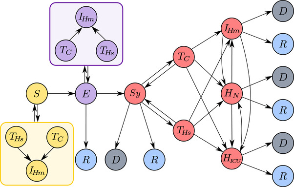
Schematic representation of modeled agent states and their possible transitions. Agent in the model can be in one of the following states: susceptible (S); exposed (E); symptomatic ($Sy$); removed ‐ dead (D); removed ‐ healthy/recovered (R); Agents in different states can undergo testing in a test car ($T_C$), or a hospital ($T_{Hs}$) after which they can be treated through home isolation ($I_{Hm}$), normal hospitalization ($H_N$), or hospitalization in an intensive care unit, ICU ($H_{ICU}$). In addition to symptomatic agents, exposed agents and agents who have COVID‐19‐like symptoms but are not infected can also be tested. Except for the symptomatic agents, all positive test results, including false positives, will lead to home isolation.

Exposed agents and agents showing symptoms —whether from COVID‐19 or another condition— have the possibility of being tested which can be performed either in a hospital ($T_{Hs}$) or a car ($T_C$). Testing in a hospital carries the possibility of infecting hospital staff and patients with a condition other than COVID‐19. Additionally, if the agent is COVID‐19‐negative, then the agent is at risk of becoming infected during testing. We assume that drive‐through testing does not carry the risk of infection based on the work of Upham.^{[ 34 ]} The outcomes of a test can be true positive or negative or false positive or negative.

After testing, agents are assigned treatment from one of the following three treatment types: home isolation ($I_{Hm}$), routine hospitalization ($H_N$), and hospitalization in an ICU ($H_{ICU}$). An exposed agent who has tested positive for COVID‐19 will always undergo home isolation until developing symptoms, at which point their treatment can potentially change to $H_N$ or $H_{ICU}$. In contrast, a symptomatic agent can be assigned to one of the three treatments. A symptomatic agent can transition between different treatment types during the course of the disease. All infected agents are removed through either recovery (R) or death (D). A removed agent no longer contributes to the spread of the infection.

A symptomatic agent who is untested will not undergo treatment, and their removal is determined following similar rules to the tested agents. However, an untested agent requiring ICU treatment has an increased probability of dying, to account for the higher mortality in the absence of a diagnosis. While the agents undergoing testing are routinely quarantined, those who are not deemed to be tested retain their normal activities. However, when developing symptoms, these agents will refrain from going to work or school, thereby reducing the contribution to contagion in public areas.

Susceptible agents can have symptoms similar to COVID‐19 due to non‐COVID‐19 diseases, such as a common cold or seasonal influenza.^{[ 44 ]} We assume that this population is constant throughout the duration of the simulation. Since these susceptible agents are suspected of having COVID‐19, they can undergo testing and thus introduce two additional elements in our model: i) they increase the count of people being tested, and therefore the burden on testing sites, and ii) they can contract COVID‐19 upon interacting with infected people at the testing site. Finally, such agents can be erroneously tested positive during their recovery from the non‐COVID‐19 disease. However, after recovery, these agents are still susceptible to COVID‐19.

To simulate realistic COVID‐19 epidemic conditions, we introduce school closures, a state‐wide lockdown, and the three reopening phases I, II, and III. School closure is modeled by omitting the contribution of schools to the transmission of COVID‐19. Similarly, lockdown and reopening phases are characterized by tuning the contributions of the workplaces to the transmission. The number of tests performed per day can be time‐dependent, following real practices.^{[ 43 ]}

3.2. COVID‐19 Transmission Dynamics

The proposed epidemiological model consists of COVID‐19 transmission through agents interacting at their residences and public places. The agents reside in households, retirement homes, or hospitals when being treated for conditions other than COVID‐19. They can also attend schools and go to work; employees of schools, retirement homes, and hospitals are modeled explicitly for their high‐risk and critical role. Following the original work of Ferguson, there is no distinction between times of the day, for example day versus night. At each simulation step, $\mathrm{\Delta }t$, an agent may contract the disease or infect other agents at home, school, workplace, or hospital.^{[ 19} , ^{20 ]} For example, if a susceptible agent is a high school student who also works part‐time, their probability of being infected with COVID‐19 is computed based on their contacts at their school, workplace, and household. When agents are being tested or hospitalized, they do not infect those in their households, schools, or workplaces.

The model comprises a set of agents $\mathcal{N}=\{1,\dots ,n\}$ and a set of locations $\mathcal{L}=\{1,\dots ,L\}$. According to the town database, an agent is associated with a subset of locations determined by the model input. Formally, we define a set of functions $f_q:\mathcal{N}\to \mathcal{L}$, with $q\in \{\mathrm{H},\mathrm{W},\mathrm{S},\mathrm{Rh},\mathrm{Hsp}\}$, so that function $f_q$ associates each agent $i\in \mathcal{V}$ to the corresponding location $\ell \in \mathcal{L}$ of type q. The types of locations are households (H), workplaces (W), schools (S), retirement homes (Rh), and hospitals (Hsp). Note that each agent may not be associated to all the types of locations. To denote that agent i is not associated to a location of type q, we write $f_q(i)=\varnothing$. We denote by $n_{\ell }$ the number of agents associated with location ℓ.

At every simulation step (of duration $\mathrm{\Delta }t$), infected agents assigned to location ℓ contribute to the probability of infection for susceptible agents at that location. Specifically, the probability that an agent i that is susceptible at time t becomes infected in the following time‐step is equal to

$$p_i(t):=1-e^{-\mathrm{\Delta }t{\mathrm{\Lambda }}_i\left(t\right)}$$ (1)

where the non‐negative time‐varying parameter ${\mathrm{\Lambda }}_i(t)$ quantifies the contagion risk at all the locations associated with the agent and it is equal to

$$\begin{array}{c}\hfill \begin{array}{c}\hfill {\mathrm{\Lambda }}_i\left(t\right):={\lambda }_{\mathrm{H},f_{\mathrm{H}}(i)}\left(t\right)+{\lambda }_{\mathrm{W},f_{\mathrm{W}}(i)}\left(t\right)+{\lambda }_{\mathrm{S},f_{\mathrm{S}}i}\left(t\right)+{\lambda }_{\mathrm{Rh},f_{\mathrm{Rh}}(i)}\left(t\right)+{\lambda }_{\mathrm{Hsp},f_{\mathrm{Hsp}}(i)}\left(t\right)\end{array}\end{array}$$ (2)

where each contribution represents the so‐called infectiousness function of each type of location associated with agent i, with the understanding that ${\lambda }_{q,\varnothing }=0$, that is, if agent i is not associated with any location of type q, than locations of type q do not contribute to the agent's contagion risk.

The infectiousness function of a location ℓ of type q at time t, ${\lambda }_{q,\ell }(t)$, due to all the agents (indexed by k) at that location, is defined as

$$\begin{array}{c}\hfill {\lambda }_{q,\ell }\left(t\right):=\frac{1}{n_{\ell }^{{\alpha }_q}}\sum _{k=1}^{n_{\ell }}\left(E_k{\rho }_k{\beta }_{q,k}+S{y}_k{\psi }_{\ell }{c}_k{\rho }_k{\beta }_{q,k}\right)\end{array}$$ (3)

The sum is performed over the $n_{\ell }$ agents who are associated with location ℓ and it represents a weighted ratio between the number of exposed and infected agents and all the agents at the location; $E_k$ is an indicator function that is equal to 1 if agent k is in the exposed (E) and has become infectious and 0 otherwise; $S{y}_k$ is equal to 1 if agent k is symptomatic ($Sy$) and 0 otherwise. The parameter ${\rho }_k\ge 0$ models variability in infectiousness among the agents; $c_k>1$ is a factor that measures the increased infectiousness of a symptomatic agent compared to an exposed one; ${\alpha }_q\le 1$ is a size scaling parameter (less than one for households and one otherwise); ${\psi }_{\ell }\in [0,1]$ is an absenteeism correction for workplaces and schools, which is used to model reduction of agent presence upon developing symptoms; ${\beta }_{q,k}\ge 0$ is a transmission rate that generally depends on the type of location q and on the activity of agent k at that particular location (e.g., the transmission rate for an agent who is being tested at a hospital is different from an agent who works there). Further details of the model are provided in Section S1, Supporting Information.

When an agent becomes exposed, they undergo an incubation period. The latency of the incubation is drawn from a log‐normal distribution, which allows for the possibility of some agents to not spread the virus until they develop symptoms. Once the incubation ends, an agent transitions from exposed to symptomatic. The model allows for a portion of exposed agents to recover without symptoms (commonly referred to as asymptomatic individuals) by including their recovery time within their incubation period.

3.3. Testing

Both exposed and symptomatic agents can undergo testing for COVID‐19 according to two different probabilities. When an agent is scheduled to be tested, they are placed under home isolation and randomly assigned to a testing location—a drive‐through or a hospital. We assume that the test is performed for a fixed amount of time after the decision to be tested, and similarly that the result of a test appears after a fixed delay following the test. The test result can be either positive (true or false) or negative (true or false), with negative results causing the agent to return from home isolation to the community. An exposed agent confirmed positive for COVID‐19 remains in home isolation, while a symptomatic one is given an initial treatment.

Testing is performed differently for exposed hospital employees and patients originally admitted for non‐COVID‐19‐related diagnosis (such as a car accident or cancer treatment). These agents do not undergo home isolation, and their testing is always performed in the hospitals they work or reside in, without the option of a test car. The symptomatic hospital staff is home isolated prior to receiving the test results, while the non‐COVID‐19 patients stay in the hospital and, upon developing COVID‐19 symptoms, they are counted among hospitalized COVID‐19 cases. This fine level of detail is needed to capture evidence of extensive COVID‐19 spreading in the early stage of the pandemic in hospitals.^{[ 45} , ⁴⁶ , ^{47 ]} After confirming COVID‐19, agents are assigned treatment.

With the exception of hospital employees and patients who develop disease symptoms, the model does not apply any explicit contact tracing. Instead, case detection is implemented in an average sense. Whether an agent will be tested is determined by stochastic sampling of a uniform distribution, followed by a comparison with testing prevalence at that time.

3.4. Treatment

When a symptomatic agent is confirmed COVID‐19 positive, they are assigned to one of the three formal treatments according to a probabilistic mechanism: home isolation, regular hospitalization, and hospitalization in an ICU.^{[ 22} , ^{24 ]} Afterward, the agent can change treatment types depending on their recovery status and clinically observed COVID‐19 progression. The agent's initial treatment is chosen based on the probability of normal hospitalization and hospitalization in an ICU obtained from clinical data depending on their age.^{[ 22} , ^{48 ]} In both cases, agents are assigned to a random hospital. If hospitalized in an ICU, their recovery status is recomputed based on an agent's probability of dying in an ICU.^{[ 22 ]} All other agents are placed in home isolation.

Treatment changes include all possible transfers except direct transfer from an ICU to home isolation, as outlined in Figure 3. In our model, whether an agent dies or recovers is determined upfront when the agent develops symptoms of the disease. Treatment transitions are closely related to an agent's future recovery outlooks. An agent originally determined to die and treated in an ICU will die in the ICU.^{[ 49 ]} Upon recovering, agents will be transferred to normal hospitalization after an amount of time decided a priori.^{[ 22 ]} Any dying agent who was previously confirmed COVID‐19 positive would be placed in an ICU for a predetermined number of days before death.^{[ 50 ]} A recovering agent initially hospitalized outside an ICU can become home isolated if their recovery time exceeds their hospital stay.^{[ 49 ]} Finally, an agent recovering while isolated at home can become hospitalized for a certain amount of time, a commonly observed course for the disease.^{[ 49} , ^{51 ]}

3.5. Initialization and Vaccination

At the beginning of the simulation, we initialize the entire population as susceptible, assuming no prior immunity in a virtually COVID‐19‐free population. Then, a predefined number of agents are assigned the exposed health state. These agents can only be tested after developing symptoms.

Part of the susceptible population can also be vaccinated and thus becomes immune. The vaccines are distributed by two modes: i) randomly throughout the entire population, or ii) to a specific type of agent, such as healthcare workers or retirement home employees.

3.6. Agent Removal

Disease progression can have two possible outcomes: recovery or death. The outcome is determined using age‐based mortality data, the agent's treatment requirements, and current testing prevalence. An agent's mortality also depends on whether they are tested and receive proper medical attention.^{[ 50} , ⁵² , ⁵³ , ⁵⁴ , ^{55 ]} Specifically, while asymptomatic agents always recover, we distinguish between two events that can occur to symptomatic agents and influence their probability of dying.

The model decides if an agent needs ICU care upon exhibiting symptoms. An agent who needs an ICU will be admitted upon being tested. Not all the agents who need an ICU will be admitted to one; those who are not tested, and therefore not diagnosed, will die. Among the agents who do not need an ICU, a fraction may still die, for example, due to heart failure, stroke, or a rapid decline in condition; some of these individuals will die in their homes, but some others will formally be admitted to ICU, despite not needing it, based on the agent's expected lifetime.

All these probabilities are available from empirical observations except the probability of dying without the need of an ICU. In order to estimate this quantity, we perform the following calculations. We expand the overall probability that a symptomatic agent dies, $P(D|Sy)$, using the law of total probability with respect to the conditioning on whether the symptomatic agent needs ICU treatment, N, and the event that the symptomatic agent does not need an ICU, $\overline{N}$,

$$P(D|Sy)=P(D|N)P(N)+P(D|\overline{N})P(\overline{N})$$ (4)

By rearranging Equation (4), we obtain the following closed‐form expression for the required probability

$$P(D|\overline{N})=\frac{P(D|Sy)-P(D|N)P(N)}{1-P(N)}$$ (5)

In the following, we derive the three expressions for $P(D|Sy)$, $P(D|N)$, and $P(N)$, which are needed to compute the formula.

First, the probability of dying for symptomatic agents, $P(D|Sy)$, is inferred from the infection fatality ratio ($IFR$) available in the literature.^{[ 22 ]} Since the $IFR$ is based on serology‐informed estimations, it reflects the probability of dying for an infected agents (regardless of whether the agent is symptomatic or not). Assuming that asymptomatic agents do not die, we can compute the overall time‐averaged probability that a symptomatic agent dies by re‐scaling the $IFR$ by the probability of developing symptoms once contracting COVID‐19, $P(Sy|\mathrm{CoV})$, obtaining

$$P(D|Sy)=\frac{IFR}{P(Sy|\mathrm{CoV})}$$ (6)

Second, the probability of dying if an agent needs an ICU, $P(D|N)$, in Equation (5) is computed depending on whether they are tested once they become symptomatic. Specifically, by means of the law of total probability with respect to the conditioning on the event T, we have

$$P\left(D|N\right)=1-\left(1-P(D|N,T)\right)P\left(T|Sy\right)$$ (7)

where $P(T|Sy)$ is the probability that a symptomatic agent is tested. Since the $IFR$ used in Equation 6 is a temporal average over the entire duration of the pandemic, the probability $P(T|Sy)$ is also estimated as an average over the entire duration of the pandemic, from data reported in Table S9, Supporting Information.

Third, the probability that a symptomatic agent needs ICU care, $P(N)$, is computed from empirical data on the probability that an agent needs to be hospitalized, $P(H)$, and the probability that symptomatic hospitalized agents need ICU care, $P(N|H)$, yielding

$$P(N)=P(N|H)P(H)$$ (8)

where these empirical data are reported in Table S7, Supporting Information.

Finally, the required probability is computed by substituting Equations (6)–(8) into Equation (5).

When an agent dies, they are removed from all public places, hospitals, or current residences. Recovered agents become active in public locations, and if hospitalized, return to their households or retirement homes. Recovered agents who were previously hospitalized for a condition other than COVID‐19 are readmitted to the hospital.

3.7. Susceptible Agents with COVID‐19‐Like Symptoms

Susceptible agents with COVID‐19‐like symptoms do not exist in the model until the onset of testing. Once testing efforts begin, these agents are assigned as a fraction of those who are still susceptible. A portion of these agents will undergo testing and receive either a false positive or a true negative result. Therefore, the probability of a susceptible agent with COVID‐19‐like symptoms to be tested, $p(T,Sy,\overline{\mathrm{CoV}})$, is given as

$$\begin{array}{c}\hfill p(T,Sy,\overline{\mathrm{CoV}})=\left(p\left(\mathrm{true}\mathrm{negative}|Sy\right)+p\left(\mathrm{false}\mathrm{positive}|Sy\right)\right)p(T)\end{array}$$ (9)

We assume that the probability of getting a false negative among COVID‐19‐infected symptomatic agents when the epidemic prevalence is low is negligible.^{[ 56} , ^{57 ]} We can then approximate the probability of a true negative by the probability of receiving a negative result.

If scheduled to be tested, the agent is assigned a test time and a testing site (either a randomly chosen hospital or a drive‐through test). When the test occurs, the time is selected from a Gamma distribution to avoid these agents undergoing home isolation and testing simultaneously. Similar to the procedure for an infected agent undergoing testing, the agent displaying COVID‐19‐like symptoms is placed under home isolation for a certain amount of time before testing occurs. Home isolation lasts until the agent is confirmed negative or reaching “recovery” after a false‐positive result. The duration of the home isolation before the test and the subsequent wait time for results is the same for these agents as for the infected ones.

If an agent with COVID‐19‐like symptoms contracts COVID‐19, they become an exposed agent. To maintain a fixed fraction of such agents in the population, a new susceptible agent is then randomly chosen to take their place, provided such agents are still present in the population.

3.8. Lockdown and Reopening Events

Our model provides options to simulate school closure, lockdown, and three reopening phases, 1, 2, and 3. School closures are simulated by zeroing the transmission rates of students and employees. The business closure and reopening are implemented through user‐defined reduction or increase of the initial workplace transmission rates, respectively. The model also allows for adjusting the absenteeism correction of a workplace, that is, ${\psi }_{\ell }$ in Equation (3), to a lockdown value, valid through the reopening phases. The transmission parameters for households, hospitals, and retirement homes remain unchanged throughout the simulation.

3.9. Model Parameters

Parameters originate from several sources: established literature data used in other ABMs,^{[ 19} , ²⁰ , ²¹ , ^{22 ]} clinical data on COVID‐19,^{[ 22} , ⁴⁹ , ⁵¹ , ^{58 ]} and information from a clinical consultant who is part of the team. In addition, due to the lack of concrete data, some of our parameters are informed estimates, in line with the current understanding of COVID‐19 from scientific literature and the media. Furthermore, some parameter types are identified from reported data through model calibration. These latter parameters are the number of initially infected agents, time‐varying testing prevalence, COVID‐19 transmission changes following closures and reopening phases, and asymptomatic agents' age distribution. Parameters, data sources, and assumptions are listed and indicated in Section S2, Supporting Information.

There are four groups of model parameters: COVID‐19 transmission dynamics parameters, testing parameters, parameters related to closure and reopening events, and other parameters, all listed as Tables in the Supporting Information. Transmission dynamics originates from the COVID‐19 agent‐based model in Ferguson et al.^{[ 22 ]} While not explicitly stated, the transmission dynamics parameters used therein mirror those previously developed for influenza by the same research group. Such a choice is justified since COVID‐19 is a respiratory disease that spreads^{[ 19} , ^{20 ]} similarly to influenza. However, to make the transmission rates more representative, we further scale them by the ratio of reproductive numbers, R ₀, for these two diseases. R ₀ represents the average number of secondary infections directly caused by a single infected individual.^{[ 59 ]} Following analogous models and procedures, R ₀ for COVID‐19 was estimated to be 2.4,^{[ 22 ]} while for influenza it was reported as $R_0=1.7$, resulting in a scaling factor of 1.41.^{[ 20 ]}

Hospital‐related transmission rates are calculated by scaling equivalent non‐hospital rates with data from our clinical consultant in Italy. Specifically, we use the fact that there was a 7.2% increase in infection among hospital employees in a given week in Italy compared to a 3.7% increase in the general population. Thus, we use a ratio of these percentages as our scaling factor to multiply a base rate of choice. The base rate for a hospital employee is the workplace rate, and for an agent hospitalized as a non‐COVID‐19 patient, it is the household rate. Other hospital rates are set relative to these following personal communication with the clinical consultant in Italy.

Hospitalization duration in the model is derived from the literature,^{[ 22 ]} and linearly scaled by a factor of 0.39 according to the data in the paper by Richardson et al.^{[ 49 ]} which are specific to the geographic region considered in this work. Specifically, the study by Richardson et al.^{[ 49 ]} provides actual hospitalization duration in New York City, though without distinguishing between ICU and non‐ICU treatment, and relative lengths of these two. Hence, we use the ratio of the total hospital treatment duration reported in Richardson et al.^{[ 49 ]} and Ferguson et al.^{[ 22 ]} to obtain locally realistic hospitalization periods.

4. Model Validation

To demonstrate our platform's viability, we simulated the spread of COVID‐19 from February 22 to July 14, 2020, from the onset of the epidemic to phase three of the reopening. In particular, this window includes the period in which all the schools in the town of New Rochelle were closed (March 13, 2020), followed by the restrictive state‐wide lockdown during which only essential businesses, such as grocery stores, were allowed to operate.

In our calibration, we used officially reported data on the total number of detected infections, number of people currently infected with the disease, and the total number of fatalities. From the cumulative number of cases and mortality, we extracted the number of new cases and deaths reported each week. To calibrate upon this dataset, we varied the initial number of infected agents, the percentage of tested population, the reduction in workplace transmission rates during the lockdown and its subsequent increase during the reopening periods, and age‐dependent fractions of asymptomatic agents as is summarized in Section S2, Supporting Information. Parameters were manually initialized, while the testing percentages were later refined using simplex optimization in MATLAB via the fminsearch function. Testing prevalence was set to vary with time, mimicking the actual testing practices in the region.^{[ 43 ]} In other words, the fraction of infected individuals who could be tested was time‐dependent. To match it, we used the data on newly confirmed cases every week during the simulation period, computed from total detected cases. We performed 100 realizations of the simulation, randomly selecting a fixed number of initially infected agents each time. All the parameters used in the simulations are listed in Section S2, Supporting Information. The computational performance of the model is summarized in Section S4, Supporting Information; the implementation is fairly efficient and approachable for general use, with 600 steps (150 days) of the simulation taking less than 30 s on a standard laptop.

Figures  4 and  5 show the results of the validation. Figure 4 compares the model output with real data along with five different metrics: i) the total number of cases, ii) the number of new cases, iii) the weekly average of active cases, iv) the total number of deaths, and v) the number of deaths in a week. The total number of cases was calculated as the number of agents who tested positive, including false positives and those who died without treatment. The number of new weekly cases was calculated as the weekly increase in the total number of cases. Working with weekly averages facilitates comparisons by filtering out spurious oscillations from uneven reporting and data collection by the authorities. In our model, the number of active cases was computed as the number of agents undergoing treatment confirmed positive or false positive. These were compared directly to the reported weekly average. The number of deaths includes both treated and undetected, untreated agents, assuming that COVID‐19 would be confirmed in individuals who have died, regardless of their testing status. The number of deaths per week was computed as the weekly rise in total fatalities.

Figure 4.

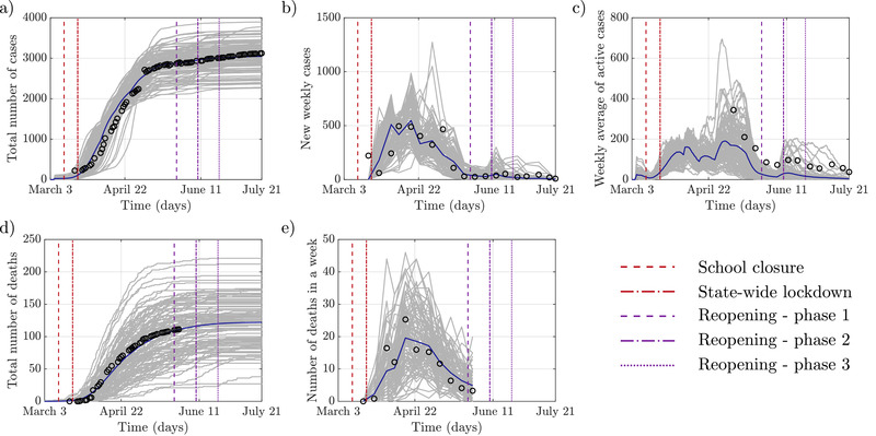
Comparison of the modeled COVID‐19 epidemic and officially reported data: a) The cumulative number of infections; b) New infections detected within a week; c) Active cases averaged over each week; d) The total number of deaths; e) Number of deaths in each week. The gray lines represent each of the simulation's 100 realizations, the blue line is the average value, and black circles are the reported data.

Figure 5.

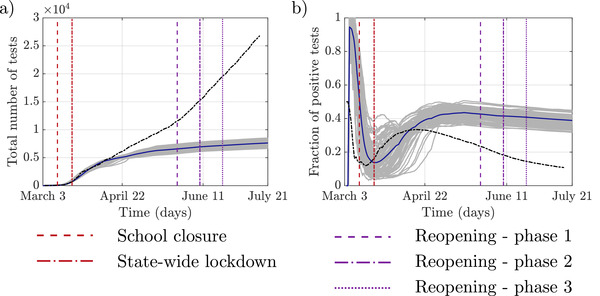
Comparison of modeled and reported testing practices: a) The total number of performed tests; b) Fraction of positive test results, including false positives: the gray lines represent each of 100 realizations of the simulation, the blue line is the average value, and dashed black line is the reported data.

A comparison of the total number of cases shows good agreement between the model and real data obtained from official outlets of Westchester County.^{[ 42 ]} Similarly, the number of new cases is well predicted by our model. Looking closely, however, the model has a smooth progression of the disease compared to a sudden high number of initial cases in the real data. We note that our model imparts a simplistic scenario of the testing practice, whereby an aggressive contact tracing followed the town's initial case detection.^{[ 60 ]} This likely resulted in a large difference in the number of initial cases in our model versus the real data. Simulating this particular scenario is currently outside the scope of our model.

In the case of weekly averages of active cases, the model reasonably matches real data trends. At the same time, the mean value predicted by the model is slightly lower than the reported values, likely due to longer recovery times of COVID‐19 patients than utilized in the model. We note that compared to the total number of reported cases, which provide information about new infections, the number of active cases also includes the process of recovery. Regarding the number of deaths, the reported values were obtained for the entire Westchester County and scaled down to New Rochelle, proportionally to its population. Here too, we find a close agreement between simulated and real data.

Figure 5 compares the total number of tests and positivity in our simulations with the available data from local testing practices. Similarly to the number of deaths, this data was reported at the county level and was scaled down to match the population of New Rochelle for a meaningful comparison. Our results indicate reasonable agreement in the early phases of the epidemic with discrepancies later on. The lower number of total tests in our model is due to the rule used for testing, which is based on the total number of exposed and symptomatic individuals. In contrast, in reality, testing was ramped up to include the general population. The only susceptible agents who can be tested in the model, in its present incarnation, are those exhibiting COVID‐19‐like symptoms. The fraction of these individuals is low and chosen upfront in the model. This trend is also visible in the positivity values, whereby we find an inflated positivity in our simulations by a factor of four compared to the real data, again due to limited testing in our model. This difference shows that negative testing outcomes do not affect the general number of cases, as evidenced by the model agreement on the number of cases and deaths.

Figure  6 shows the number of agents who were undergoing a given treatment type. The number of agents isolated at home comprised individuals who were waiting for a test or test results. The prevalence of each type of treatment qualitatively matches the general distribution of cases. Home isolated individuals constituted the bulk of infected agents, followed by hospitalized individuals, and finally, a few hospitalized in ICUs.

Figure 6.

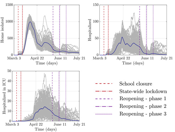
The number of agents undergoing each of the three treatment types at different time points in the simulation. The gray lines represent 100 realizations of the simulation; the blue line is the average value.

According to the New York State Department of Health, the New Rochelle hospital has 211 general and 12 ICU beds at its disposal under normal circumstances.^{[ 39 ]} In all realizations of our model, the number of hospitalized agents was always below the reported normal bed volume. In the model, the ICU demand was on average within standard hospital capacities, but in many simulations exceeded it two or even threefold. Given the expansion of hospital capacity as a response to COVID‐19^{[ 61 ]} and in the absence of reliable data, we consider this agreement reasonable.

5. Vaccination Study

To demonstrate the value of our platform, we performed a comparative analysis of different vaccination strategies. Specifically, we evaluated the effect of vaccinating only high‐risk groups of individuals, hospital, school, or retirement home employees, or retirement home residents and compare the results to a random immunization across the entire population.

The time period of this prospective study was aligned with the first wave of the epidemic, making the previously calibrated model the basis for the prediction. None of the parameters were changed in this study with respect to the earlier validation. The only differences in this vaccination study were the absence of school closures and any form of lockdown. In this context, the study also investigated the consequences of leaving schools and non‐essential businesses open throughout the first wave of the epidemic upon the availability of a vaccine.

Vaccination was implemented in the simulation on March 2^nd, simultaneously with the beginning of testing in New Rochelle. All the vaccines were distributed simultaneously, granting full protection against the disease. By then, some of the agents were already infected and were therefore excluded from vaccination. Susceptible agents with COVID‐19‐like symptoms were not vaccinated either, in an attempt to maintain an approximately fixed number of such agents in the simulation. We performed six sets of simulations with vaccinations of: i) hospital employees only, ii) school employees only, iii) retirement home employees only, iv) retirement home residents only, v) randomly selected fraction of the population, with the same size as the number of hospital employees, and vi) about a quarter of the town, corresponding to ten times the number of hospital employees.

Figure  7 shows the predictions from these six “what‐if” scenarios. The importance of closures is evident, with numbers of infections and fatalities exceeding reality many times. The vaccination of hospital employees resulted in only minor differences compared with the vaccination of an equivalent number of individuals among the general population. Similar observations can be made about targeted immunization of other vulnerable groups of agents. Significant differences only occur in mortality when vaccinating the elderly residents of retirement homes. Although both, targeted and random, approaches had some effect on COVID‐19 spread, massive immunization was the only truly impactful strategy. This finding is consistent with “herd immunity” predictions where effective containment of COVID‐19 can only be achieved with the large majority of the population acquiring immunity.^{[ 62 ]}

Figure 7.

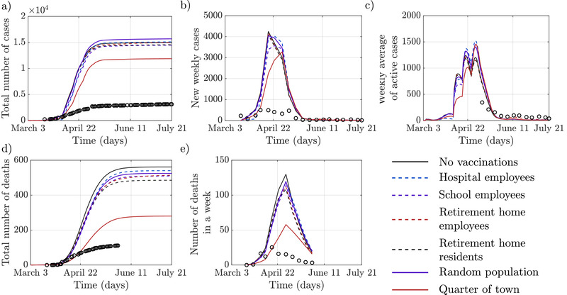
These figures show the spread of COVID‐19 epidemics across a range of “what‐if” scenarios, when no lockdowns or closures were set in place, and vaccinations were administered selectively. Only means are reported for visual clarity; also, officially reported data (black circles) are presented for reference. In the scenario where the only vaccinated agents were ones from specific high‐risk groups the vaccination covered on average 2,201 hospital employees (±11), 7577 school employees (±11), 494 retirement home employees (±2), and 1397 retirement home residents (±5).The number in parentheses indicates the standard deviation. In the fifth scenario, the number of people in the general population vaccinated was equivalent to the number of vaccinated hospital employees. A tenfold increase in the number of vaccinated individuals among the general population was considered in the third scenario.

6. Conclusions

Until widespread vaccination efforts are underway, maintaining a balance between safety and normalcy during the current COVID‐19 crisis requires the use of non‐pharmaceutical prevention measures as well as efficient detection strategies. The large number of testing strategies, unknowns, and high levels of uncertainties of this epidemic calls for the principled use of predictive computational models, potentially informing policy‐making with respect to widespread vaccination efforts.

In this work, we proposed a high‐resolution ABM of COVID‐19, developed for granular simulations of a small city or town, where each individual is explicitly modeled. We introduced several elements of novelty with respect to state of the art on ABM, including i) different testing strategies in hospitals and drive‐throughs; ii) time variations in testing prevalence; iii) multiple types of treatment, from home isolation to hospitalization in an ICU; iv) the presence of susceptible agents who have COVID‐19‐like symptoms due to other infections; v) explicit modeling of employees of hospitals, schools, and retirement homes; vi) school and business closures and reopenings; vii) comprehensive model calibration with officially reported data; and viii) incorporation of expert knowledge from the field.

We applied our model to the US town of New Rochelle, where one of the first COVID‐19 outbreaks in the country took place. Using an in‐house, detailed database of building locations, public and residential, and Census data, we created a geographically and statistically accurate representation of the town and its population. We demonstrated the possibility of accurately capturing the first wave of the COVID‐19 epidemic in the town.

As New Rochelle is a representative US small town, we believe that our validated model can serve as an analysis platform for numerous similar towns across the entire country, many currently facing the COVID‐19 crisis. To illustrate the model's value in analyzing prospective “what‐if” questions, we performed an immunization study in which we evaluated several vaccination strategies of future importance. In particular, we compared the impact of vaccination of select group of vulnerable individuals, including school employees, retirement home employees and residents, and the totality of the two thousand hospital employees in the town, a randomly selected group of 2000 individuals, and 20 000 randomly selected individuals out of the 80 000 people living in New Rochelle. Our results suggest that prioritizing vaccination of high‐risk individuals has a marginal effect on the count of COVID‐19 deaths. Predictably, a much more significant improvement is registered when a quarter of the town is vaccinated. Importantly, the benefits of the restrictive measures in place during the first wave greatly surpass those from any of these selective vaccination scenarios.

While undoubtedly useful, our model bears several limitations. First, the model lacks explicit agent mobility and random contacts, which manifest in a faster decline of the epidemic near the end of the simulation. The original model by Ferguson et al.^{[ 19} , ^{20 ]}, serving as the basis for our own, had an additional term to the model disease spreading through random contacts in the community. However, these contacts were based on commute and travel data at the level of the entire country, which is not directly applicable to the problem at hand of a small town. Simulating truly random interactions using a contact network approach similar to Hinch et al.^{[ 24 ]} may offer an alternative, which will be part of our future work. Along these lines, the impact of local travel and commute can further be included in the model by integrating traffic flow simulations.^{[ 63} , ⁶⁴ , ^{65 ]}

In addition to mobility and random contacts, our model does not include testing the general population, leading to possible under‐detection of cases in later reopening stages. While the model allows for testing uninfected individuals with symptoms, massive community testing is needed to align its outcomes with reality in later phases of the epidemic. Testing of general population along with random interactions is also expected to highlight the effects of different testing strategies already encoded within the model. Combined with contact tracing options, testing of general population is part of the next step in our platform's development.

Another limitation of our approach is in the modeling of hospitals in terms of their workforce and capacity. Specifically, we assume that infections of hospital employees do not trigger changes in the treatment of hospital patients and that hospitals have infinite beds and ICUs. Finally, we do not explicitly account for the use of personal protective equipment (PPEs), such as face coverings, and social distancing of agents. While these measures are included indirectly through reduction of disease transmission during the lock‐down and reopening phases, the ability of specific agents to protect themselves from the contagion would improve the granularity of the model and add a further realistic element, at the expenses of the computational burden. Advantageous impact of PPEs and distancing can be introduced to both susceptible and infected agents in a similar way to agent's current infectiousness variability, and this will be one of our goals in the nearest future.

Despite these limitations, our model matched real data very closely as the epidemic progressed through its initial stages. This correspondence allowed us to prospect and analyze alternative scenarios for COVID‐19, in which vaccination was accessible right at the onset of the first wave. Beyond the timely study of vaccination strategies, our model can be adapted to explore a range of pressing problems that are ahead of us by interested users who can directly modify our open‐source platform. For example, the model can be swiftly adapted to describe the concurrent spread of influenza with COVID‐19, which is expected to exacerbate the impact of second and third waves. Likewise, the model can provide clear and quantitative support to the long‐debated recommendations regarding the need to avoid large gatherings and always use masks.

Conflict of Interest

The authors declare no conflict of interest.

Author Contributions

Conceptualization—AT, SB, ZPJ, AR, MP; methodology—AT, LZ, SB, ZPJ, AR, MP; software—AT; validation—AT; formal analysis—AT, BB, LZ; investigation—all the authors; resources—MP; data curation—JH; writing—original draft preparation—AT, BB, LZ; writing—review and editing—JH, SB, EC, ZPJ, AR, MP; visualization—AT; supervision—SB, EC, ZPJ, AR, MP; project administration—MP; funding acquisition—SB, ZPJ, AR, MP.

Supporting information

Supporting Information

References

- 1. World Health Organization , WHO coronavirus disease (COVID‐19) dashboard, https://covid19.who.int (accessed: December 2020).
- 2. Centers for Disease Control and Prevention , CDC COVID data tracker, https://covid.cdc.gov/covid‐data‐tracker (accessed: December 2020).
- 3. Unwin H., Mishra S., Bradley V., Gandy A., Vollmer M., Mellan T., Coupland H., Ainslie K., Whittaker C., Ish‐Horowicz J., Filippi S., Xi X., Monod M., Ratmann O., Hutchinson M., Valka F., Zhu H., Hawryluk I., Milton P., Baguelin M., Boonyasiri A., Brazeau N., Cattarino L., Charles G., Cooper L., Cucunuba Perez Z., Cuomo‐Dannenburg G., Djaafara A., Dorigatti I., Eales O., et al., Report 23 of the Imperial College London, 10.25561/79231 (accessed: December 2020) 2020. [DOI]
- 4. Aleta A., Martín‐Corral D., Pastore y Piontti A., Ajelli M., Litvinova M., Chinazzi M., Dean N. E., Halloran M. E., Longini Jr I. M., Merler S., Pentland A., Vespignani A., Moro E., Moreno Y., Nat. Hum. Behav. 2020, 4, 964. [DOI] [PMC free article] [PubMed] [Google Scholar]
- 5. Salathé M., Althaus C. L., Neher R., Stringhini S., Hodcroft E., Fellay J., Zwahlen M., Senti G., Battegay M., Wilder‐Smith A., Eckerle I., Egger M., Low N., Swiss Med. Wkly. 2020, 150, w20225. [DOI] [PubMed] [Google Scholar]
- 6. Reyna‐Lara A., Soriano‐Paños D., Gómez S., Granell C., Matamalas J. T., Steinegger B., Arenas A., Gómez‐Gardeñes J., arXiv:2010.01867, 2020.
- 7. Heidarzadeh A., Narayanan K. R., arXiv:2007.02695, 2020.
- 8. Singh R., Liu F., Shroff N. B., arXiv:2007.13023, 2020.
- 9. Ton A. N., Jethwa T., Waters K., Speicher L. L., Francis D., Am. J. Infect. Control 2020, 48, 731. [DOI] [PMC free article] [PubMed] [Google Scholar]
- 10. Evans L. K., Shinagawa A., Sutton S., Calvo L., Disaster Med. Public Health Prep. 2020. 10.1017/dmp.2020.313. [DOI] [PMC free article] [PubMed] [Google Scholar]
- 11. Lindholm D. A., Kiley J. L., Jansen N. K., Hoard R. T., Bondaryk M. R., Stanley E. M., Alvarado G. R., Markelz A. E., Cybulski R. J., Okulicz J. F., Open Forum Infect. Dis. 2020, 7, ofaa306. [DOI] [PMC free article] [PubMed] [Google Scholar]
- 12. Estrada E., Phys. Rep. 2020, 869, 1. [DOI] [PMC free article] [PubMed] [Google Scholar]
- 13. Vespignani A., Tian H., Dye C., Lloyd‐Smith J. O., Eggo R. M., Shrestha M., Scarpino S. V., Gutierrez B., Kraemer M. U. G., Wu J., Leung K., Leung G. M., Nat. Rev. Phys 2020, 2, 279. [DOI] [PMC free article] [PubMed] [Google Scholar]
- 14. Bâldea I., Adv. Theory Simul. 2020, 3, 2000132. [DOI] [PMC free article] [PubMed] [Google Scholar]
- 15. Gilbert M., Pullano G., Pinotti F., Valdano E., Poletto C., Boëlle P.‐Y., D'Ortenzio E., Yazdanpanah Y., Eholie S. P., Altmann M., Gutierrez B., Kraemer M. U. G., Colizza V., Lancet 2020, 395, 871. [DOI] [PMC free article] [PubMed] [Google Scholar]
- 16. Della Rossa F., Salzano D., Di Meglio A., De Lellis F., Coraggio M., Calabrese C., Guarino A., Cardona‐Rivera R., De Lellis P., Liuzza D., Lo Iudice F., Russo G., di Bernardo M., Nat. Commun. 2020, 11, 5106. [DOI] [PMC free article] [PubMed] [Google Scholar]
- 17. Perez L., Dragicevic S., Int. J. Health Geogr. 2009, 8, 50. [DOI] [PMC free article] [PubMed] [Google Scholar]
- 18. Perra N., Gonçalves B., In Social Phenomena: From Data Analysis to Models, Springer, New York: 2015, pp. 59–83. [Google Scholar]
- 19. Ferguson N. M., Cummings D. A., Cauchemez S., Fraser C., Riley S., Meeyai A., Iamsirithaworn S., Burke D. S., Nature 2005, 437, 209. [DOI] [PubMed] [Google Scholar]
- 20. Ferguson N. M., Cummings D. A., Fraser C., Cajka J. C., Cooley P. C., Burke D. S., Nature 2006, 442, 448. [DOI] [PMC free article] [PubMed] [Google Scholar]
- 21. Ajelli M., Gonçalves B., Balcan D., Colizza V., Hu H., Ramasco J. J., Merler S., Vespignani A., BMC Infect. Dis. 2010, 10, 190. [DOI] [PMC free article] [PubMed] [Google Scholar]
- 22. Ferguson N. M., Laydon D., Nedjati‐Gilani G., Imai N., Ainslie K., Marc Baguelin S. B., Boonyasiri A., Cucunubá Z., Cuomo‐Dannenburg G., Dighe A., Dorigatti I., Fu H., Gaythorpe K., Green W., Hamlet A., Hinsley W., Okell L. C., van Elsland S., Thompson H., Verity R., Volz E., Wang H., Wang Y., Patrick C. W., Walker G. T., Winskill P., Whittaker C., Donnelly C. A., Riley S., Ghani A. C., Report of the Imperial College London, 10.25561/77482 (accessed: December 2020). [DOI]
- 23. Gressman P. T., Peck J. R., Math. Biosci. 2020, 328, 108436. [DOI] [PMC free article] [PubMed] [Google Scholar]
- 24. Hinch R., Probert W. J. M., Nurtay A., Kendall M., Wymatt C., Hall M., Lythgoe K., Cruz A. B., Zhao L., Stewart A., Ferritti L., Montero D., Warren J., Mather N., Abueg M., Wu N., Finkelstein A., Bonsall D. G., Abeler‐Dorner L., Fraser C., medRxiv:2020.09.16.20195925, 2020.
- 25. Kerr C. C., Stuart R. M., Mistry D., Abeysuriya R. G., Hart G., Rosenfeld K., Selvaraj P., Nunez R. C., Hagedorn B., George L., Izzo A., Palmer A., Delport D., Bennette C., Wagner B., Chang S., Cohen J. A., Panovska‐Griffiths J., Jastrzebski M., Oron A. P., Wenger E., Famulare M., Klein D. J., medRxiv:2020.05.10.20097469, 2020.
- 26. Gopalan A., Tyagi H., J. Indian Inst. Sci. 2020, 100, 863. [DOI] [PMC free article] [PubMed] [Google Scholar]
- 27. Goldenbogen B., Adler S. O., Bodeit O., Wodke J. A., Korman A., Bonn L., de la Escalera X. M., Haffner J. E. L., Krantz M., Karnetzki M., Maintz I., Mallis L., Torres R. U. M., Prawitz H., Segelitz P., Seeger M., Linding R., Klipp E., medRxiv:2020.05.03.20089235, 2020.
- 28. Kuzdeuov A., Baimukashev D., Karabay A., Ibragimov B., Mirzakhmetov A., Nurpeiissov M., Lewis M., Atakan Varol H., IEEE J. Biomed. Health Inf. 2020, 24, 2743. [DOI] [PubMed] [Google Scholar]
- 29. Keskinocak P., Oruc B. E., Baxter A., Asplund J., Serban N., PLoS ONE 2020, 15, e0239798. [DOI] [PMC free article] [PubMed] [Google Scholar]
- 30.United States Census Bureau, America: A nation of small towns, https://www.census.gov/library/stories/2020/05/america‐a‐nation‐of‐small‐towns.html (accessed: December 2020).
- 31.United States Census Bureau, Explore Census Data, https://data.census.gov/cedsci (accessed: December 2020).
- 32. Shah A., Challener D., Tande A. J., Mahmood M., O'Horo J. C., Berbari E., Crane S. J., Mayo Clin. Proc. 2020, 95, 1420. [DOI] [PMC free article] [PubMed] [Google Scholar]
- 33. Mostashari F., Emanuel E., We need smart coronavirus testing, not just more testing, https://www.statnews.com/2020/03/24/we‐need‐smart‐coronavirus‐testing‐not‐just‐more‐testing (accessed: December 2020).
- 34. Upham B., Drive‐through coronavirus testing begins at Mayo Clinic and sites around the US, https://www.everydayhealth.com/infectious‐diseases/drive‐through‐coronavirus‐testing‐begins‐at‐mayo‐clinic‐and‐sites‐around‐the‐u.s/ (accessed: December 2020).
- 35.T. W. Martin, M. Walker, East vs. West: Coronavirus fight tests divergent strategies, https://www.wsj.com/articles/east‐vs‐west‐coronavirus‐fight‐tests‐divergent‐strategies‐11584110308 (accessed: December 2020).
- 36.OpenStreetMap Community, Openstreetmap. https://www.openstreetmap.org (accessed: December 2020).
- 37.Google, Google maps, https://www.google.com/maps (accessed: December 2020).
- 38.Institute for Education Science, National Center for Education Statistics, https://nces.ed.gov (accessed: December 2020).
- 39.New York State Department of Health, NYS Health Profiles ‐ Montefiore New Rochelle Hospital, https://profiles.health.ny.gov/hospital/view/103001 (accessed: December 2020).
- 40.American Hospital Directory, Montefiore New Rochelle Hospital, https://www.ahd.com/free_profile/330184/Montefiore_New_Rochelle_Hospital/New_Rochelle/New_York (accessed: December 2020).
- 41.ZipAtlas, Population Density in New Rochelle, NY by Zip Code, http://zipatlas.com/us/ny/new‐rochelle/zip‐code‐comparison/population‐density.html (accessed: December 2020).
- 42.Westchester County, Westchester County official Twitter account, https://twitter.com/westchestergov (accessed: December 2020).
- 43.New York State Department of Health, New York state statewide COVID‐19 testing, https://health.data.ny.gov/Health/New‐York‐State‐Statewide‐COVID‐19‐Testing/xdss‐u53e (accessed: December 2020).
- 44.Centers for Disease Control and Prevention, Similarities and differences between flu and COVID‐19, https://www.cdc.gov/flu/symptoms/flu‐vs‐covid19.htm. (accessed: December 2020).
- 45. Wang J., Zhou M., Liu F., J. Hosp. Infect. 2020, 105, 100. [DOI] [PMC free article] [PubMed] [Google Scholar]
- 46. Gan W. H., Lim J. W., David K., Saf. Health Work 2020, 11, 241. [DOI] [PMC free article] [PubMed] [Google Scholar]
- 47. Schwartz J., King C.‐C., Yen M.‐Y., Clin. Infect. Dis. 2020, 71, 858. [DOI] [PMC free article] [PubMed] [Google Scholar]
- 48. Verity R., Okell L. C., Dorigatti I., Winskill P., Whittaker C., Imai N., Cuomo‐Dannenburg G., Thompson H., Walker P. G. T., Fu H., Dighe A., Griffin J. T., Baguelin M., Bhatia S., Boonyasiri A., Cori A., Cucunubá Z., FitzJohn R., Gaythorpe K., Green W., Hamlet A., Hinsley W., Laydon D., Nedjati‐Gilani G., Riley S., van Elsland S., Volz E., Wang H., Wang Y., Xi X., Donnelly C. A., et al., Lancet Infect. Dis. 2020, 20, 669. [DOI] [PMC free article] [PubMed] [Google Scholar]
- 49. Richardson S., Hirsch J. S., Narasimhan M., Crawford J. M., McGinn T., Davidson K. W., Barnaby D. P., Becker L. B., Chelico J. D., Cohen S. L., Cookingham J., Coppa K., Diefenbach M. A., Dominello A. J., Duer‐Hefele J., Falzon L., Gitlin J., Hajizadeh N., Harvin T. G., Hirschwerk D. A., Kim E. J., Kozel Z. M., Marrast L. M., Mogavero J. N., Osorio G. A., Qiu M., Zanos T. P., JAMA 2020, 323, 2052. [DOI] [PMC free article] [PubMed] [Google Scholar]
- 50. Salje H., Kiem C. T., Lefrancq N., Courtejoie N., Bosetti P., Paireau J., Andronico A., Hozé N., Richet J., Dubost C.‐L., Strat Y. L., Lessler J., Levy‐Bruhl D., Fontanet A., Opatowski L., Boelle P.‐Y., Cauchemez S., Science 2020, 369, 208. [DOI] [PMC free article] [PubMed] [Google Scholar]
- 51. Linton N., Kobayashi T., Yang Y., Hayashi K., Akhmetzhanov A., Jung S. mok, Yuan B., Kinoshita R., Nishiura H., J. Clin. Med. 2020, 9, 538. [DOI] [PMC free article] [PubMed] [Google Scholar]
- 52. Xie J., Tong Z., Guan X., Du B., Qiu H., Slutsky A. S., Intensive Care Med. 2020, 46, 837. [DOI] [PMC free article] [PubMed] [Google Scholar]
- 53. Phua J., Weng L., Ling L., Egi M., Lim C.‐M., Divatia J. V., Shrestha B. R., Arabi Y. M., Ng J., Gomersall C. D., Nishimura M., Koh Y., Du B., Lancet Respir. Med. 2020, 8, 506. [DOI] [PMC free article] [PubMed] [Google Scholar]
- 54. Pulla P., BMJ 2020, 370, m2859. [DOI] [PubMed] [Google Scholar]
- 55. Oxley T. J., Mocco J., Majidi S., Kellner C. P., Shoirah H., Singh I. P., Leacy R. A. D., Shigematsu T., Ladner T. R., Yaeger K. A., Skliut M., Weinberger J., Dangayach N. S., Bederson J. B., Tuhrim S., Fifi J. T., N. Engl. J. Med. 2020, 382, e60. [DOI] [PMC free article] [PubMed] [Google Scholar]
- 56.County of Los Angeles Public Health, Coronavirus disease 2019, COVID‐19 testing, http://publichealth.lacounty.gov/acd/ncorona2019/testing/ (accessed: December 2020).
- 57.Healthline, “False negatives” in COVID‐19 testing: if you have symptoms, assume you have the disease, https://www.healthline.com/health‐news/false‐negatives‐covid19‐tests‐symptoms‐assume‐you‐have‐illness (accessed: December 2020).
- 58. Lauer S. A., Grantz K. H., Bi Q., Jones F. K., Zheng Q., Meredith H. R., Azman A. S., Reich N. G., Lessler J., Ann. Intern. Med. 2020, 172, 577. [DOI] [PMC free article] [PubMed] [Google Scholar]
- 59. Brauer F., Castillo‐Chavez C., Mathematical Models in Population Biology and Epidemiology, Springer, New York: 2011. [Google Scholar]
- 60.CNN News, New York officials traced more than 50 coronavirus cases back to one attorney, https://www.cnn.com/2020/03/11/us/new‐rochelle‐attorney‐containment‐area/index.html (accessed: December 2020).
- 61.News12 Brooklyn, Montefiore in New Rochelle temporarily moves labor, delivery unit to St. John's in Yonkers, https://brooklyn.news12.com/montefiore‐in‐new‐rochelle‐temporarily‐moves‐labor‐delivery‐unit‐to‐st‐johns‐in‐yonkers‐41939334 (accessed: December 2020).
- 62. Randolph H. E., Barreiro L. B., Immunity 2020, 52, 737. [DOI] [PMC free article] [PubMed] [Google Scholar]
- 63. Frias‐Martinez E., Williamson G., Frias‐Martinez V., In 2011 IEEE Third Int. Conf. on Privacy, Security, Risk and Trust and 2011 IEEE Third Int. Conf. on Social Computing, IEEE, Piscataway, NJ: 2011, pp. 57–64. [Google Scholar]
- 64. Barbosa H., Barthelemy M., Ghoshal G., James C. R., Lenormand M., Louail T., Menezes R., Ramasco J. J., Simini F., Tomasini M., Phys. Rep 2018, 734, 1. [Google Scholar]
- 65. Zheng H., Son Y., Chiu Y., Head L., Feng Y., Xi H., Kim S., Hickman M., Technical report, Federal Highway Administration, 2013.
Associated Data
This section collects any data citations, data availability statements, or supplementary materials included in this article.
Supplementary Materials